MAN/HEP/2008/6

Bicocca-FT-08-4

Azimuthal decorrelations between QCD jets at all orders

A. Banfi

Università degli studi di Milano-Bicocca and INFN, Sezione di Milano-Bicocca, Italy.

M. Dasgupta
School of Physics and Astronomy, University of Manchester

Manchester M13 9PL, U.K.

Y. Delenda
Départment de Physique, Faculté des Sciences,

Université de Batna, Algeria.

Abstract

A quantity that promises to reveal important information on perturbative and non-perturbative QCD dynamics is the azimuthal decorrelation between jets in different hard processes. In order to access this information fixed-order NLO predictions need to be supplemented by resummation of logarithmic terms which are large in the region where the jets are nearly back-to-back in azimuth. In the present letter we carry out this resummation to next-to–leading logarithmic accuracy explaining the important role played by the recombination scheme in general resummations for such jet observables.

1 Introduction

One of the most commonly measured jet observables in experimental QCD studies is the azimuthal decorrelation $\Delta\phi$ between hard final-state jets. When compared to theoretical estimates of the same, this quantity is expected to provide valuable information both on QCD parameters (strong coupling, pdfs) as well as dynamics in the near back-to–back region sensitive to multiple soft and/or collinear emissions and non-perturbative effects. To this end it has thus been often examined in experimental QCD studies at HERA and the Tevatron [1, 2, 3, 4], used for the tuning of parameters of Monte Carlo event generator models and to constrain unintegrated parton distribution functions (updfs) in conjunction with HERA data [5, 6].

Various complementary approaches are possible to study the dijet $\Delta\phi$ including NLO calculations [7], resummation of logarithms arising from the back-to–back region $\Delta\phi\approx\pi$ as well as non-perturbative effects important in the same region and in the small-$x$ regime the inclusion of BFKL effects or the use, as mentioned before, of unintegrated parton distribution functions [5, 6]. However no attempt has been made at examining the use of a combination of these approaches in order to obtain general predictions valid over all of the dijet phase-space and widest possible range of $\Delta\phi$.

In ref. [3], for instance, a problem was noted in the comparison of NLO QCD calculations to H1 data on the $\Delta\phi$ distribution which was apparently resolved by the use of updfs [5] suggesting the importance of QCD dynamics and non-perturbative effects in the probed kinematical region. One is thus led to wonder whether other approaches based on say conventional resummation in the back-to–back region may also help to ameliorate the problems with pure NLO results. Such resummation would not include BFKL effects and it would be interesting to see at what $x$ values genuine small-$x$ effects are actually needed by the data.

However there has not been much progress in the case of final-state resummation for observables such as this which, in contrast to the much studied event-shape variables, are crucially dependent on the exact definition of final-state jets. These are typically quantities which are constructed from “aggregate” jet kinematic variables (momenta, azimuth, rapidities) of which other examples are dijet invariant masses and jet $p_{t}$ spectra. Here the jet momenta are obtained from the particle (hadron) momenta after running an algorithm and specifying a recombination scheme. The algorithm dictates which particles end up in the jet and the recombination scheme how the jet kinematic quantities are related to those of its constituent hadrons. Resummation in these cases is a far more delicate affair and there are only a few instances in the literature of resummed predictions for such jet observables [8, 9].

One of the main complications that arises in such problems is that, as we shall illustrate, one is typically studying observables that are sensitive to energy flow outside well-defined jet regions which potentially means that many such observables fall into the category of non-global QCD observables [10, 11]. Since it was shown that the resummation of non-global observables is substantially more complicated than that for “global” quantities such as most event-shape variables and in any case restricted to the large $N_{c}$ approximation, the most accurate theoretical predictions can be obtained only for global observables. This appears to rule out the possibility of complete next-to–leading logarithmic estimates for many interesting jet observables including potentially the azimuthal decorrelation we study here. As far as existing predictions for jet observables are concerned, the issue of non-global logarithms was not dealt with in ref. [8] (published prior to the discovery of non-global effects) where they would arise in threshold resummation for one of the definitions ($M^{2}=(p_{1}+p_{2})^{2}$) of the dijet invariant mass studied there but would be absent for the definition $M^{2}=2p_{1}.p_{2}$. Further we should also mention here that the non-global component has been incorrectly treated in ref. [9] where it is mentioned that such effects will vanish with jet radius when in fact one obtains a saturation in the small $R$ limit as was explicitly shown for the case of jets in ref. [12].

In the present letter we shall show an interplay between the potential non-global nature of the observable and the exact definition of the jet as provided by the choice of a recombination scheme. This may be taken as an example of how carefully selecting the definition of the observable and the jets one may be able to render an exact NLL resummation possible, avoiding altogether the non-global issue. To be precise, here we point out that in a certain experimentally popular recombination scheme (used to study dijet azimuthal decorrelations at HERA) the observable at hand is in fact global and hence one can resum up to next-to–leading logarithms exactly. In a different recombination scheme (currently used at the Tevatron) the observable is non-global. However for the particular case of azimuthal decorrelations we point to recent developments which indicate that non-global logarithms while formally present in the latter scheme will be numerically insignificant here and should not substantially impede phenomenological investigations near the back-to–back region. We should mention explicitly that we do not advocate here the general use of one recombination scheme over another: a scheme that has good features theoretically for one observable may not be so good for another and hence ideally speaking an observable-by–observable choice is optimal.

This letter is organised as follows. In the following section we derive the dependence of the quantity $\Delta\phi$ on multiple soft emissions in two different recombination schemes and hence distinguish its global and non-global variants. In the subsequent section we provide resummed results in impact parameter space for the global variant for both DIS and hadron collisions while pointing out that we have also resummed the non-global variant to sufficient accuracy. We then present our numerical results for the inverse transform from impact parameter space and hence for the azimuthal decorrelation distribution. Lastly we briefly discuss our results mentioning the further developments needed in terms of matching to fixed-order calculations as well as including non-perturbative effects and point to work in progress in this regard.

2 Recombination scheme, kinematics and globalness

We wish to study the impact of two recombination schemes used to construct the angle $\Delta\phi$ between the final-state jets in dijet production. In the first scheme [13] the jet azimuthal angle $\phi_{j}$ is given by a $p_{t}$-weighted sum over its hadronic constituents, $\phi_{j}=\sum_{i\in j}p_{t,i}\phi_{i}/\sum_{i\in j}p_{t,i}$, while in the second scheme one constructs the jet four-vector $p_{j}=\sum_{i\in j}p_{i}$, with the sum running over hadrons in the jet, and then parameterises $p_{j}=p_{t,j}\left(\cosh\eta_{j},\cos\phi_{j},\sin\phi_{j},\sinh\eta_{j}\right)$ to obtain the jet azimuth $\phi_{j}$. The first scheme is employed for instance by the H1 collaboration at HERA (see ref. [14]) while to our knowledge the latter ($E$-scheme) is currently preferred by the Tevatron experiments.

Having defined the relevant schemes let us consider the final-state kinematics. The final-state configuration that concerns us here is one where the hard jets are nearly back-to–back in azimuth and hence the system is close to the Born configuration for dijet production. In this limit other than the hard dijet system one has to consider the presence of any number of soft emitted quanta which cause a small deviation from $|\phi_{j1}-\phi_{j2}|=\Delta\phi=\pi$. The transverse momenta of final-state particles can then be parameterised as below:

$$\vec{p}_{t,1} = p_{t,1}(1,0),$$

$$\vec{p}_{t,2} = p_{t,2}(\cos(\pi-\epsilon),\sin(\pi-\epsilon)),$$

$$= p_{t,2}(-\cos\epsilon,\sin\epsilon),$$

$$\vec{k}_{t,i} = k_{t,i}(\cos\phi_{i},\sin\phi_{i}),$$ (1)

where the hard final-state partons are labeled by $1$ and $2$ and the soft gluons by the label $i$. For only soft emissions the hard partons are nearly back-to–back and $|\epsilon|\ll 1$.

In the scheme involving the $p_{t}$-weighted sum we write the azimuth of the leading jets as:

$$\phi_{j1} = \frac{\sum_{i\in j1}k_{t,i}\,\phi_{i}}{p_{t,1}+\sum_{i\in\mathrm{j1}}k_{t,i}}\approx\frac{\sum_{i\in j1}k_{t,i}\phi_{i}}{p_{t}},$$

$$\phi_{j2} = \frac{\sum_{i\in j2}k_{t,i}\,\phi_{i}+p_{t,2}(\pi-\epsilon)}{p_{t,2}+\sum_{i\in\mathrm{j2}}k_{t,i}}\approx(\pi-\epsilon)+\frac{\sum_{i\in j2}k_{t,i}(\phi_{i}-\pi)}{p_{t}},$$ (2)

where to obtain results correct to first order in the small quantities $k_{t,i}$ it suffices to set $p_{t,1}=p_{t,2}=p_{t}$ and by momentum conservation it follows that $\epsilon=-\sum_{i}k_{t,i}\sin\phi_{i}/p_{t}$, discarding all correction terms quadratic in soft momenta, that do not affect our results.

Note that the azimuth of the reconstructed jet 1 has a small deviation from $\phi=0$, whereas that for jet 2 has a small deviation from $\phi=\pi$, due to the emission of soft gluons. Hence the effects of soft emission on the azimuthal angle (as measured by the deviation from $\Delta\phi=\pi$) are given by:

$$\left|\pi-\Delta\phi\right|=\left|\sum_{i}\frac{k_{t,i}}{p_{t}}\left(\sin\phi_{i}-\theta_{i1}\phi_{i}-\theta_{i2}(\pi-\phi_{i})\right)\right|+{\mathcal{O}}\left(k_{t}^{2}\right),$$ (3)

where $\theta_{ij}=1$ if particle $i$ is clustered to jet $j$ and is zero otherwise. The definition above implies that the observable in question is global since it is sensitive to soft emissions in the whole phase-space, both in and outside the jets, and the dependence on soft emissions in either case is linear in $k_{t}$. This property ensures that it is possible to resum the large-logarithms in the back-to–back region to next-to–leading (single) logarithmic accuracy without resorting to the large $N_{c}$ approximation needed for non-global observables [10, 11].

Now turning to the $E$-scheme, to obtain the corresponding dependence on soft emissions, we construct the four-momentum of a jet as $p^{\mu}_{j}=\sum_{i\in j}p_{i}^{\mu}$, where the sum runs over all partons/hadrons in the jet. Thus one obtains, in particular, the transverse momentum vector of the jet and hence the angle $\phi_{j}$ in the transverse plane as the inverse-tangent of the ratio of components, $\tan\phi_{j}=p_{t,y}/p_{t,x}$. Employing this procedure one obtains the following result for the azimuthal angle between jets in the four-vector recombination scheme:

$$\left|\pi-\Delta\phi\right|=\left|\sum_{i\notin{\mathrm{jets}}}\frac{k_{t,i}}{p_{t}}\sin\phi_{i}\right|+{\mathcal{O}}\left(k_{t}^{2}\right),$$ (4)

where the sum extends over all soft particles not recombined with the hard jets. This result is natural since if all particles were combined into the hard jets then by momentum conservation the jets would be back-to–back in the plane transverse to the beam (no net transverse momentum). Hence with four-vector addition deviations from $\Delta\phi=\pi$ are only caused by particle flow outside the jet regions. Observables sensitive to soft emissions in such delimited angular intervals are of the non-global variety [10, 11], and hence in the $E$-scheme definition of jets the azimuthal decorrelation is a non-global observable.

3 Resummation

Having established that the observable at hand is a global observable in the $p_{t}$-weighted recombination scheme its resummation is now straightforward. It resembles closely resummation for the azimuthal decorrelations between hadrons studied in ref. [15] as well as the resummation of dijet rates in the region of symmetric $E_{t}$ cuts [12]. While refereing the reader to the above references for more detailed explanations of the steps involved, we sketch the main arguments briefly below.

For the case of dijets produced in DIS one is examining soft radiation off a three-hard-parton antenna (taking account of the incoming parton in addition to the two hard partons that form final-state jets). One may thus describe the probability for $n$ soft gluon emission by the essentially classical form [16]:

$$|M_{n}|^{2}=|M_{\mathcal{B}}|^{2}\frac{1}{n!}\prod_{i=1}^{n}W(k_{i}),$$ (5)

with $M_{\mathcal{B}}$ the matrix element for the process with no emissions (Born order) and where one has the following gluon emission probability in the eikonal approximation:

$$W(k_{i})=g_{s}^{2}\frac{N_{c}}{2}\left(w_{q_{1}g}(k_{i})+w_{q_{2}g}(k_{i})-\frac{1}{N_{c}^{2}}w_{q_{1}q_{2}}(k_{i})\right),$$ (6)

for emission of a soft gluon $k_{i}$ off a three-hard-parton system comprising quarks $q_{1}$, $q_{2}$ and a gluon $g$. The $w_{ij}$ factors are just standard dipole antennae, with $w_{ij}(k)=\left(p_{i}.p_{j}\right)/\left((p_{i}.k)(p_{j}.k)\right)$ representing the emission from the various dipoles formed by the three parton system, and $g_{s}^{2}=4\pi\alpha_{s}$ is the strong coupling.

Given the factorised nature of the eikonal squared matrix element eq. (5), it is only needed to factorise the phase-space in order to show exponentiation up to next-to–leading logarithmic accuracy. The phase-space constraint for computing the cross-section integrated up to some value of $\Delta\phi$ can be expressed as the condition that one is considering events with $|\pi-\Delta\phi|<\Delta$, where for small $\Delta$ one is in the back-to-back region. One can then obtain the $\Delta$ distribution or equivalently the distribution in $\Delta\phi$ by straightforward differentiation with respect to $\Delta$. The integrated cross-section is (schematically) given by

$$\sigma(\Delta)=\sum_{a=q,g}\int d\mathcal{B}\>|M^{a}_{\mathcal{B}}|^{2}\>f_{a}(x,\mu_{f}^{2})\sum_{n}\frac{1}{n!}\int\prod_{i=1}^{n}[dk_{i}]\>W_{a}(k_{i})\times\\ \times\Theta\left(\Delta-\left|\sum_{i=1}^{n}\frac{k_{t,i}}{p_{t}}\left(\sin\phi_{i}-\theta_{i1}\phi_{i}-\theta_{i2}(\pi-\phi_{i})\right)\right|\right),$$ (7)

where we used a compact notation with the squared matrix element for lowest-order dijet production given by $|M^{a}_{\mathcal{B}}|^{2}$, and we integrate over the dijet configuration $\int\!d\mathcal{B}$ including the experimental cuts, as well as denote by $\int[dk_{i}]$ the integration over soft gluon momentum components. Further the index $a$ represents the type of incoming parton (quark or gluon) and $f_{a}(x,\mu_{f}^{2})$ the parton density with $\mu_{f}$ a factorisation scale. In brackets we have the step function constraint that restricts real emission contributions while soft virtual emissions are unconstrained and will be included later by imposing unitarity. Since the emission probability for multiple soft gluon factorises as indicated above, to achieve a resummed result it only remains to factorise the phase-space condition by using a Fourier representation of the step function:

$$\Theta\left(\Delta-\left|\sum_{i}v(k_{i})\right|\right)=\frac{1}{\pi}\int_{-\infty}^{\infty}\frac{db}{b}\sin\left(b\Delta\right)\prod_{i}e^{ibv(k_{i})}.$$ (8)

Using the factorised matrix element and phase space allows us to exponentiate the single gluon emission result in $b$-space and one obtains:

$$\sigma(\Delta)=\sum_{a=q,g}\int d\mathcal{B}\>|M^{a}_{\mathcal{B}}|^{2}\>\Sigma_{a}\left(\{p\},\Delta\right),$$ (9)

with

$$\Sigma_{a}(\{p\},\Delta)=\frac{1}{\pi}\int_{-\infty}^{\infty}\frac{db}{b}\sin(b\Delta)e^{-R_{a}(b)}f_{a}(x,\mu_{f}^{2}).$$ (10)

The function $R_{a}(b)$, known as the radiator, embodies the soft single-gluon result which exponentiates in $b$-space. It contains a characteristic dependence on the hard parton configuration that we will presently explicate. This dependence is represented by the dependence on the set of Born momenta $\{p\}$ of the function $\Sigma$ above.

Then we have for the radiator the standard-looking result:

$$R_{a}(b)=\int\frac{d^{3}k}{2(2\pi)^{3}k_{0}}W_{a}(k)\left(1-\exp[ibv(k)]\right),$$ (11)

where we also introduced virtual corrections via the unity in parenthesis. Noting that to NLL accuracy one can replace $\left(1-\exp[ibv(k)]\right)\to 1-\cos(ibv(k))\to\Theta\left(v(k)-1/\bar{b}\right)$, where $\bar{b}=be^{\gamma_{E}}$, we can write:

$$\Sigma_{a}(\Delta,\{p\})=\frac{2}{\pi}\int_{0}^{\infty}\frac{db}{b}\sin(b\Delta)\exp[-R_{a}(\bar{b})]f_{a}\left(x,\mu_{f}^{2}/\bar{b}^{2}\right),$$ (12)

and carry out the computation for $R_{a}(\bar{b})$,

$$R_{a}(\bar{b})=\int\frac{d^{3}k}{2(2\pi)^{3}k_{0}}W_{a}(k)\left(v(k)-\bar{b}^{-1}\right).$$ (13)

We have thus far accounted only for soft emissions. To extend the result to include hard collinear radiation we need to extend the computation of the radiator such that in the collinear limit we use the full QCD splitting functions instead of just the infrared pole pieces contained in the $w_{ij}$ antenna functions. Moreover a set of hard collinear emissions on the incoming leg are accommodated by a change of scale in the parton distributions $f_{a}(x,\mu_{f}^{2})\to f_{a}(x,\mu_{f}^{2}/\bar{b}^{2})$ via DGLAP evolution. Since this step is standard and common to $b$-space resummations with incoming partons we do not display its derivation, but for a fuller treatment we point the reader to ref. [18].

The result for $R_{a}(\bar{b})$ including the extension for hard collinear radiation can be expressed in terms of three pieces each with a distinct physical origin:

$$R_{a}(\bar{b})=R^{a}_{\mathrm{in}}(\bar{b})+R^{a}_{\mathrm{out}}(\bar{b})-\ln S\left(\bar{b},\{p\}\right),$$ (14)

with $R^{a}_{\mathrm{in}}$ and $R^{a}_{\mathrm{out}}$ being the contributions generated by emissions collinear to the incoming (excluding the set of single-logarithms already resummed in the parton densities) and outgoing legs respectively. In addition to these jet functions we have a soft function $S(\bar{b},\{p\})$ which resums soft emissions at large angles, and which depends on the geometry of the emitting hard ensemble expressed here as a dependence on the set of hard Born momenta $\{p\}$.

While our results eventually include the two-loop running of the coupling which is necessary to obtain full NLL accuracy (compute the full functions $g_{1}$ and $g_{2}$), for brevity and to illustrate the main features we report our results here in a fixed coupling approximation. In this case we simply obtain:

$$R^{a}_{\mathrm{out}}(\bar{b}) = (C^{a}_{1}+C^{a}_{2})\frac{\alpha_{s}}{2\pi}\left(\frac{2}{3}L^{2}+\frac{4}{3}L\left(-\ln 3-4\ln 2+3\ln\frac{Q}{p_{t}}\right)\right)+$$ (15)

$$+\frac{4}{3}\frac{\alpha_{s}}{2\pi}\left(C^{a}_{1}B^{a}_{1}+C^{a}_{2}B^{a}_{2}\right)L,$$

$$R^{a}_{\mathrm{in}}(\bar{b}) = C^{a}_{i}\frac{\alpha_{s}}{2\pi}\left(2L^{2}+4L\left(-\ln 2+\ln\frac{Q}{p_{t}}\right)\right)+4C^{a}_{i}\frac{\alpha_{s}}{2\pi}B^{a}_{i}L,$$ (16)

$$\ln S(\bar{b},\{p\}) = -4L\left(2C_{F}\frac{\alpha_{s}}{2\pi}\ln\frac{Q_{qq^{\prime}}}{Q}+C_{A}\frac{\alpha_{s}}{2\pi}\ln\frac{Q_{qg}Q_{gq^{\prime}}}{Q_{qq^{\prime}}Q}\right),$$ (17)

with $L=\ln\bar{b}$. In the above $C^{a}_{i}$ is the colour charge of the incoming parton in channel $a$, for instance $C^{a}_{i}=C_{F}$ for $a=q$, the incoming quark channel. Likewise $C^{a}_{1,2}$ are the colour charges of the partons initiating the outgoing jets $1$ and $2$ in channel $a$. The main aspect of the results for the collinear $R^{a}_{\mathrm{out,in}}$ jet functions is a leading double logarithmic behaviour, where one notes the unfamiliar coefficient $2/3$ (different from all commonly studied event-shape variables for instance) associated to the double logs on the outgoing legs, i.e. in the function $R^{a}_{\mathrm{out}}$. Additionally hard collinear radiation is described by single-logarithmic terms with the coefficients $C_{\ell}B_{\ell}$ for each leg, with the appropriate colour charge $C_{\ell}$ ($\ell=i,1,2$) and $B_{i,1,2}$ depending on the identities (spins) of the incoming and outgoing partons such that $B_{\ell}=-3/4$ for fermions and $B_{\ell}=-(11C_{A}-4T_{R}n_{f})/(12C_{A})$ for a gluon.

Finally we have the soft wide-angle single-logarithmic contribution $\ln S$, which depends on the geometry of the hard three-jet system via the dependence on dipole invariant masses $Q_{ij}=2(p_{i}.p_{j})$. This structure is characteristic of soft inter-jet radiation for three-jet systems (see e.g ref. [16] for a detailed discussion). The result can be easily extended to $2\to 2$ hard processes as shown below.

3.1 Radiator for hadron collisions

One can easily generalise the results just presented to the case of azimuthal decorrelations in hadron collisions such as at the Tevatron and LHC. Here one is dealing with the suppression of radiation from an ensemble of four hard partons since one has two incoming legs in addition to the final-state dijet system.

One considers each partonic subprocess and obtains an equation similar to eq. (12) involving this time two pdfs for the incoming partons. The $b$-space radiator can once again be computed dipole-by–dipole (i.e. for each pair of hard partons) and the results combined after weighting by the colour factor for each dipole. It reads:

$$R_{\mathrm{out}}(\bar{b}) = (C_{1}+C_{2})\frac{\alpha_{s}}{2\pi}\left(\frac{2}{3}L^{2}+\frac{4}{3}L\left(-\ln 3-4\ln 2+3\ln\frac{Q_{12}}{p_{t}}\right)\right)+$$ (18)

$$+\frac{4}{3}\left(C_{1}B_{1}+C_{2}B_{2}\right)\frac{\alpha_{s}}{2\pi}L,$$

$$R_{\mathrm{in}}(\bar{b}) = \left(C_{i1}+C_{i2}\right)\frac{\alpha_{s}}{2\pi}\left(2L^{2}+4L\left(-\ln 2+\ln\frac{Q_{12}}{p_{t}}\right)\right)+$$

$$+4\left(C_{i1}B_{i1}+C_{i2}B_{i2}\right)\frac{\alpha_{s}}{2\pi}L,$$

$$\ln S(\bar{b},\{p\}) = \ln\frac{\mathrm{Tr}\left(He^{-t\Gamma^{\dagger}/2}Me^{-t\Gamma/2}\right)}{\mathrm{Tr}\left(HM\right)},$$ (20)

with $t=2\alpha_{s}L/\pi$ for a fixed coupling, and $C_{i1}$ and $C_{i2}$ being the colour charges for the incoming partons and $C_{1}$ and $C_{2}$ those for the outgoing jets. The structure of the result is thus similar to that for the DIS (three hard parton) case except the function on the last line of the above equation, characteristic of soft wide-angle gluon radiation from an ensemble of four hard partons [19]. Here the quantity $\Gamma$ is an anomalous dimension matrix while $H$ consists of elements $H_{ij}$ representing the product of the Born amplitude in colour channel $i$ and its complex conjugate in channel $j$. Lastly the matrix $M$ represents a normalisation arising from the colour algebra. These matrices depend on the exact $2\to 2$ scattering channel considered as well as on the choice of colour basis (see e.g. ref. [19] for their explicit forms in particular bases). In the end one sums over all channels after folding the $\Sigma(\Delta)$ for each channel with the corresponding Born weights to obtain the final result.

3.2 Non-global variants

We have seen that in the $E$-scheme, used at the Tevatron, the observable at hand is non-global and hence the resummation differs significantly from that detailed above. At the leading logarithmic level there are no double logarithms arising from the final-state jets, and so the collinear pieces proportional to the colour factors of outgoing jets in eq. (18) would be absent. At the level of next-to–leading logarithmic terms, two additional pieces arise. One is the non-global piece computed for the two-jet case in for instance ref. [10], which is concerned with correlated multiple soft emission and can only be computed in the large $N_{c}$ approximation. The other piece is an “independent emission” contribution arising purely from the jet algorithm dependence which corrects eq. (18) at the NLL level; in particular for the $k_{t}$ clustering algorithm this factor was seen to scale as $R^{3}$ at leading order [20, 21]. However, due to the fact that these effects arise first at $\mathcal{O}\left(\alpha_{s}^{2}\right)$, they become significant only in a region where the integrand in eq. (12) is numerically small [12]. For this reason they have a negligible impact on the resummation and can safely be ignored. Thus in practice we are able to provide a resummed result [22] also for the current experimental definition at the Tevatron.

4 Results and Discussion

To provide a final resummed result for the $\Delta\phi$ distribution one still needs to carry out the $b$ integration in eq. (12). In this section we describe how to produce numerically resummed differential distributions for $\Delta$ (and hence for $\Delta\phi$) in DIS, starting from the resummed expression eq. (9), summed over the two incoming channels $a=q,g$ (the generalisation to hadron collisions should then be obvious since the same considerations will apply there):

$$\sigma(\Delta)=\sum_{a=q,g}\int d{\cal B}\>|M_{\cal B}|^{2}\,\Sigma_{a}(\{p\},\Delta)\,.$$ (21)

We recall that the measure $d\mathcal{B}$ contains implicitly the acceptance cuts on the jet momenta, which in this case coincide with the Born momenta $\{p\}$. The function $\Sigma_{a}(\{p\},\Delta)$ is the NLL resummed distribution, which can be written as:

$$\Sigma_{a}(\{p\},\Delta)=\frac{2}{\pi}\int_{0}^{\infty}\!\!\frac{db}{b}\>\sin(b\Delta)f_{a}\left(x,\mu_{f}^{2}/\bar{b}^{2}\right)e^{-R^{a}_{\mathrm{in}}(\bar{b})}e^{-R^{a}_{\mathrm{out}}(\bar{b})}S(\{p\},\bar{b})\,.$$ (22)

At NLL level, the incoming and outgoing radiators $R_{\mathrm{in}}$ and $R_{\mathrm{out}}$ and the soft function $S$ are as given previously except that these are now re-computed with a two-loop running coupling, which is required to achieve complete NLL accuracy.

However we now have to deal with an issue that has long plagued such resummations in $b$-space in that some reasonable but perhaps somewhat ad-hoc prescriptions have to be adopted to practically evaluate the $b$ integral in eq. (9) (see for instance the energy-energy correlation in ref. [23] for related discussions):

1. At large $b$ the running coupling used to evaluate $R(\bar{b})$ hits the Landau pole. We then decide to simply cut-off the $b$ integral (i.e set $R(\bar{b})=\infty$) at $\bar{b}=\exp(1/(2\alpha_{s}(\mu_{R})\beta_{0}))$ which corresponds to the Landau pole singularity.

2. Additionally at large $b$, the factorisation scale $\mu_{f}/\bar{b}$ of the parton density in eq. (22) becomes small. Current parameterisations of parton densities usually fail for factorisation scales less than $Q_{0}=1$ GeV, corresponding to the fact that here it is not possible to neglect the intrinsic motion of partons inside the proton. This treatment is beyond the scope of the present letter, so we freeze the parton density at $Q_{0}$ for $\bar{b}>\mu_{f}/Q_{0}$.

   

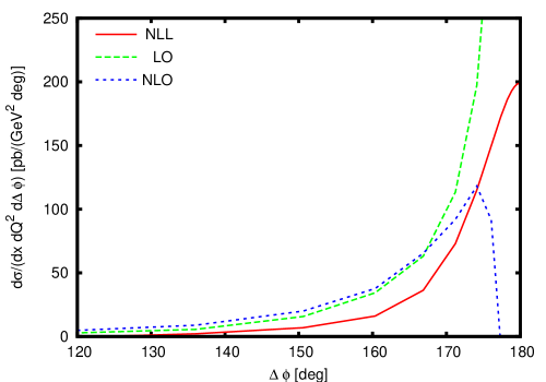
   Figure 1: The resummed $\Delta\phi$ distribution for dijets in DIS. Also shown for comparison are the leading order (LO) and next-to–leading order (NLO) predictions from NLOJET++ [7].

3. At small $b$ the radiator in eq. (11) ought to vanish for $b=0$, since this point corresponds to a complete cancelation between real and virtual correction terms. This cancelation is not present in the pure NLL approximation we obtain here. We have therefore set $R_{\mathrm{in/out}}(\bar{b})=S(\bar{b})=0$ and freezed the parton density at $\mu_{f}$ for $\bar{b}<1$. Other modifications such as the replacement $\bar{b}\to\sqrt{1+\bar{b}^{2}}$ that ensure a sensible $b=0$ behaviour can also be made but we have checked that this does not numerically alter our results presented here.

An important thing to notice is that an NLL resummation is strictly valid for $1<\bar{b}<\mu_{f}/Q_{0}$. In particular the relative size of the large-$b$ part of the integral, corresponding to $\bar{b}>\mu_{f}/Q_{0}$, can give us an idea of the impact of intrinsic parton transverse momentum, an area that we shall explore in more detail in forthcoming work [22].

We plot the resummed result for the $\Delta\phi$ distribution in fig. 1 along with the fixed-order predictions for dijet production in DIS with $Q^{2}=67$ ${\mathrm{GeV}}^{2}$ and $x_{B}=2.86\times 10^{-3}$. These values and other cuts on the jets have been taken from the H1 study [3] to which we would eventually compare our results. We fixed both renormalisation and factorisation scales to be the average transverse energy of the jets, and used CTEQ6M parton distributions [24], corresponding to $\alpha_{s}(M_{Z})=0.118$. As we can see the fixed-order predictions diverge as expected near $\Delta\phi=\pi$. This divergence is cured by the resummation that goes to a fixed non-zero value at $\Delta\phi=\pi$. Of note here is the absence of a Sudakov peak since the Sudakov mechanism does not dominate the $b$ integral at very small $\Delta=|\pi-\Delta\phi|.$ The dominant mechanism to obtain back-to–back jets is thus a one-dimensional cancelation between emissions rather than a suppression of the $k_{t}$ of each individual emission, leading to a washout of the Sudakov peak as explained in detail in ref. [15].

In order to obtain complete predictions which can be compared to data two further developments need to be made. The first concerns matching to fixed order which is non-trivial since it requires information on the flavour of all the partons in the event which is not directly available in the fixed-order codes. Here we hope to exploit recent developments in this regard [25] which have addressed these issues in the context of hadron collider event shapes [26]. Secondly non-perturbative effects are expected to play an important role in the region $\Delta\phi\approx\pi$ where they can be expected to significantly change the value of the distribution. Here one can apply a Gaussian smearing to our $b$-space results as is the practice for vector boson $Q_{t}$ spectra [27] as a model for non-perturbative effects whose parameters can be constrained phenomenologically. We leave both these developments for forthcoming work [22].

References

- [1] A. Aktas et al. [H1 Collaboration], Eur. Phys. J. C 33 (2004) 477 [arXiv: hep-ex/0310019].
- [2] S. Chekanov et al. [ZEUS Collaboration], Nucl. Phys. B 786 (2007) 152 [arXiv: 0705.1931 [hep-ex]].
- [3] M. Hansson [H1 Collaboration], Prepared for International Workshop on Deep Inelastic Scattering (DIS 2006), Tsukuba, Japan, 20-24 Apr 2006 [H1prelim-06-032].
- [4] V. M. Abazov et al. [DØ Collaboration], Phys. Rev. Lett. 94 (2005) 221801 [arXiv: hep-ex/0409040].
- [5] M. Hansson and H. Jung, In the proceedings of International Workshop on Deep-Inelastic Scattering and Related Subjects (DIS 2007), Munich, Germany, 16-20 Apr 2007 [arXiv: 0707.4276 [hep-ph]].
- [6] F. Hautmann and H. Jung, Presented at Photon 2007: International Conference on the Structure and Interactions of the Photon and the International Workshop on Photon-Photon Collisions and International Workshop on High Energy Photon Linear Colliders, Paris, France, 9-13 Jul 2007 [arXiv: 0712.0568 [hep-ph]].
- [7] Z. Nagy and Z. Trocsanyi, Phys. Rev. Lett. 87 (2001) 082001 [arXiv: hep-ph/0104315].
- [8] N. Kidonakis, G. Oderda and G. Sterman, Nucl. Phys. B 525 (1998) 299 [arXiv: hep-ph/9801268].
- [9] D. de Florian and W. Vogelsang, Phys. Rev. D 76 (2007) 074031 [arXiv: 0704.1677 [hep-ph]].
- [10] M. Dasgupta and G. P. Salam, Phys. Lett. B 512 (2001) 323 [arXiv: hep-ph/0104277].
- [11] M. Dasgupta and G. P. Salam, J. High Energy Phys. 0203 (2002) 017 [arXiv: hep-ph/0203009].
- [12] A. Banfi and M. Dasgupta, J. High Energy Phys. 0401 (2004) 027 [arXiv: hep-ph/0312108].
- [13] J. E. Huth et al., Presented at Summer Study on High Energy Physics, Research Directions for the Decade, Snowmass, CO, Jun 25 - Jul 13, 1990. Published in Snowmass Summer Study 1990:0134-136 [FERMILAB-CONF-90-249-E]
- [14] M. Hansson, Lund University PhD thesis, Aug 2007 [LUNFD6-NFFL-7226-2007].
- [15] A. Banfi, G. Marchesini and G. Smye, J. High Energy Phys. 0204 (2002) 024 [arXiv: hep-ph/0203150].
- [16] A. Banfi, G. Marchesini, Y. L. Dokshitzer and G. Zanderighi, J. High Energy Phys. 0007 (2000) 002 [arXiv: hep-ph/0004027].
- [17] S. Catani, L. Trentadue, G. Turnock and B. R. Webber, Nucl. Phys. B 407 (1993) 3.
- [18] A. Banfi, G. Marchesini, G. Smye and G. Zanderighi, J. High Energy Phys. 0111 (2001) 066 [arXiv: hep-ph/0111157].
- [19] N. Kidonakis, G. Oderda and G. Sterman, Nucl. Phys. B 531 (1998) 365 [arXiv: hep-ph/9803241].
- [20] A. Banfi and M. Dasgupta, Phys. Lett. B 628 (2005) 49 [arXiv: hep-ph/0508159].
- [21] Y. Delenda, R. Appleby, M. Dasgupta and A. Banfi, J. High Energy Phys. 0612 (2006) 044 [arXiv: hep-ph/0610242].
- [22] A. Banfi, M. Brambilla, M. Dasgupta and Y. Delenda, in preparation.
- [23] Y. L. Dokshitzer, G. Marchesini and B. R. Webber, J. High Energy Phys. 9907 (1999) 012 [arXiv: hep-ph/9905339].
- [24] J. Pumplin, D. R. Stump, J. Huston, H. L. Lai, P. Nadolsky and W. K. Tung, J. High Energy Phys. 0207 (2002) 012 [arXiv: hep-ph/0201195].
- [25] A. Banfi, G. P. Salam and G. Zanderighi, Eur. Phys. J. C 47 (2006) 113 [arXiv: hep-ph/0601139].
- [26] A. Banfi, G. P. Salam and G. Zanderighi, J. High Energy Phys. 0408 (2004) 062 [arXiv: hep-ph/0407287].
- [27] C. Balazs and C. P. Yuan, Phys. Rev. D 56 (1997) 5558 [arXiv: hep-ph/9704258].