Dynamical evolution of correlated spontaneous emission of a single photon from a uniformly excited cloud of N atoms

Abstract

We study the correlated spontaneous emission from a dense spherical cloud of $N$ atoms uniformly excited by absorption of a single photon. We find that the decay of such a state depends on the relation between an effective Rabi frequency $\Omega\propto\sqrt{N}$ and the time of photon flight through the cloud $R/c$. If $\Omega R/c<1$ the state exponentially decays with rate $\Omega^{2}R/c$ and the state life time is greater then $R/c$. In the opposite limit $\Omega R/c\gg 1$, the coupled atom-radiation system oscillates between the collective Dicke state (with no-photons) and the atomic ground state (with one photon) with frequency $\Omega$ while decaying at a rate $c/R$.

The problem of a single photon absorbed by a cloud of $N$ atoms followed by correlated spontaneous emission is a problem of long standing interest. Dicke Dick54 first noted that the radiation rate from a small dense cloud is abnormal. In his words “… the greatest radiation intensity anomaly occurs in the transition to the ground state” Dicke64 . In particular he showed that the collective decay rate for the symmetric state with one excitation is $\Gamma_{N}=N\gamma$ (as indicated in Fig. 1(a)), where he assumed the atomic volume to have dimensions small compared with the radiation wavelength.

In our present work, we are interested in the time evolution of a specially prepared state obtained by absorption of a single photon Scul06a ; Scul06b ; kurizki . We report novel dynamical oscillations in the evolution of the quantum state of the atom cloud, even without the existence of a cavity. Fig. 1 summarizes the main results of this paper. It is as if the atomic cloud acts to form a new “cavity” with the atom cloud volume $V$ replacing the virtual photon volume $\mathcal{V}_{\text{ph}}$ defined by the electromagnetic cavity; that is the usual vacuum Rabi frequency $\Omega_{\text{Vac}}=(\wp/\hbar)\sqrt{\hbar\omega/(\epsilon_{0}\mathcal{V}_{\text{ph}})}$ is replaced by $\Omega_{0}=(\wp/\hbar)\sqrt{\hbar\omega/(\epsilon_{0}V)}$ in the present problem, where $\wp$ is the electric-dipole transition matrix element, $\hbar\omega$ is the photon energy and $\epsilon_{0}$ is free space permittivity.

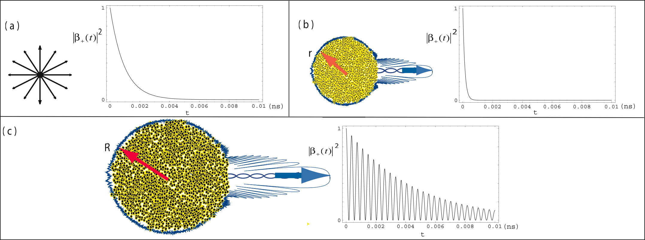
Figure 1: Comparison of the different dynamical behavior for the correlated spontaneous emission from an $N$ atomic cloud described by the $|+\rangle_{{\mathbf{k}}_{0}}$ state of Fig. 2b. The single atom spontaneous decay life time is taken to be $\tau_{0}=10$ ns ($\gamma=1/2\tau_{0}$). We assume that atomic density is $10^{16}$cm^-3 and the resonant photon wavelength is $\lambda=1\mu$m. Plot (a) corresponds to the case when cloud radius is equal to $\lambda/2$, hence the number of atoms is $N_{a}=5240$, then the state decay time is $\tau_{a}=\tau_{0}/N_{a}=1.9\times 10^{-3}$ ns. In plot (b) the cloud radius is $r=10\lambda$, $N_{b}=4.2\times 10^{7}$, $\tau_{b}=32\pi^{2}r^{2}\tau_{0}/27N_{b}\lambda^{2}=2.7\times 10^{-4}$ ns. In plot (c) the radius of the atomic cloud is $R=1$ mm which yields $N_{c}=4.1\times 10^{13}$, $\tau_{c}=8R/6c=4.4\times 10^{-3}$ ns, while the period of oscillations is $2\pi/\Omega=0.74\times 10^{-3}$ ns.

Here we analytically solve the equation of motion for the system in two regimes. In one regime, we find that, for finite atom cloud size, the atomic excitation will decay with a rate determined by the photon escape time, together with fast dynamical oscillations (as indicated in Fig. 1(c)) with the effective Rabi oscillation frequency $\Omega$ proportional to $\sqrt{N}$.

However, if the oscillation period is much greater then the time of photon flight through the cloud, the atomic state will decay exponentially. For a small cloud ($R\ll\lambda$) the decay rate is $N\gamma$, where $\gamma$ is the single atom decay rate, see Fig. 1a. For a larger cloud ($R\gg\lambda$ but $\Omega R/c\ll 1$) the decay rate goes as $N\gamma(\lambda/R)^{2}$ as in Fig. 1b. Finally, for an even larger cloud ($\Omega R/c\gg 1$) the probability of photon emission oscillates while decaying with a rate $\sim c/R$, see Fig. 1c.

These two regimes (b and c) are determined by whether the system persists memory effect, i.e., non-Markovian or Markovian regimes. We discuss connection with previous work elberly2006 ; Cumm86 ; benivegna ; buzek ; buzek2 ; eberly at the end of this paper.

We consider a system of N two-level ($a$ excited and $b$ ground) atoms, initially one of them is in the excited state $a$ (with no information which one), $E_{a}-E_{b}=\hslash\omega$, and the multi-mode radiation field is in the vacuum. Atoms are located at positions $\mathbf{r}_{j}$ ($j=1,...,N$). The whole set of states can be expressed as those in Fig. 2 Scul06b , where $|j\rangle\,\,\,=|b_{1},b_{2},...,b_{j-1},a_{j},b_{j+1}...b_{N}\rangle$ represents the state in which the $j^{th}$ atom is exited but the others are in the ground state and $|g\rangle=|b_{1},b_{2},...,b_{N}\rangle$ is the state with all the atoms in the ground state. The atomic state prepared by uniformly absorbing one single photon with wavevector $\mathbf{k}_{0}$ is exactly the $|+\rangle_{\mathbf{k}_{0}}$ state of Fig. 2b. In the limit $R\gg\lambda$ we focus here the $|+\rangle_{\mathbf{k}_{0}}$ state is approximately an eigenstate of the system Scul06b . This makes the basis set of Fig. 2b preferable. The state vector for the atom-field system at time $t$ can be then written as

$$|\Psi(t)\rangle=[\beta_{+}(t)|+\rangle_{\mathbf{k}_{0}}+\beta_{1}(t)|1\rangle_{\mathbf{k}_{0}}+\beta_{2}(t)|2\rangle_{\mathbf{k}_{0}}+...$$

$$+\beta_{N-1}(t)|N-1\rangle_{\mathbf{k}_{0}}]|0\rangle+\sum_{\mathbf{k}}\gamma_{\mathbf{k}}(t)|g\rangle|1_{\mathbf{k}}\rangle\,,$$ (1)

with initial conditions $\beta_{+}(0)=1$ and all other probability amplitudes are zero. In the dipole approximation the atom-field interaction is described by the Hamiltonian

$$\hat{H}_{\text{int}}=\sum_{\mathbf{k}}\sum_{j=1}^{N}\hbar g_{k}\left[\hat{\sigma}_{j}\hat{a}_{\mathbf{k}}^{{\dagger}}\exp(i(\omega_{k}-\omega)t-i\mathbf{k\cdot r}_{j})+\text{adj}\right],$$ (2)

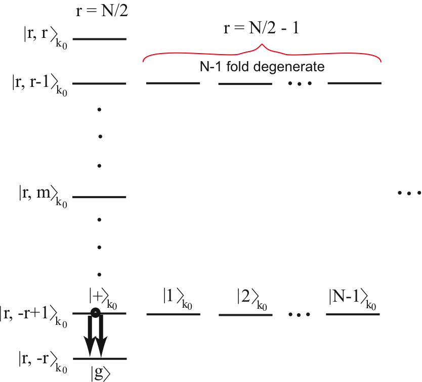
(a) $\displaystyle|+\rangle_{{\mathbf{k}}_{0}}$ $\displaystyle=$ $\displaystyle\frac{1}{\sqrt{N}}\sum_{j}e^{i{\mathbf{k}}_{0}\cdot{\mathbf{r}}_{j}}|j\rangle$ $\displaystyle|1\rangle_{{\mathbf{k}}_{0}}$ $\displaystyle=$ $\displaystyle\frac{1}{\sqrt{2}}\left[|1\rangle e^{i{\mathbf{k}}_{0}\cdot{\mathbf{r}}_{1}}-|2\rangle e^{i{\mathbf{k}}_{0}\cdot{\mathbf{r}}_{2}}\right]$ $\displaystyle|2\rangle_{{\mathbf{k}}_{0}}$ $\displaystyle=$ $\displaystyle\frac{1}{\sqrt{6}}\left[|1\rangle e^{i{\mathbf{k}}_{0}\cdot{\mathbf{r}}_{1}}+|2\rangle e^{i{\mathbf{k}}_{0}\cdot{\mathbf{r}}_{2}}-2|3\rangle e^{i{\mathbf{k}}_{0}\cdot{\mathbf{r}}_{3}}\right]$ $\displaystyle\cdot$ $\displaystyle\cdot$ $\displaystyle\cdot$ $\displaystyle|N-1\rangle_{{\mathbf{k}}_{0}}$ $\displaystyle=$ $\displaystyle\frac{1}{\sqrt{(N-1)N}}[|1\rangle e^{i{\mathbf{k}}_{0}\cdot{\mathbf{r}}_{1}}+|2\rangle e^{i{\mathbf{k}}_{0}\cdot{\mathbf{r}}_{2}}+\cdot\cdot\cdot$ $\displaystyle+|N-1\rangle e^{i{\mathbf{k}}_{0}\cdot{\mathbf{r}}_{N-1}}-(N-1)|N\rangle e^{i{\mathbf{k}}_{0}\cdot{\mathbf{r}}_{N}}]$ (b)

Figure 2: Timed Dicke states associated with absorption of radiation of wave vector ${\mathbf{k}}_{0}$: (a) the initial state $|+\rangle_{\mathbf{k}_{0}}$ decays directly to the graund state $|g\rangle$. (b) the timed Dicke states corresponding to single photon excitations.

where $\hat{\sigma}_{j}$ is the lowering operator for atom $j$, $\hat{a}_{\mathbf{k}}$ is the photon operator and $g_{k}=\wp\sqrt{\hbar\omega_{k}/(\epsilon_{0}\mathcal{V}_{\text{ph}})}$ is the atom-photon coupling constant for the ${\mathbf{k}}$ mode, $\omega_{k}$ is the photon frequency and $\omega=ck_{0}$ is the energy difference between level $a$ and $b$, $c$ is the speed of light. For simplicity, we neglect the effects of photon polarization. The dynamical evolution is then totally determined by the Schrödinger’s equation. Let us consider first the two atoms problem, and call the state $|1\rangle_{\mathbf{k}_{0}}=|-\rangle_{\mathbf{k}_{0}}$. The state vector for the two atoms plus field system is then given by

$$|\Psi(t)\rangle=\beta_{+}(t)|+\rangle_{{\mathbf{k}}_{0}}|0\rangle+\beta_{-}(t)|-\rangle_{{\mathbf{k}}_{0}}|0\rangle+\sum_{{\mathbf{k}}}\gamma_{{\mathbf{k}}}(t)|g\rangle|1_{{\mathbf{k}}}\rangle.$$ (3)

As is shown in Ref. Scul06b , the probability amplitude $\beta_{+}$ and $\beta_{-}$ are coupled due to the fact that they decay to a common ground state, that is

$$\dot{\beta}_{+}=-\gamma_{++}\beta_{+}-\gamma_{+-}\beta_{-},$$ (4)

$$\dot{\beta}_{-}=-\gamma_{--}\beta_{-}-\gamma_{-+}\beta_{+}.$$ (5)

This was first pointed out by Agarwal agarwal . It is closely related to earlier work of Fano, and is often referred to as Fano coupling. We call it Agarwal-Fano coupling.

However, when we consider a sphere with $N$ atoms, where $N\gg 1$, and $R\gg\lambda$ there is no Agarwal-Fano coupling. Instead we now find Scul06b

$$\dot{\beta}_{+}(t)=-\frac{1}{N}\int_{0}^{t}dt^{\prime}\sum_{{\mathbf{k}}}\sum_{i,j=1}^{N}g_{k}^{2}\exp[i(\omega_{k}-\omega)(t^{\prime}-t)]$$

$$\cdot\exp[i({\mathbf{k}}-{\mathbf{k}}_{0})\cdot({\mathbf{r}}_{i}-{\mathbf{r}}_{j})]\beta_{+}(t^{\prime}).$$ (6)

For a dense cloud one can treat the atom distribution as continuous, we then have $\sum_{i,j}\rightarrow\left(N/V\right)^{2}\int d{\mathbf{r}}\int d{\mathbf{r}}^{\prime}$, where $V=4\pi R^{3}/3$ is the volume of the spherical atomic cloud. The summation over ${\mathbf{k}}$ can also be replaced by integration $\sum_{{\mathbf{k}}}\rightarrow\displaystyle\mathcal{V}_{\text{p}h}/(2\pi)^{3}\int d{\mathbf{k}},$ where $\mathcal{V}_{\text{ph}}$ is the photon volume. Then the equation of motion reads

$$\dot{\beta}_{+}(t)=-\frac{\mathcal{V}_{\text{ph}}}{(2\pi)^{3}}\frac{N}{V^{2}}\int d\mathbf{k}\int d\mathbf{r}\int d\mathbf{r}^{\prime}g_{k}^{2}\int_{0}^{t}dt^{\prime}\beta_{+}(t^{\prime})$$

$$\cdot\exp[i(\omega_{k}-\omega)(t^{\prime}-t)+i(\mathbf{k}-\mathbf{k}_{0})\cdot(\mathbf{r}-\mathbf{r}^{\prime})]\,.$$ (7)

In the limit $R\rightarrow\infty$ integration over $\mathbf{r}^{\prime}$ gives the delta-function

$$\int d\mathbf{r}^{\prime}\exp[-i(\mathbf{k-k}_{0})\mathbf{r}^{\prime}]=(2\pi)^{3}\delta(\mathbf{k-k}_{0}),$$

and thus we obtain

$$\dot{\beta}_{+}(t)=-N\Omega_{0}^{2}\int_{0}^{t}dt^{\prime}\beta_{+}(t^{\prime})\,,$$ (8)

where we have defined $\Omega_{0}=(\wp/\hbar)\sqrt{\hbar\omega/(\epsilon_{0}V)}$, which is like vacuum Rabi frequency but with atomic volume $V$ replacing photon volume $\mathcal{V}_{\text{ph}}$.

Differentiating both sides of Eq. (8) yields a harmonic oscillator equation

$$\ddot{\beta}_{+}(t)+\Omega^{2}\beta_{+}(t)=0,$$ (9)

where $\Omega=\sqrt{N}\Omega_{0}$ is an effective Rabi frequency. Therefore in the limit $R\rightarrow\infty$ the atomic state undergoes harmonic oscillations with the effective Rabi frequency $\Omega$

$$\beta_{+}(t)=\cos(\Omega t).$$ (10)

To find a solution of Eq. (7) at finite $R$, but yet $k_{0}R\gg 1$, we rewrite it as

$$\dot{\beta}_{+}(t)=-\frac{2\mathcal{V}_{\text{ph}}N}{\pi V^{2}}\int d\mathbf{k}g_{k}^{2}\int_{0}^{t}dt^{\prime}\beta_{+}(t^{\prime})e^{i(\omega_{k}-\omega)(t^{\prime}-t)}S({\mathbf{k},R})^{2},$$ (11)

where

$$S({\mathbf{k},R})=\frac{1}{4\pi}\int_{V}d\mathbf{r}\exp[i(\mathbf{k-k}_{0})\mathbf{r}]$$

$$=\frac{\sin(|\mathbf{k-k}_{0}|R)}{|\mathbf{k-k}_{0}|^{3}}-\frac{R\cos(|\mathbf{k-k}_{0}|R)}{|\mathbf{k-k}_{0}|^{2}}.$$ (12)

Next we approximate $g_{k}^{2}\approx g_{k_{0}}^{2}$ and replace integration over $\mathbf{k}$ by integration over $\mathbf{p}=\mathbf{k-k}_{0}$. The main contribution to the integral comes from the region $p\lesssim 1/R$. That is under the exponent one can replace $k-k_{0}\simeq\mathbf{k}_{0}\cdot\mathbf{p}/k_{0}$. Then Eq. (11) reads

$$\dot{\beta}_{+}(t)=-\frac{2}{\pi}N\Omega_{0}^{2}\int d\mathbf{p}\int_{0}^{t}dt^{\prime}\beta_{+}(t^{\prime})e^{[ic\mathbf{k}_{0}\cdot\mathbf{p}(t^{\prime}-t)/k_{0}]}$$

$$\left[\frac{\sin(pR)}{p^{3}}-\frac{R\cos(pR)}{p^{2}}\right]^{2}.$$ (13)

Integration over directions of $\mathbf{p}$ yields

$$\dot{\beta}_{+}(t)=-\frac{8}{c}N\Omega_{0}^{2}\int_{0}^{\infty}pdp\int_{0}^{t}dt^{\prime}\beta_{+}(t^{\prime})$$

$$\cdot\frac{\sin[cp(t^{\prime}-t)]}{(t^{\prime}-t)}\left[\frac{\sin(pR)}{p^{3}}-\frac{R\cos(pR)}{p^{2}}\right]^{2}.$$ (14)

To integrate over $p$ we use the following formula

$$\int_{0}^{\infty}pdp\frac{\sin[cp(t^{\prime}-t)]}{(t^{\prime}-t)}\left[\frac{\sin(pR)}{p^{3}}-\frac{R\cos(pR)}{p^{2}}\right]^{2}=$$

$$\left\{\begin{array}[]{c}\frac{\pi c}{96}\left[16R^{3}+12cR^{2}(t^{\prime}-t)-c^{3}(t^{\prime}-t)^{3}\right],\quad c|t^{\prime}-t|<2R\\ 0,\quad\text{otherwise}\end{array}\right.$$ (15)

which gives

$$\dot{\beta}_{+}(t)=-\frac{1}{4}N\Omega_{0}^{2}\int_{0}^{t}dt^{\prime}\beta_{+}(t^{\prime})\left[16+12\frac{c}{R}(t^{\prime}-t)\right.$$

$$\left.-\frac{c^{3}}{R^{3}}(t^{\prime}-t)^{3}\right]\Theta\left[c(t^{\prime}-t)+2R\right].$$ (16)

Next we note that the function $16+12\frac{c}{R}(t^{\prime}-t)-\frac{c^{3}}{R^{3}}(t^{\prime}-t)^{3}$ and its derivative over $t^{\prime}$ is equal to zero when $c(t^{\prime}-t)+2R=0$. Taking derivative of both sides of Eq. (16) twice we obtain:

$$\dddot{\beta}_{+}(t)=-N\Omega_{0}^{2}\left\{\dot{\beta}_{+}(t)-\frac{3c}{4R}\beta_{+}(t)\right.-$$

$$\left.\frac{3c^{3}}{8R^{3}}\int_{0}^{t}dt^{\prime}\beta(t^{\prime})(t^{\prime}-t)\Theta\left[c(t^{\prime}-t)+2R\right]\right\}.$$ (17)

Next we assume that

$$N\Omega_{0}^{2}\frac{R^{2}}{c^{2}}\gg 1,\quad\text{or}\quad\frac{\Omega R}{c}\gg 1.$$ (18)

Then one can omit the last term in Eq. (17) which yields

$$\dddot{\beta}_{+}(t)+\Omega^{2}\dot{\beta}_{+}(t)-\frac{3c\Omega^{2}}{4R}\beta_{+}(t)=0.$$ (19)

Solution of Eq. (19) under the condition (18) is given by

$$\beta_{+}(t)=\cos(\Omega t)\exp\left(-\frac{3c}{8R}t\right),$$ (20)

which describes rapid oscillations with the effective Rabi frequency $\Omega$ superimposed by the exponential decay. The state decays during the time of the photon flight through the atomic cloud. The emitted photon is reabsorbed and reemitted many times before it leaves the cloud.

In the opposite limit, $\Omega R/c\ll 1$, one can use the Markovian approximation. We integrate Eq. (16) over $t^{\prime}$ assuming $\beta_{+}(t^{\prime})$ is a slow varying function of $t^{\prime}$ and approximate $\beta_{+}(t^{\prime})\approx\beta_{+}(t)$. Then for $t>2R/c$ we obtain

$$\dot{\beta}_{+}(t)=-\Gamma\beta_{+}(t),$$ (21)

which yields an exponentially decaying solution

$$\beta_{+}(t)=\beta_{+}(0)e^{-\Gamma t}.$$ (22)

Here $\Gamma=3\Omega^{2}R/4c=27N\gamma/8(k_{0}R)^{2}$ and $\gamma=(\omega^{3}\wp^{2})/(6\pi\epsilon_{0}\hbar c^{3})$ is the spontaneous decay rate for one atom.

Discussion: Similar problems have been investigated in the past several decades. Cummings Cumm86 considered the spontaneous emission of a single atom which is initially excited in the presence of $N-1$ initially unexcited identical atoms, when there are $M$ accessible radiation modes. He showed that such an extended system oscillates between the ground sate and the excited state with an effective Rabi frequency $\Omega\sim\sqrt{N}$. Such modification of the spontaneous emission of one atom in the presence of $N-1$ atoms inside a cavity has been studied since then benivegna , buzek . Buzek buzek2 studied the dynamics of an excited atom in the presence of $N-1$ unexcited atoms in the free space and predicted that there is a radiation suppression but did not report dynamical oscillations.

The effective Rabi frequency $\Omega=\sqrt{N}\Omega_{0}$ we found from quantum mechanical consideration can be written as $\Omega=\sqrt{(3/4\pi^{2})\gamma\omega(N/V)\lambda^{3}}=\sqrt{n\omega\wp^{2}/\epsilon_{0}\hbar}$. This result is analogous to the plasma frequency and can be obtained in a classical model by treating atoms as classical harmonic oscillators burnham . Indeed, replacing the electric-dipole transition matrix element by $\wp=e\cdot d$, where $d=\sqrt{\hslash/m\omega}$ is the oscillator length, yields precisely the plasma frequency $\Omega=\sqrt{ne^{2}/m\epsilon_{0}}$.

Relevant experiments have been carried out by the groups of Lukin lukin , Kuzmich kuzmich , Kimble kimble , Vuleti$\acute{\text{c}}$ vuletic , Harris Bali05 et al. note . For realistic physical situations such as $n=10^{14}$cm^-3, $\omega/2\pi=6\times 10^{14}$Hz, $R=10$ cm ($N=4\times 10^{17}$) and $|\wp|=10^{-29}$C$\cdot$m, we obtain that the state decay is accompanied by a few oscillations with the effective Rabi frequency $\Omega\approx 2\times 10^{10}$Hz and the decay time is about $R/c\sim 3\times 10^{-10}$s. One can observe a crossover to the exponentially decaying regime, e.g., by decreasing the size of the atomic cloud.

In summary, we study correlated spontaneous emission of a totally symmetric $N$-atom state prepared by an absorption of a single photon. This is an extension of the result obtained in Refs. Scul06a ; Scul06b . Decay of such a state occurs via photon emission in the direction of the incident photon for large enough density. We found that time evolution of the initial state depends on the relation between an effective Rabi frequency $\Omega\propto\sqrt{N}g_{k_{0}}$ and the time of photon flight through the cloud $R/c$. If $\Omega R/c<1$ the state exponentially decays with the rate $\Omega^{2}R/c$ which is determined by the Dicke superradiance rate $N\gamma$ reduced by the factor of $\lambda^{2}/R^{2}$ due to smaller finite state phase volume in the case of directional emission. In the opposite limit $\Omega R/c\gg 1$ the decay is accompanied by oscillations with the effective Rabi frequency $\Omega$ and the decay time is given by $R/c$.

We gratefully acknowledge the support of the Office of Naval Research (Award No. N00014-03-1-0385) and the Robert A. Welch Foundation (Grant No. A-1261).

References

(1) R.H. Dicke, Phys. Rev. 93, 99 (1954).
(2) R. H. Dicke, Quantum Electronics, proceedings of the third
international congress, Columbia University Press, New York (1964).
(3) M. Scully, E. Fry, C.H.R. Ooi and K. Wodkiewicz, Phys.
Rev. Lett. 96, 010501 (2006).
(4) M. Scully, Laser Phys. 17, 635 (2007) .
(5) I. E. Mazets and G. Kurizki, J. Phy. B: At. Mol. Opt.
Phys. 40, F105 (2007).
(6) J. H. Eberly, J. Phys. B: At. Mol. Opt. Phys. 39, S599 (2006).
(7) F.W. Cummings, Phys. Rev. A 33, 1683 (1986); F.W.
Cummings, Phys. Rev. Lett. 54, 2329 (1985); F.W. Cummings and A.
Dorri, Phys. Rev. A 28, 2282 (1983).
(8) G. Benivegna ad A. Messina, Phys. Lett. A 126,
249 (1988).
(9) V. Buzek, G. Drobny, M. G. Kim, M. Havukainen, and P. L.
Knight, Phys. Rev. A 60, 582 (1999).
(10) V. Buzek, Phys. Rev. A 39, 2232 (1989).
(11) N. E. Rehler and J. H. Eberly, Phys. Rev. A 3,
1735 (1971).
(12) G. Agarwal, “Quantum Statistical Theories of Spontaneous
Emission” in Springer Tracts in Modern Physics, vol. 70 (Springer-Verlag:
Berlin, 1976).
(13) D. C. Burnham and R. Y. Chiao, Phys. Rev. 188,
667 (1969).
(14) C.H. van der Wal, M.D. Eisaman, A. Andre, R.L. Walsworth,
D.F. Philips, A.S. Zibrov and M.D. Lukin, Science 301, 196 (2003).
(15) T. Chanelire, D. N. Matsukevich, S. D. Jenkins, S.-Y. Lan,
T. A. B. Kennedy and A. Kuzmich, Nature 438, 833 (2005).
(16) C.W. Chou, J. Laurat, H. Deng, K.S. Choi, H. de Riedmatten,
D. Felinto, H.J. Kimble, Science 316, 1316 (2007).
(17) A. T. Black, J. K. Thompson, and V. Vuleti, Phys. Rev. Lett. 95, 133601 (2005).
(18) V. Balic, D. A. Braje, P. Kolchin, G.Y. Yin, and S. E.
Harris, Phys. Rev. Lett. 94, 183601 (2005).
(19) To put the present results in context we emphasize the
difference between the physics of the groups of Kimble, Harris and Lukin and
the present work. In their experiment the Rabi oscillations in the two
photon correlation function are governed by the probe laser strength and
decay with the atomic decay rate. In the present work and the state decays with a rate determined by the time of photon flight
across the atomic cloud.
(a)
(b)
(a)
(b)