Bistability and mode interaction in microlasers

Abstract

We investigate the possibility of bistable lasing in microcavity lasers as opposed to bulk lasers. To that end, the dynamic behavior of a microlaser featuring two coupled, interacting modes is analytically investigated within the framework of a semiclassical laser model, suitable for a wide range of cavity shapes and mode geometries. Closed-form coupled mode equations are obtained for all classes of laser dynamics. We show that bistable operation is possible in all of these classes. In the simplest case (class-A lasers) bistability is shown to result from an interplay between coherent (population-pulsation) and incoherent (hole-burning) processes of mode interaction. We find that microcavities offer better conditions to achieve bistable lasing than bulk cavities, especially if the modes are not degenerate in frequency. This results from better matching of the spatial intensity distribution of microcavity modes. In more complicated laser models (class-B and class-C) bistability is shown to persist for modes even further apart in frequency than in the class-A case. The predictions of the coupled mode theory have been confirmed using numerical finite-difference time-domain calculations.

I Introduction

In recent years, microlasers have been an object of growing interest in the photonics community because of a remarkable promise in both basic and applied research. Modern technology has facilitated fabrication of high-$Q$ micro- and nanosized cavities (microresonators) in a vast variety of designs (microdisks, -rings, -gears, -toroids, nanowires, nanoposts, and so on VahalaReview ). Lasers can be based on many of these set-ups as well as on different materials, e.g., semiconductors, impurity ions, or dye molecules. In addition, periodic nanostructures (photonic crystals, PhCs) can provide both cavity-based and distributed feedback resonators suitable for laser design PBGdefect ; PBGlaser . The cavity size, which becomes so small as to be comparable to the operating wavelength, is what makes a microlaser physically distinct from conventional (“bulk”) cavities whose size is far larger. The small size limits the number of cavity modes that could take part in lasing, and at the same time greatly increases the influence of the cavity shape on the character of the modes. As a result, the mode structure becomes more complicated and heavily dependent on the specific cavity design. One is no longer able to describe the modes universally in an analytical manner. The variety of laser dynamics becomes much richer, which complicates the studies of microlasers to a considerable extent but at the same time can harbor interesting new effects. For example, one could look for new possibilities of bistable or multistable lasing BabaDisks , which would prove useful in many applications such as multiple-wavelength light sources, optical flip-flop devices or optical memory cells NatRings .

In the simplest case when two modes coexist in the same laser cavity (competing for the same saturable gain medium), three lasing regimes are usually considered Siegman . First, when one of the modes has an advantage (e.g., larger $Q$-factor or better coupling to the gain), it simply dominates, becoming the only lasing mode (single mode lasing). Second, when the modes are well balanced (i.e., similar $Q$-factors and equally well coupled to the gain), they can both lase simultaneously. Such a coexistence can become possible because the modes with different frequency and/or spatial field pattern preferably interact with different gain centers. As a consequence, the spectral and spatial hole burning causes each mode to get saturated independently and allow the mode that happens to be weaker to catch up with the stronger one. Each mode saturates itself more readily as it does the other mode; in this sense, the coexisting modes are said to be weakly coupled (simultaneous multimode lasing). Third, if the reverse is true, i.e., if each mode saturates the other mode before coming to its own saturation (the modes are strongly coupled), the weaker mode is quenched by the stronger one before it has any chance to catch up. Whichever mode has an initial advantage wins the competition and becomes the only lasing mode (bistable multimode lasing). The system can lase in either mode and is in this sense bistable.

Trying to understand the physical origin of strong mode coupling brings about certain problems. It was pointed out from the beginning LambLaser that harmonic modes (such as longitudinal modes in bulk cavities) must always be coupled weakly because the antinodes of the field (the regions where the light-matter interaction is maximized) are spatially mismatched for different modes. Spatial hole burning would work similarly for any two modes with mismatched intensity distribution (such as transverse modes in bulk cavities). One of the ways to circumvent this limitation is to use degenerate modes with identical spatial intensity profiles, e.g., polarization degenerate modes or counterpropagating modes in ring lasers. This can make the lasing bistable due to additional mode coupling through population pulsations diRing ; Siegman . Alternatively, one can place a saturable absorber in addition to the saturable gain medium into the cavity mcSatAbsorb ; mcSatAbsorb2 ; LambLaser . Such an absorber can be naturally realized when only a part of the active medium is pumped. Both principles can be adapted for use in microlasers and are embodied in the form of polarization-bistable and absorptive bistable laser diodes diPBLD . It has also been shown that two coupled lasers can achieve bistability if the output from each laser is directed to the other one and the feedback is reduced to prevent formation of a compound cavity mcCoupledAgrawal ; mcCoupledOudar . Later studies mcWieczorekOC ; mcWieczorekPRA give a detailed account on the stability and mode locking regimes of bulk coupled lasers based on nonlinear bifurcation analysis of the corresponding rate equations. It is fundamentally problematic to achieve similar behavior in microlasers where the modes share the same cavity. Recent achievements in the design of bistable multimode-interference laser diodes diMMI-BLD , though capable of bistable lasing within a cavity of sub-millimeter size, still require saturable absorbers for the device to function properly.

In the meantime, recent results show that there are yet unexplored possibilities for bistable operation of microlasers. We have shown zhukPRL that a cavity based on coupled defects in a PhC exhibits bistability without the need for saturable absorption or similar additional mechanisms. The same idea was seen to work in lasers based on multimode nanopillar waveguides zhukPSS . Similar results have been reported based on coupled microdisk BabaDisks and coupled microring NatRings resonators, the latter proposed for an ultrafast, ultralow-power optical memory cell design. Also, Ref. diRingFlipFlop reports that coupled multiple-feedback ring lasers can be brought to bistability by carefully selecting the feedback times, which may be more feasible in microlasers than the conventional gain-quenching scheme as in mcCoupledOudar . Finally, a time-independent multimode laser theory recently developed by H. Türeci and co-workers Tureci06 ; Tureci07 reports that mode interaction can be very important in highly multimode nanostructure-based systems such as random lasers TureciScience . In view of this, there is a pronounced need to address the question of bistability in microresonators with their specific features such as complex cavity shapes and mathematically complex cavity modes taken into account consistently. Spatial hole burning should also be accounted for rigorously without reverting to averaging approximations, which are usually applied for coupled or semiconductor lasers BabaDisks ; mcCoupledAgrawal ; mcWieczorekPRA .

In this paper, we consider the dynamics of two interacting modes in a microresonator-based laser. The semiclassical rate-equation model based on the Maxwell-Bloch equations is used to model a laser-active medium. Coupled mode equations are derived and analyzed for different classes of laser dynamics. Compared to existing accounts on mode dynamics and coupled lasers mcHodges ; mcWieczorekOC ; mcWieczorekPRA ; mcJohnBusch , no specific form is assumed for either the cavity or the mode geometry. The spatial distribution of population inversion is taken into account fully in terms of projections onto the modes’ subspace (see zhukFDTD ) for all classes of laser dynamics. The theory developed here can be seen as complementary to the account in Refs. Tureci06 ; Tureci07 by being able to provide a description of time-dependent laser dynamics. Though they are rather different, both these approaches go beyond the third-order nonlinearity in the description of light-matter interaction.

In the simplest case of class-A laser dynamics, the equations suitable for analytical studies have been derived. As already shown earlier for some particular cases (see, e.g., mcWieczorekPRA ), we confirm that coherent mode interaction (population pulsations) can result in bistable laser operation. We show that bistable lasing becomes increasingly more difficult to achieve as the intermode frequency spacing $\Delta\omega$ increases from zero. However, for microcavity modes with well-matched intensity-gain overlap the bistability window has been shown to be much greater (by up to several orders of magnitude with respect to $\Delta\omega$) than for harmonic bulk-cavity modes. A non-symmetric system, where one of the modes is given an advantage through cavity design, is also investigated. We show that a parameter mismatch favoring one of the modes can be compensated for by an opposing mismatch in another parameter that would favor the other mode. In the more complicated class-B or class-C cases, numerical studies of the obtained coupled mode equations have been carried out. The effects of increasing the pumping rate and/or $\Delta\omega$ beyond the applicability limits of the class-A approximations are studied. Bistable lasing is seen to persist unless $\Delta\omega$ becomes comparable to the width of the gain line. Even then, bistability can be further restored by increasing the pumping rate highly above threshold. The results obtained for the class-B/C microlaser systems in the framework of the coupled mode theory have been compared with full numerical finite difference time domain (FDTD) calculations. At least for the system considered (coupled defects in a 2D photonic crystal as in Ref. zhukPRL ), we demonstrate that the predictions of the theory are in a good agreement with the results of numerical simulations.

The paper is structured as follows. In Section II, we derive the semiclassical coupled two-mode laser equations suitable for a wide range of microcavity modes. Only a few general assumptions about the cavity shape are made and no particular form for the mode geometry is specified. The derivation starts from the Maxwell-Bloch equations and is carried out from the more general (class-C) through the intermediate (class-B) to the most restrictive (class-A) laser dynamics. Specific issues pertaining to introducing the dynamics classes in multimode lasers are addressed along the way. The analysis of the equations obtained is then carried out in the reverse order. In Section III, we analyze the class-A case, which, with some assumptions, turns out to be closely related to the standard two-mode competition model Siegman . The parameter window of bistable operation is investigated in terms of the spatial and spectral mode properties. In Section IV, class-B and class-C equations are numerically investigated, and the main differences with the class-A model as regards bistable lasing operation are discussed. Finally, Section V summarizes the paper.

II Coupled two-mode laser equations

II.1 Semiclassical laser equations and multimode expansion

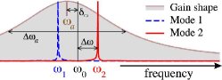
Figure 1: (Color online) Schematic illustration of the mode frequencies ($\omega_{1,2}\equiv\omega_{0}\mp\Delta\omega$) with respect to gain ($\delta_{\omega}=\omega_{a}-\omega_{0}$), as used throughout the paper.

The semiclassical laser equations used in the present paper as a starting point are composed of three parts: (i) the laser rate equations, reduced to the equation for population inversion $W$ of the laser transition; (ii) the equation of motion for the macroscopic polarization density $P$ of the laser medium, obtained in a modified electronic oscillator model, and (iii) the scalar wave equation derived from the Maxwell equations. We consider two-dimensional (2D) systems, translationally invariant in the $\hat{\mathbf{z}}$-direction, with TM light polarization, corresponding to a wide range of 2D photonic structures. In this case the electric field is $\mathbf{E}(\mathbf{r})=E_{z}(x,z)\hat{\mathbf{z}}$, allowing us to restrict ourselves to the $z$-component of the field $E(\mathbf{r},t)=E_{z}(x,y,t)$. Applying the slowly varying envelope (SVE) approximation Siegman , the Maxwell-Bloch system of equations takes the form mcHodges

$$\frac{\partial}{\partial t}W(\mathbf{r},t) = \gamma_{\parallel}\left[R-W(\mathbf{r},t)\right]+\frac{\mathrm{i}}{4\hbar}\left[E(\mathbf{r},t)P^{*}(\mathbf{r},t)-E^{*}(\mathbf{r},t)P(\mathbf{r},t)\right],$$ (1)

$$\frac{\partial}{\partial t}P(\mathbf{r},t) = -\left(\gamma_{\perp}+\mathrm{i}\delta\right)P(\mathbf{r},t)-\frac{\mathrm{i}\mu^{2}}{\hbar}W(\mathbf{r},t)E(\mathbf{r},t),$$ (2)

$$\frac{1}{\epsilon_{0}}\frac{\partial^{2}}{\partial t^{2}}\left(P(\mathbf{r},t)\mathrm{e}^{-\mathrm{i}\omega t}\right) = \left[c^{2}\nabla^{2}-\epsilon(\mathbf{r})\frac{\partial^{2}}{\partial t^{2}}-\kappa(\mathbf{r})\frac{\partial}{\partial t}\right]\left(E(\mathbf{r},t)\mathrm{e}^{-\mathrm{i}\omega t}.\right)$$ (3)

Here $W(\mathbf{r},t)$ has the meaning of population inversion, which can vary spatially as opposed to Ref. mcWieczorekPRA where it is assumed to be constant across the whole cavity. Further, $R$ is the external pumping rate, $\mu$ is the dipole matrix element of the atomic laser transition, and the polarization and population inversion decay rates are given by $\gamma_{\perp}$ and $\gamma_{\parallel}$, respectively. We consider a resonant system that features two eigenmodes with decay rates $\kappa_{1,2}$, phenomenologically accounted for by the presence of a loss term $\kappa(\mathbf{r})$ in Eq. (3). The mode frequencies are $\omega_{1,2}\equiv\omega_{0}\mp\Delta\omega$, and the central frequency $\omega_{0}$ is shifted with respect to the lasing transition frequency $\omega_{a}$ by $\delta_{\omega}=\omega_{a}-\omega_{0}$ with $\Delta\omega,\delta_{\omega}\ll\omega_{0}$, as shown in Fig. 1. We assume that the eigenmodes of the cold cavity have a spatial structure given by $u_{1,2}(\mathbf{r})$. The electric field $E(\mathbf{r},t)$ is then decomposed into the spatially dependent mode profiles $u_{1,2}(\mathbf{r})$ multiplied by time dependent SVE functions $E_{1,2}(t)$ as

$$E(\mathbf{r},t)\mathrm{e}^{-\mathrm{i}\omega_{0}t}=u_{1}(\mathbf{r})E_{1}(t)\mathrm{e}^{-\mathrm{i}\omega_{1}t}+u_{2}(\mathbf{r})E_{2}(t)\mathrm{e}^{-\mathrm{i}\omega_{2}t}$$ (4)

$$\equiv\left[u_{1}(\mathbf{r})E_{1}(t)\mathrm{e}^{\phi_{+}}+u_{2}(\mathbf{r})E_{2}(t)\mathrm{e}^{\phi_{-}}\right]\mathrm{e}^{-\mathrm{i}\omega_{0}t}.$$

Here and further, $\phi_{\pm}\equiv\pm\mathrm{i}\Delta\omega t$. Following the approach in mcHodges , we make a similar ansatz for the polarization, introducing the amplitudes $P_{1,2}(t)$ as

$$P(\mathbf{r},t)\mathrm{e}^{-\mathrm{i}\omega_{0}t}=\left[u_{1}(\mathbf{r})P_{1}(t)\mathrm{e}^{\phi_{+}}+u_{2}(\mathbf{r})P_{2}(t)\mathrm{e}^{\phi_{-}}\right]\mathrm{e}^{-\mathrm{i}\omega_{0}t}.$$ (5)

The applicability of the expansion (5) needs further justification. Eq. (5) assumes that polarization $P(\mathbf{r},t)$ and the electric field $E(\mathbf{r},t)$ have similar spatial profiles. This is strictly true only if the field intensity is small enough, e.g., if the pumping rate $R$ is not very large. Otherwise, the polarization gets influenced by the saturation terms that involve the population inversion $W(\mathbf{r},t)$, which itself cannot be spatially decomposed. These saturation terms would modify the spatial profile of $P(\mathbf{r},t)$ outside the scope of Eq. (5).

However, as Eq. (5) does not contain any explicit expansion in a series of nonlinearity orders with subsequent series truncation, the constraint on the pumping rate $R$ appears to be much weaker than what is enforced by the usual near-threshold expansion mcZehnle ; Haken ; HakenFu , which explicitly retains only third-order nonlinearities in the hole burning interaction. In the extreme (single-mode) case, where Eq. (5) implies $P(\mathbf{r},t)\propto E(\mathbf{r},t)$ and thus carries the strongest approximation, it can be shown that the coupled mode theory based on Eq. (5) leads to underestimation of the steady-state laser field intensity $E(R)$. However, the character of the dependence $E(R)$ is preserved for the values of $R$ well outside the range of applicability of the near-threshold expansion (see Tureci06 ). Moreover, the dynamical behavior of the laser is also correctly predicted by the coupled mode theory employing the expansion (5) both for one and for two modes (see our earlier work zhukFDTD for a comparison with direct numerical simulations).

That taken into account, in what follows we will use the expansion (5), remembering that the results may deviate quantitatively and may be subjest to further checking as the pumping rate goes far above threshold.

II.2 Class-C lasers

In order to derive the equations for $E_{i}(t)$ and $P_{i}(t)$, one has to eliminate all the spatial dependencies from Eqs. (1)–(3). We begin by substituting Eqs. (4) and (5) into Eq. (3), assuming that the time dependence of the field envelopes are slow enough so that $\left|\mathrm{d}E_{j}/\mathrm{d}t\right|\ll\omega_{j}\left|E_{j}\right|$. The modes $u_{j}(\mathbf{r})$ are assumed to be orthonormal solutions of the homogeneous wave equation $(c^{2}\nabla^{2}-\epsilon(\mathbf{r})\omega_{j}^{2})u_{j}(\mathbf{r})=0$, which means that their integral across the cavity is

$$\int_{C}\varepsilon(\mathbf{r})u_{i}^{*}(\mathbf{r})u_{j}(\mathbf{r})=\delta_{ij}.$$ (6)

As a result, the spatial derivatives in Eq. (3) can be eliminated. If $\epsilon(\mathbf{r})=\epsilon$ is constant throughout the cavity (the bulk-cavity case mcHodges ), the modes in Eq.  (3) decouple rigorously, and one obtains

$$\frac{\mathrm{d}}{\mathrm{d}t}E_{j}=-\frac{\kappa_{j}E_{j}}{2}+\mathrm{\frac{i}{2\epsilon_{0}\epsilon}}\omega_{j}P_{j}.$$ (7)

This decoupling remains approximately true if the major part of the modes’ energy are located in a material with the same dielectric constant, as is often the case in microcavities. For details we refer the reader to our earlier work zhukFDTD . A more complicated case of distributed feedback structures would require additional spatial multiscale analysis, e.g., following the approach developed for photonic crystal lasers mcJohnBusch .

Eliminating spatial dependencies in Eq. (2) is simpler and requires substitution of Eqs. (4)–(5) with subsequent projection onto the eigenmodes, i.e., integration $\int u_{j}^{*}(\ldots)\mathrm{d}^{3}\mathbf{r}$ over the gain medium:

$$\frac{\mathrm{d}}{\mathrm{d}t}P_{1}= -\beta_{1}P_{1}-\mathrm{i}\frac{\mu^{2}}{\hbar}\left(E_{1}W_{11}+E_{2}W_{12}\mathrm{e}^{2\phi_{-}}\right),$$ (8)

$$\frac{\mathrm{d}}{\mathrm{d}t}P_{2}= -\beta_{2}P_{2}-\mathrm{i}\frac{\mu^{2}}{\hbar}\left(E_{1}W_{21}\mathrm{e}^{2\phi_{+}}+E_{2}W_{22}\right),$$

where $\beta_{1,2}=\left(\gamma_{\perp}+\mathrm{i}\delta_{\omega}\right)\pm\mathrm{i}\Delta\omega$ and $W_{ij}$ are the projections of the population inversion $W(\mathbf{r},t)$ onto the corresponding modes

$$W_{ij}(t)\equiv\epsilon\int_{G}\mathrm{d}^{3}\mathbf{r}\,u_{i}^{*}(\mathbf{r})W(\mathbf{r},t)u_{j}(\mathbf{r})$$ (9)

Analogously, by substituting Eqs. (4)–(5) into Eq. (1) and applying $\int u_{i}^{*}(\ldots)u_{j}\mathrm{d}^{3}\mathbf{r}$, one can obtain the equations for $W_{ij}$ in the following form:

$$\frac{\mathrm{d}}{\mathrm{d}t}W_{ij}= \gamma_{\parallel}\left(R_{ij}-W_{ij}\right)$$ (10)

$$- \frac{\mathrm{i}}{4\hbar}\left[E_{1}^{*}\left(\alpha_{ij}^{11}P_{1}+\alpha_{ij}^{12}P_{2}\mathrm{e}^{2\phi_{-}}\right)+E_{2}^{*}\left(\alpha_{ij}^{21}P_{1}\mathrm{e}^{2\phi_{+}}+\alpha_{ij}^{22}P_{2}\right)\right]$$

$$+ \frac{\mathrm{i}}{4\hbar}\left[E_{1}\left(\alpha_{ij}^{11}P_{1}^{*}+\alpha_{ij}^{21}P_{2}^{*}\mathrm{e}^{2\phi_{+}}\right)+E_{2}\left(\alpha_{ij}^{12}P_{1}^{*}\mathrm{e}^{2\phi_{-}}+\alpha_{ij}^{22}P_{2}^{*}\right)\right].$$

Here, $R_{ij}$ are related to $R$ in the same way as $W_{ij}$ to $W(\mathbf{r},t)$, via Eq. (9). The coefficients $\alpha_{ij}^{mn}$ are mode overlap integrals defined as:

$$\alpha_{ij}^{mn}\equiv\epsilon\int_{G}\mathrm{d}^{3}\mathbf{r}\,u_{i}^{*}(\mathbf{r})u_{j}(\mathbf{r})u_{m}^{*}(\mathbf{r})u_{n}(\mathbf{r}).$$ (11)

The integration in Eqs. (9) and (11) is performed over the gain medium where $\epsilon(\mathbf{r})=\epsilon$ is assumed to be constant. Apart from that assumption, the shape of the gain region itself can be arbitrary and does not have to be contiguous. The mode geometry can also be arbitrary unlike in the previous reports mcHodges ; mcWieczorekOC ; mcWieczorekPRA , as the inter-mode and mode-gain overlaps are accounted for in terms of $\alpha_{ij}^{mn}$ and $W_{ij}$. Note that Eqs. (8) and (10) with the definition (9) do not involve any approximations on the field or pump intensity beside the one associated with the validity of Eq. (5) as described above. Because of this, the full population inversion $W(\mathbf{r},t)$ cannot be written explicitly in terms of $W_{ij}(t)$ and $u_{1,2}(\mathbf{r})$, in contrast to $E$ and $P$, as in Eqs. (4)–(5). Also note that the rate equations (10) for the population inversion explicitly contain oscillatory terms, which originate from the beating in the superposition of the two modes with different frequencies $\omega_{1}$ and $\omega_{2}$.

II.3 Class-B lasers

Equations (7), (8), and (10) govern the dynamics of the two spectrally close, interacting modes without any assumptions on the laser dynamics besides those needed for the SVE approximation. All these equations include a decay term with a characteristic decay rate for all the variables involved. The mode amplitudes $E_{j}$ decay with the rate $\kappa_{j}$ associated with the $Q$-factors of the modes ($Q_{j}=\omega_{j}/\kappa_{j}$). The decay of all the population inversion projections $W_{ij}$ is governed by $\gamma_{\parallel}$. Finally, the polarization amplitudes $P_{j}$ decay rates are complex, $\beta_{j}=\left(\gamma_{\perp}+\mathrm{i}\delta_{\omega}\right)\pm\mathrm{i}\Delta\omega$. This complexity directly results from the multimode character of the laser under study, and in the single-mode case $\beta_{j}=\gamma_{\perp}$.

In the most general case of laser dynamics there are no restrictions on the decay rates $\kappa_{j}$, $\gamma_{\parallel}$. $\gamma_{\perp}$ (so-called class-C lasers). In reality, however, the decay rates are governed by different physical processes and often belong to different time scales (class-B or class-A lasers, see mcWieczorekOC ), which can make the analysis of the laser equations considerably simpler.

Class-B lasers are defined by $\gamma_{\perp}\gg\gamma_{\parallel},\kappa_{j}$. In the single-mode case, it would mean that the polarization relaxes and achieves saturation so fast that the polarization can be assumed to have no own dynamics and follows $E$ and $W$ adiabatically.

In the two-mode case, where the polarization dynamics is influenced by the intermode spacing $\Delta\omega$, the introduction of the class-B approximations needs to be approached with greater care. Since the right-hand side of Eqs. (8) includes oscillatory terms on the time scale of $2\Delta\omega$, one can eliminate the polarization only if these oscillations are much slower than the exponential decay due to $\gamma_{\perp}$, i.e., $\gamma_{\perp}\gg\Delta\omega$. Note that this additional condition for class-B lasing, specific for multimode lasers, becomes especially important in microlasers where the small cavity size can place the modes much further apart from each other than in the bulk cavities.

Under these assumptions, we can now eliminate the polarization adiabatically by assuming $\mathrm{d}P_{j}/\mathrm{d}t\approx 0$. Hence, Eqs. (8) assume the form

$$P_{1}= -\mathrm{i}\frac{\mu^{2}}{\hbar}\frac{1}{\beta_{1}}\left(E_{1}W_{11}+E_{2}W_{12}\mathrm{e}^{2\phi_{-}}\right),$$ (12)

$$P_{2}= -\mathrm{i}\frac{\mu^{2}}{\hbar}\frac{1}{\beta_{2}}\left(E_{1}W_{21}\mathrm{e}^{2\phi_{+}}+E_{2}W_{22}\right),$$

which causes Eqs. (7) to be modified as

$$\frac{\mathrm{d}}{\mathrm{d}t}E_{1}= -\frac{\kappa_{1}}{2}E_{1}+\mathrm{\frac{\mu^{2}}{\hbar}\frac{\omega_{1}}{2\epsilon_{0}\epsilon}\frac{1}{\beta_{1}}}\left(E_{1}W_{11}+E_{2}W_{12}\mathrm{e}^{2\phi_{-}}\right),$$ (13)

$$\frac{\mathrm{d}}{\mathrm{d}t}E_{2}= -\frac{\kappa_{2}}{2}E_{2}+\frac{\mu^{2}}{\hbar}\frac{\omega_{2}}{2\epsilon_{0}\epsilon}\frac{1}{\beta_{2}}\left(E_{1}W_{21}\mathrm{e}^{2\phi_{+}}+E_{2}W_{22}\right).$$

Analogously, substituting Eq. (12) into Eq. (10) one may obtain the equations for $W_{ij}$. Since the population inversion $W$ is real [see Eq. (1)], it follows from Eq. (9) that $W_{ji}^{*}=W_{ij}$, and in particular, $W_{jj}^{*}=W_{jj}$. Hence,

$$\frac{\mathrm{d}}{\mathrm{d}t}W_{ij}= \gamma_{\parallel}\left(R_{ij}-W_{ij}\right)$$ (14)

$$- \frac{\mu^{2}}{4\hbar^{2}}\left|E_{1}\right|^{2}\left[\alpha_{ij}^{11}\left(\frac{1}{\beta_{1}}+\frac{1}{\beta_{1}^{*}}\right)W_{11}+\left(\frac{\alpha_{ij}^{12}}{\beta_{2}}W_{21}+\frac{\alpha_{ij}^{21}}{\beta_{2}^{*}}W_{12}\right)\right]$$

$$- \frac{\mu^{2}}{4\hbar^{2}}\left|E_{2}\right|^{2}\left[\alpha_{ij}^{22}\left(\frac{1}{\beta_{2}}+\frac{1}{\beta_{2}^{*}}\right)W_{22}+\left(\frac{\alpha_{ij}^{21}}{\beta_{1}}W_{12}+\frac{\alpha_{ij}^{12}}{\beta_{1}^{*}}W_{21}\right)\right]$$

$$- \frac{\mu^{2}}{4\hbar^{2}}E_{1}^{*}E_{2}\left[\left(\frac{\alpha_{ij}^{11}}{\beta_{1}}+\frac{\alpha_{ij}^{22}}{\beta_{2}^{*}}\right)W_{12}+\alpha_{ij}^{12}\left(\frac{1}{\beta_{2}}W_{22}+\frac{1}{\beta_{1}^{*}}W_{11}\right)\right]\mathrm{e}^{2\phi_{-}}$$

$$- \frac{\mu^{2}}{4\hbar^{2}}E_{1}E_{2}^{*}\left[\left(\frac{\alpha_{ij}^{22}}{\beta_{2}}+\frac{\alpha_{ij}^{11}}{\beta_{1}^{*}}\right)W_{21}+\alpha_{ij}^{21}\left(\frac{1}{\beta_{1}}W_{11}+\frac{1}{\beta_{2}^{*}}W_{22}\right)\right]\mathrm{e}^{2\phi_{+}}.$$

Eqs. (13)–(14) are the governing equations for two-mode class-B lasers. Further knowledge about the modes in question can allow further simplification. A good example is the case when the modes are orthogonal not only withinin the whole cavity [Eq. (6)], but also in the gain region, e.g., if most of the cavity or at least the portion of the cavity with maximum mode energy is filled with the pumped gain medium:

$$\int_{G}u_{i}^{*}(\mathbf{r})u_{j}(\mathbf{r}) = \delta_{ij}.$$ (15)

In this case the overlap integrals with one out-of-place index ($\alpha_{ij}^{ii}$, $\alpha_{ii}^{ji}$, etc.) will be negligible compared to the rest of the overlaps such as $\alpha_{jj}^{jj}$, $\alpha_{jj}^{ii}$, $\alpha_{ij}^{ij}$, or $\alpha_{ji}^{ij}$. This allows to shorten Eq. (14), which then assume different forms for symmetric $W_{jj}$ vs. anti-symmetric projections $W_{ij\neq i}$:

$$\frac{\mathrm{d}}{\mathrm{d}t}W_{jj}= \gamma_{\parallel}\left(R_{jj}-W_{jj}\right)-\frac{\mu^{2}}{4\hbar^{2}}\left[\left|E_{1}\right|^{2}\alpha_{jj}^{11}\left(\frac{1}{\beta_{1}}+\frac{1}{\beta_{1}^{*}}\right)W_{11}+\left|E_{2}\right|^{2}\alpha_{jj}^{22}\left(\frac{1}{\beta_{2}}+\frac{1}{\beta_{2}^{*}}\right)W_{22}\right]$$ (16)

$$- \frac{\mu^{2}}{4\hbar^{2}}\left[E_{1}^{*}E_{2}\mathrm{e}^{2\phi_{-}}\left(\frac{\alpha_{jj}^{11}}{\beta_{1}}+\frac{\alpha_{jj}^{22}}{\beta_{2}^{*}}\right)W_{12}+E_{1}E_{2}^{*}\mathrm{e}^{2\phi_{+}}\left(\frac{\alpha_{jj}^{11}}{\beta_{1}^{*}}+\frac{\alpha_{jj}^{22}}{\beta_{2}}\right)W_{21}\right],$$

$$\frac{\mathrm{d}}{\mathrm{d}t}W_{12}= \gamma_{\parallel}\left(R_{12}-W_{12}\right)-\frac{\mu^{2}}{4\hbar^{2}}\left[\left|E_{1}\right|^{2}\left(\frac{\alpha_{12}^{12}}{\beta_{2}}W_{21}+\frac{\alpha_{12}^{21}}{\beta_{2}^{*}}W_{12}\right)+\left|E_{2}\right|^{2}\left(\frac{\alpha_{12}^{21}}{\beta_{1}}W_{12}+\frac{\alpha_{12}^{12}}{\beta_{1}^{*}}W_{21}\right)\right]$$ (17)

$$- \frac{\mu^{2}}{4\hbar^{2}}\left[E_{1}^{*}E_{2}\mathrm{e}^{2\phi_{-}}\alpha_{12}^{12}\left(\frac{1}{\beta_{2}}W_{22}+\frac{1}{\beta_{1}^{*}}W_{11}\right)+E_{1}E_{2}^{*}\mathrm{e}^{2\phi_{+}}\alpha_{12}^{21}\left(\frac{1}{\beta_{2}^{*}}W_{22}+\frac{1}{\beta_{1}}W_{11}\right)\right].$$

where $R_{12}\ll R_{jj}$ due to the mode orthogonality and, as we remember, $W_{21}=W_{12}^{*}$. Furthermore, if the modes are intensity-matched, i.e., assumed to have nearly equal intensity distribution in the gain region so that

$$\left|u_{1}(\mathbf{r})\right|^{2}\approx\left|u_{2}(\mathbf{r})\right|^{2},\quad\mathbf{r}\in G,$$ (18)

then it follows from Eq. (9) that $W_{11}=W_{22}\equiv W_{s}$ and $W_{12}=W_{21}^{*}\equiv W_{a}$, as well as from Eq. (11) that $\alpha_{jj}^{ii}=\alpha_{ji}^{ij}\equiv\alpha$ is real, while $\alpha_{ij}^{ij}\equiv\alpha^{\prime}$ can be complex. Hence,

$$\frac{\mathrm{d}}{\mathrm{d}t}W_{s}= \gamma_{\parallel}\left(R_{s}-W_{s}\right)-\frac{\mu^{2}}{4\hbar^{2}}\alpha\left[\left|E_{1}\right|^{2}\left(\frac{1}{\beta_{1}}+\frac{1}{\beta_{1}^{*}}\right)+\left|E_{2}\right|^{2}\left(\frac{1}{\beta_{2}}+\frac{1}{\beta_{2}^{*}}\right)\right]W_{s}$$ (19)

$$- \frac{\mu^{2}}{4\hbar^{2}}\alpha\left[E_{1}^{*}E_{2}\mathrm{e}^{2\phi_{-}}\left(\frac{1}{\beta_{1}}+\frac{1}{\beta_{2}^{*}}\right)W_{a}+E_{1}E_{2}^{*}\mathrm{e}^{2\phi_{+}}\left(\frac{1}{\beta_{1}^{*}}+\frac{1}{\beta_{2}}\right)W_{a}^{*}\right],$$

$$\frac{\mathrm{d}}{\mathrm{d}t}W_{a}= -\gamma_{\parallel}W_{a}-\frac{\mu^{2}}{4\hbar^{2}}\left[E_{1}^{*}E_{2}\mathrm{e}^{2\phi_{-}}\alpha^{\prime}\left(\frac{1}{\beta_{2}}+\frac{1}{\beta_{1}^{*}}\right)+E_{1}E_{2}^{*}\mathrm{e}^{2\phi_{+}}\alpha\left(\frac{1}{\beta_{2}^{*}}+\frac{1}{\beta_{1}}\right)\right]W_{s}$$ (20)

$$- \frac{\mu^{2}}{4\hbar^{2}}\left[\left|E_{1}\right|^{2}\left(\frac{\alpha^{\prime}}{\beta_{2}}W_{a}^{*}+\frac{\alpha}{\beta_{2}^{*}}W_{a}\right)+\left|E_{2}\right|^{2}\left(\frac{\alpha}{\beta_{1}}W_{a}+\frac{\alpha^{\prime}}{\beta_{1}^{*}}W_{a}^{*}\right)\right].$$

II.4 Class-A lasers

If one further assumes that $(\gamma_{\perp}\gg)\gamma_{\parallel}\gg\kappa_{j}$ (class-A lasers), the slowest-varying quantity becomes the mode decay. The population inversion follows the mode amplitudes $E_{j}(t)$ instantaneously and can be eliminated, leaving us with only two equations for the mode amplitudes. Similar to the way we have built the class-B approximation, the derivatives in Eqs. (14) are $\mathrm{d}W_{ij}/\mathrm{d}t\approx 0$. In this case, Eqs. (16)–(17) become

$$W_{jj}= R_{jj}-\frac{\mu^{2}}{4\hbar^{2}}\frac{1}{\gamma_{\parallel}}\left[\left|E_{1}\right|^{2}\alpha_{jj}^{11}\left(\frac{1}{\beta_{1}}+\frac{1}{\beta_{1}^{*}}\right)W_{11}+\left|E_{2}\right|^{2}\alpha_{jj}^{22}\left(\frac{1}{\beta_{2}}+\frac{1}{\beta_{2}^{*}}\right)W_{22}\right]$$ (21)

$$- \frac{\mu^{2}}{4\hbar^{2}}\left[E_{1}^{*}E_{2}\mathrm{e}^{2\phi_{-}}\left(\frac{\alpha_{jj}^{11}}{\beta_{1}}+\frac{\alpha_{jj}^{22}}{\beta_{2}^{*}}\right)W_{12}+E_{1}E_{2}^{*}\mathrm{e}^{2\phi_{+}}\left(\frac{\alpha_{jj}^{11}}{\beta_{1}^{*}}+\frac{\alpha_{jj}^{22}}{\beta_{2}}\right)W_{21}\right],$$

$$W_{12}= -\frac{\mu^{2}}{4\hbar^{2}}\frac{1}{\gamma_{\parallel}}\left[\left|E_{1}\right|^{2}\left(\frac{\alpha_{12}^{12}}{\beta_{2}}W_{21}+\frac{\alpha_{12}^{21}}{\beta_{2}^{*}}W_{12}\right)+\left|E_{2}\right|^{2}\left(\frac{\alpha_{12}^{21}}{\beta_{1}}W_{12}+\frac{\alpha_{12}^{12}}{\beta_{1}^{*}}W_{21}\right)\right]$$ (22)

$$- \frac{\mu^{2}}{4\hbar^{2}}\left[E_{1}^{*}E_{2}\mathrm{e}^{2\phi_{-}}\alpha_{12}^{12}\left(\frac{1}{\beta_{2}}W_{22}+\frac{1}{\beta_{1}^{*}}W_{11}\right)+E_{1}E_{2}^{*}\mathrm{e}^{2\phi_{+}}\alpha_{12}^{21}\left(\frac{1}{\beta_{2}^{*}}W_{22}+\frac{1}{\beta_{1}}W_{11}\right)\right].$$

This is a system of linear algebraic equations that can be solved for $W_{ij}$. We are aiming for equations with simple enough structure to be treated analytically, namely, equations for $E_{j}$ with up to cubic-order non-linearity as analyzed, e.g., in Siegman . Hence, we are looking for the solutions in the form

$$W_{ij}\equiv W_{ij}^{(0)}+\sum_{m,n}W_{ij}^{(m,n)}E_{m}^{*}E_{n},$$ (23)

neglecting terms with higher powers of $E$. Truncating higher-order nonlinearity corresponds physically to the case with low field intensities, i.e., just above the lasing threshold. Hence, at this point the near-threshold expansion is introduced as understood in numerous works mcZehnle ; Haken ; HakenFu . We remark that this expansion is by far a stronger approximation than the one used in assuming the form (5) for the polarization. Hence, the class-B and class-C models described in the previous sections are valid for much stronger pumping, while the class-A description that follows is valid for pumping rates only slightly above threshold. Inserted into Eqs. (21)–(22), Eq. (23) yields

$$W_{jj}\approx R_{jj}-\frac{\mu^{2}}{4\hbar^{2}}\frac{1}{\gamma_{\parallel}}\left[\left|E_{1}\right|^{2}\alpha_{jj}^{11}\left(\frac{1}{\beta_{1}}+\frac{1}{\beta_{1}^{*}}\right)R_{11}+\left|E_{2}\right|^{2}\alpha_{jj}^{22}\left(\frac{1}{\beta_{2}}+\frac{1}{\beta_{2}^{*}}\right)R_{22}\right],$$ (24)

$$W_{12}\approx -\frac{\mu^{2}}{4\hbar^{2}}\frac{1}{\gamma_{\parallel}}\left[E_{1}^{*}E_{2}\mathrm{e}^{2\phi_{-}}\alpha_{12}^{12}\left(\frac{1}{\beta_{2}}R_{22}+\frac{1}{\beta_{1}^{*}}R_{11}\right)+E_{1}E_{2}^{*}\mathrm{e}^{2\phi_{+}}\alpha_{12}^{21}\left(\frac{1}{\beta_{2}^{*}}R_{22}+\frac{1}{\beta_{1}}R_{11}\right)\right].$$

Note that the right-hand side of Eqs. (21)–(22) has terms of the form $E_{m}^{*}E_{n}W_{ij}$. Hence the same result could be obtained by solving the equation system $W_{ij}=\mathbb{L}\cdot W_{ij}$ iteratively as $W_{ij}^{(k)}=\mathbb{L}\cdot W_{ij}^{(k-1)}$ with $W_{ij}^{(0)}=0$ up to $W_{ij}^{(2)}$, as was done in mcHodges ; mcWieczorekPRA ; zhukPRL .

Note that the presence of oscillatory exponents $\mathrm{e}^{2\phi_{\pm}}$ on the right-hand side of Eqs. (14), induced by beating of the field intensities, dictates that an adiabatic elimination can only be performed safely if $\gamma_{\parallel}\gg\Delta\omega$. Unfortunately, this assumption is quite restrictive and makes the resulting class-A laser equations hardly applicable for any two-mode system beyond the case of spectrally overlapping modes unless the mode $Q$-factors become very high. However, Eq. (24) suggests that $W_{12}$ should be oscillatory with frequency $2\Delta\omega$. This is indeed the case, as confirmed by numerical solution of class-B or class-C equations. These oscillations (also called population pulsations) are the main reason why the condition $\mathrm{d}W_{12}/\mathrm{d}t\approx 0$ is valid only for vanishingly small $\Delta\omega$. By accounting for these pulsations explicitly, one can build class-A laser equations applicable for a wider range of $\Delta\omega$. We introduce oscillatory terms $\mathrm{e}^{\pm 2\mathrm{i}\Delta\omega t}$ into $W_{12}$:

$$W_{12}(t)=W_{21}(t)=\tilde{W}_{a}(t)\mathrm{e}^{2\phi_{+}}+\tilde{W}_{a}^{*}(t)\mathrm{e}^{2\phi_{-}}$$ (25)

where the envelope function $\tilde{W}_{a}(t)$ supposedly varies more slowly than $2\Delta\omega$ and on the same time scale as $W_{jj}(t)$. We can then reformulate the condition for adiabatic elimination of $W_{12}$ in the form $\mathrm{d}\tilde{W}_{a}/\mathrm{d}t\approx 0$. The algebraic equation for $\tilde{W}_{a}$ analogous to (22) is then

$$\tilde{W}_{a}= -\frac{\mu^{2}}{4\hbar^{2}}\frac{1}{\gamma_{\parallel}+2\mathrm{i}\Delta\omega}\left[\left|E_{1}\right|^{2}\left(\frac{\alpha_{12}^{12}}{\beta_{2}}+\frac{\alpha_{12}^{21}}{\beta_{2}^{*}}\right)\tilde{W}_{a}+\left|E_{2}\right|^{2}\left(\frac{\alpha_{12}^{21}}{\beta_{1}}+\frac{\alpha_{12}^{12}}{\beta_{1}^{*}}\right)\tilde{W}_{a}+E_{1}E_{2}^{*}\alpha_{12}^{21}\left(\frac{1}{\beta_{2}^{*}}W_{22}+\frac{1}{\beta_{1}}W_{11}\right)\right],$$ (26)

Note that unlike $W_{12}$, $\tilde{W}_{a}$ is explicitly complex due to the substitution $\gamma_{\parallel}\to\gamma_{\parallel}+2\mathrm{i}\Delta\omega$. Also note the disappearance of oscillatory exponents in Eq. (26), compared to Eq. (22). Inserting Eq. (25)–(26) into (22) and following the same near-threshold expansion as above, we obtain the final class-A equations

$$\frac{\mathrm{d}}{\mathrm{d}t}E_{1}\approx \left(\frac{g\omega_{1}}{\beta_{1}}R_{1}-\frac{\kappa_{1}}{2}\right)E_{1}-\frac{g\xi\omega_{1}}{\gamma_{\parallel}}\frac{1}{\beta_{1}}\left[\alpha_{11}R_{1}\mathcal{L}_{11}\left|E_{1}\right|^{2}+\alpha_{12}R_{2}\mathcal{L}_{22}\left|E_{2}\right|^{2}\right]E_{1}$$ (27)

$$-\frac{g\xi\omega_{1}}{\gamma_{\parallel}+2\mathrm{i}\Delta\omega}\frac{\alpha_{12}}{\beta_{1}}\left(\frac{R_{1}}{\beta_{1}}+\frac{R_{2}}{\beta_{2}^{*}}\right)\left|E_{2}\right|^{2}E_{1}-\frac{g\xi\omega_{1}}{\gamma_{\parallel}-2\mathrm{i}\Delta\omega}\frac{\alpha_{12}}{\beta_{1}}\left(\frac{R_{1}}{\beta_{1}^{*}}+\frac{R_{2}}{\beta_{2}}\right)\left(E_{2}\right)^{2}E_{1}^{*}\mathrm{e}^{4\phi_{-}},$$

$$\frac{\mathrm{d}}{\mathrm{d}t}E_{2}\approx \left(\frac{g\omega_{2}}{\beta_{2}}R_{2}-\frac{\kappa_{2}}{2}\right)E_{2}-\frac{g\xi\omega_{2}}{\gamma_{\parallel}}\frac{1}{\beta_{2}}\left[\alpha_{22}R_{2}\mathcal{L}_{22}\left|E_{2}\right|^{2}+\alpha_{12}R_{1}\mathcal{L}_{11}\left|E_{1}\right|^{2}\right]E_{2}$$

$$-\frac{g\xi\omega_{2}}{\gamma_{\parallel}-2\mathrm{i}\Delta\omega}\frac{\alpha_{12}}{\beta_{2}}\left(\frac{R_{1}}{\beta_{1}^{*}}+\frac{R_{2}}{\beta_{2}}\right)\left|E_{1}\right|^{2}E_{2}-\frac{g\xi\omega_{2}}{\gamma_{\parallel}+2\mathrm{i}\Delta\omega}\frac{\alpha_{12}}{\beta_{2}}\left(\frac{R_{1}}{\beta_{1}}+\frac{R_{2}}{\beta_{2}^{*}}\right)\left(E_{1}\right)^{2}E_{2}^{*}\mathrm{e}^{4\phi_{+}}.$$

where $g\equiv\mu^{2}/2\epsilon_{0}\epsilon\hbar$, $\xi\equiv\mu^{2}/4\hbar^{2}$, $\alpha_{jj}\equiv\alpha_{jj}^{jj}$, $\alpha_{12}\equiv\alpha_{jj}^{ii}=\alpha_{ij}^{ji}\approx\alpha_{ij}^{ij}$, and $\mathcal{L}_{ij}\equiv\beta_{i}^{-1}+\left(\beta_{j}^{*}\right)^{-1}$. Eqs. (27) retain their applicability for a wide range of $\Delta\omega$ up to $\Delta\omega\simeq\gamma_{\parallel}$ and beyond. The only limitation is the requirement $\gamma_{\perp}\gg\Delta\omega$ needed to obtain the class-B equations. As was the case with the class-C to class-B transition, we see that the multimode case needs to be approached with care, since $\Delta\omega$ represents an additional dynamical parameter (mode beating). It can play a significant part in laser dynamics and render some approximations invalid despite their validity in the single-mode case for the same parameters.

III Bistability in class-A microlasers

III.1 Mode competition equations

Now that the dynamics of a two-mode laser has been reduced to relatively simple class-A equations (27), the mode dynamics can be analyzed for possible steady-state and stable solutions. Eqs. (27) resemble the standard 2-mode competition equations (see Siegman ):

$$\frac{\mathrm{d}}{\mathrm{d}t}E_{1}=\left(\rho_{1}-\theta_{11}\left|E_{1}\right|^{2}-\theta_{12}\left|E_{2}\right|^{2}\right)E_{1}-\theta^{\prime}_{12}\left(E_{2}\right)^{2}E_{1}^{*}\mathrm{e}^{4\phi_{-}},$$ (28)

$$\frac{\mathrm{d}}{\mathrm{d}t}E_{2}=\left(\rho_{2}-\theta_{21}\left|E_{1}\right|^{2}-\theta_{22}\left|E_{2}\right|^{2}\right)E_{2}-\theta^{\prime}_{21}\left(E_{1}\right)^{2}E_{2}^{*}\mathrm{e}^{4\phi_{+}}.$$

Here, $\rho_{j}$ in the linear terms characterize the net unsaturated gain (minus cavity losses) for the mode $j$. The coefficients $\theta_{jj}$ and $\theta_{ij\neq i}$ are self- and cross-saturation coefficients, respectively. These terms are fully similar in form and meaning to the widely studied case in Siegman . The last terms, which are special to Eqs. (28), also contribute to cross-saturation but contain the phases of the modes, as well as an explicit oscillatory time dependence with frequency $4\Delta\omega$. The expressions for all the coefficients can be obtained directly from Eqs. (27).

Since Eqs. (28) include the phase of the modes explicitly, they can be separated into amplitude and phase equations. Substituting $E_{j}(t)=\left|E_{j}(t)\right|\mathrm{e}^{\mathrm{i}\varphi_{j}(t)}$ , one obtains:

$$\frac{\mathrm{d}}{\mathrm{d}t}\left|E_{1}\right|=\left(\textrm{Re\,}\rho_{1}-\textrm{Re\,}\theta_{11}\left|E_{1}\right|^{2}-\textrm{Re\,}\theta_{12}\left|E_{2}\right|^{2}\right)\left|E_{1}\right|-\textrm{Re}\left(\theta^{\prime}_{12}\mathrm{e}^{2\mathrm{i}(\varphi_{2}-\varphi_{1})}\mathrm{e}^{4\phi_{-}}\right)\left|E_{2}\right|^{2}\left|E_{1}\right|,$$ (29)

$$\frac{\mathrm{d}}{\mathrm{d}t}\left|E_{2}\right|=\left(\textrm{Re\,}\rho_{2}-\textrm{Re\,}\theta_{21}\left|E_{1}\right|^{2}-\textrm{Re\,}\theta_{22}\left|E_{2}\right|^{2}\right)\left|E_{2}\right|-\textrm{Re}\left(\theta^{\prime}_{21}\mathrm{e}^{-2\mathrm{i}(\varphi_{2}-\varphi_{1})}\mathrm{e}^{4\phi_{+}}\right)\left|E_{1}\right|^{2}\left|E_{2}\right|,$$

$$\frac{\mathrm{d}}{\mathrm{d}t}\varphi_{1}=\left(\textrm{Im\,}\rho_{1}-\textrm{Im\,}\theta_{11}\left|E_{1}\right|^{2}-\textrm{Im\,}\theta_{12}\left|E_{2}\right|^{2}\right)-\textrm{Im}\left(\theta^{\prime}_{12}\mathrm{e}^{2\mathrm{i}(\varphi_{2}-\varphi_{1})}\mathrm{e}^{4\phi_{-}}\right)\left|E_{2}\right|^{2},$$ (30)

$$\frac{\mathrm{d}}{\mathrm{d}t}\varphi_{2}=\left(\textrm{Im\,}\rho_{2}-\textrm{Im\,}\theta_{21}\left|E_{1}\right|^{2}-\textrm{Im\,}\theta_{22}\left|E_{2}\right|^{2}\right)-\textrm{Im}\left(\theta^{\prime}_{21}\mathrm{e}^{-2\mathrm{i}(\varphi_{2}-\varphi_{1})}\mathrm{e}^{4\phi_{+}}\right)\left|E_{1}\right|^{2}.$$

The amplitude equations (29) now completely coincide in form with the usual two-mode competition Siegman but contain the intermode phase difference $\Delta\varphi=\varphi_{2}-\varphi_{1}$ as a parameter and have the cross-saturation coefficients explicitly time-dependent. We can see that the amplitudes always achieve saturation due to a cubic non-linearity. The phase difference, however, may either become stationary, corresponding to phase-locked solutions, or be allowed to vary, in which case the solutions are said to be unlocked.

In the limiting case of $\Delta\omega=0$ one can show that there are two phase-locked solutions: one stable with $\Delta\varphi=\pi/2$ and one unstable with $\Delta\varphi=0$. Without further assumptions as to the nature of the modes (such as those in some earlier works mcZehnle ; mcWieczorekPRA ), the general case is difficult to analyze due to explicit time dependence in the coefficients for non-zero $\Delta\omega$. In particular, $\Delta\omega>0$ causes $\Delta\varphi$ to undergo precession even in the locked regimes. As this precession becomes faster, one can no longer distinguish between locked and unlocked solutions. For sufficiently large $\Delta\omega$, the oscillations $\mathrm{e}^{\pm 4\mathrm{i}\Delta\omega t}$ occur fast enough compared to the onset time scale, which primarily depends on $\kappa$ rather than on $\Delta\omega$. In this case the modes appear always unlocked (mentioned in mcZehnle as a “natural tendency” for different-frequency modes), and the effects of the phase terms can be averaged out. Our numerical estimations show that this is possible if $\Delta\omega>10^{-2}\kappa$. The case $\Delta\omega\ll\kappa$, corresponding to spectrally overlapping modes, is outside the scope of the present paper anyway as there can be additional channels of mode coupling (e.g., the Petermann excess noise Peterman ). Thus, we will henceforth ignore the phase terms in Eqs. (28)–(30) and rewrite Eq. (27) as

$$\frac{\mathrm{d}}{\mathrm{d}t}\left|E_{1}\right|\approx \textrm{Re}\left(\frac{g\omega_{1}}{\beta_{1}}R_{1}-\frac{\kappa_{1}}{2}\right)\left|E_{1}\right|-\frac{g\xi\omega_{1}}{\gamma_{\parallel}}\left[\textrm{Re}\left(\frac{\alpha_{11}}{\beta_{1}}R_{1}\mathcal{L}_{11}\right)\left|E_{1}\right|^{2}+\textrm{Re}\left(\frac{\alpha_{12}}{\beta_{1}}R_{2}\mathcal{L}_{22}\right)\left|E_{2}\right|^{2}\right]\left|E_{1}\right|$$ (31)

$$-\textrm{Re}\left[\frac{g\xi\omega_{1}}{\gamma_{\parallel}+2\mathrm{i}\Delta\omega}\frac{\alpha_{12}}{\beta_{1}}\left(\frac{R_{1}}{\beta_{1}}+\frac{R_{2}}{\beta_{2}^{*}}\right)\right]\left|E_{2}\right|^{2}\left|E_{1}\right|,$$

$$\frac{\mathrm{d}}{\mathrm{d}t}\left|E_{2}\right|\approx \textrm{Re}\left(\frac{g\omega_{2}}{\beta_{2}}R_{2}-\frac{\kappa_{2}}{2}\right)\left|E_{2}\right|-\frac{g\xi\omega_{2}}{\gamma_{\parallel}}\left[\textrm{Re}\left(\frac{\alpha_{22}}{\beta_{2}}R_{2}\mathcal{L}_{22}\right)\left|E_{2}\right|^{2}+\textrm{Re}\left(\frac{\alpha_{12}}{\beta_{2}}R_{1}\mathcal{L}_{11}\right)\left|E_{1}\right|^{2}\right]\left|E_{2}\right|$$

$$-\textrm{Re}\left[\frac{g\xi\omega_{2}}{\gamma_{\parallel}-2\mathrm{i}\Delta\omega}\frac{\alpha_{12}}{\beta_{2}}\left(\frac{R_{1}}{\beta_{1}^{*}}+\frac{R_{2}}{\beta_{2}}\right)\right]\left|E_{1}\right|^{2}\left|E_{2}\right|.$$

III.2 Conditions for bistable lasing: Mode coupling

With the phase terms dropped, Eqs. (31) represented in the amplitude form analogous to Eqs. (29) can be analyzed following the standard procedure Siegman . The primary parameter that determines the nature of mode competition is the mode coupling constant

$$C=\textrm{Re\,}\theta_{12}\textrm{Re\,}\theta_{21}/\textrm{Re\,}\theta_{11}\textrm{Re\,}\theta_{22},$$ (32)

which is the ratio of cross-saturation and self-saturation coefficients. It is commonly known that the cases of simultaneous two-mode lasing and bistable lasing are characterized by $C<1$ (weak mode coupling) and $C>1$ (strong mode coupling), respectively Siegman ; LambLaser . Assuming that the pumping does not favor either of the modes so that $R_{1}=R_{2}\equiv R$, as well as $\omega_{1}\approx\omega_{2}\equiv\omega\gg\Delta\omega$, we can substitute the explicit form of the coefficients from Eq. (31) into Eq. (32). As a result, we have found that $C$ can be factored as

$$C=C_{\alpha}C_{\omega}.$$ (33)

The first factor $C_{\alpha}$, which originates in the spatial hole burning, has the form

$$C_{\alpha}=\frac{\alpha_{12}^{2}}{\alpha_{11}\alpha_{22}}.$$ (34)

In the simplest case when the modes are intensity matched as in Eq. (18) so that all $\alpha_{ij}\equiv\alpha$, it follows that $C_{\alpha}=1$. Otherwise, it can be proven that $C_{\alpha}\leq 1$. The second factor $C_{\omega}$, which results from population pulsations and becomes identicaly unity if those pulsations are neglected, has the form

$$C_{\omega}\approx\left(\frac{4\Delta\omega^{2}\left(1-\frac{\gamma_{\parallel}}{\gamma_{\perp}}\right)+2\gamma_{\parallel}^{2}}{\left(4\Delta\omega^{2}+\gamma_{\parallel}^{2}\right)}\right)^{2}+O\left(\frac{\delta_{\omega}^{2}}{\gamma_{\perp}^{2}}\right).$$ (35)

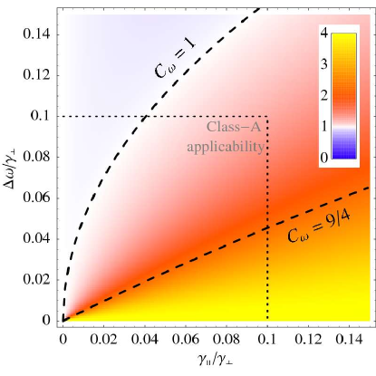
Figure 2: (Color online) The dependence of $C_{\omega}$ in Eq. (35) on $\gamma_{\parallel}$ and $\Delta\omega$. The dashed lines are the isolines for $C_{\omega}=1$ and $C_{\omega}=9/4$. The dotted lines approximately mark the applicability limits of class-A equations.

The dependence of $C_{\omega}$ is shown in Fig. 2. We can see that $C_{\omega}\lesssim 4$ for $\Delta\omega\ll\gamma_{\parallel}$ and $C_{\omega}\simeq 1$ for $\gamma_{\parallel}<\Delta\omega\ll\gamma_{\perp}$. The transition between two limiting cases ($C_{\omega}=1$ and $C_{\omega}=4$) occurs rapidly around $\Delta\omega\simeq\gamma_{\parallel}$. Note that as $\Delta\omega$ increases, $C_{\omega}$ approaches unity from below, so there is a critical value $\Delta\omega^{(1)}\approx\sqrt{\gamma_{\perp}\gamma_{\parallel}}/2$ for which $C_{\omega}=1$. Hence, in the ideal case of intensity matched modes [Eq. (18)] bistability is possible for $\Delta\omega$ all the way up to $\Delta\omega^{(1)}$. The limiting case of $C=4$ is known to be realized for the ideal case of counterpropagating modes in ring lasers or modes with orthogonal polarizations, which are fully intensity matched and have $\Delta\omega\approx 0$ Siegman .

If, however, the modes are considerably mismatched, then $C_{\omega}$ must be significantly larger than one to compensate for a small $C_{\alpha}$ and thus keep the overall mode coupling constant above unity to achieve bistable lasing. For example, it can be shown that 1D harmonic (e.g., longitudinal) modes always have $C_{\alpha}=4/9$ for different frequencies. This means that the line of critical values for $\Delta\omega^{(9/4)}\approx\gamma_{\parallel}/2$ up to where bistability is possible lies much deeper than the line of $\Delta\omega^{(1)}$ (see Fig. 2). Taking into account that the frequency shift between longitudinal modes is related to the cavity length as $\Delta\omega_{\textrm{(bulk)}}=\pi c/L$, one easily obtains the “rule of thumb” for minimum cavity length of a 1D bistable bulk laser: $L_{\textrm{min}}\simeq 2\pi c/\gamma_{\parallel}$. For realistic laser media, $L_{\textrm{min}}$ is found to be prohibitively large, from around 2 m for semiconductors and up to 200-300 km for Nd:YAG Svelto . This explains why it is so difficult to achieve bistable lasing for different-frequency modes in a bulk cavity: unless the cavity is extraordinary big, $\Delta\omega$ is large enough to bring $C_{\omega}$ so close to unity that any intensity mismatch causes $C_{\alpha}<1$ and brings the laser back into the weak-coupling (simultaneous lasing) regime. The only notable exception is the case when the modes are quasi-degenerate with $\Delta\omega\approx 0$, such as counterpropagating modes in ring lasers or modes with orthogonal polarization, and it is in these special cases that bistability could indeed be observed.

In a microcavity, however, the modes can be made very nearly intensity matched by a carefully chosen resonator design (e.g., coupled cavity-based, see zhukPRL ). In addition, many designs allow to control the frequency separation between the modes more or less independently from other model parameters. This opens up a whole new frequency range $\Delta\omega^{(9/4)}<\Delta\omega<\Delta\omega^{(1)}$ available for bistable laser design, which can encompass several orders of magnitude for $\Delta\omega$ (see Fig. 2). This range becomes available in microlasers because the possibility to bring the modes to intensity matching is far greater than in bulk cavities, owing to a greater variety of cavity shapes and a more complicated nature of the modes involved.

Finally, from Eqs. (31) one can also see the physical mechanism of bistable lasing in the class-A case. It is due to the (oscillatory) component $W_{12}$ that there is an addition to the cross-saturation coefficients $\theta_{ij\neq i}$. Without this addition, $C$ would simply coincide with $C_{\alpha}$ and all possibility for bistable operation would be excluded. Hence, it is the coherent mode interaction effects such as population pulsations or four-wave mixing LambLaser that make bistability possible. Incoherent effects (e.g., spatial hole burning, which is only manifest in $C_{\alpha}$) can either allow or suppress it. As a result, an interplay between coherent and incoherent mode interaction processes is employed to achieve bistable microlaser operation.

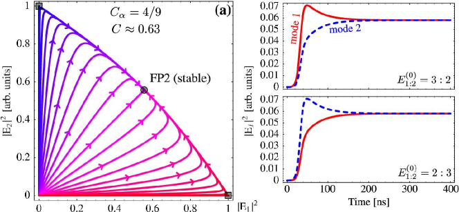
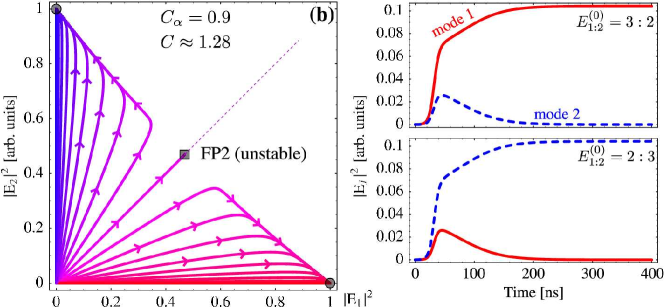
Figure 3: (Color online) Flow diagrams of numerical solutions of Eqs. (31) in the $\left|E_{1}\right|^{2}\textrm{ vs. }\left|E_{2}\right|^{2}$ plane for different initial mode ratios $E_{1:2}^{(0)}=\left|E_{1}(0)\right|:\left|E_{2}(0)\right|$ for (a) poorly matched modes ($C_{\alpha}=4/9$) and (b) well-matched modes ($C_{\alpha}=0.9$). The other parameters are the same ($\Delta\omega=\gamma_{\parallel}=10^{-2}\gamma_{\perp}$, $\kappa_{1}=\kappa_{2}=10^{-4}\gamma_{\perp}$), chosen such that $1<C_{\omega}<9/4$. Solid circles and squares denote stable and unstable fixed points, respectively. The thin dashed line denotes the separatrix in the bistable lasing case. The right panels show the example mode dynamics $\left|E_{1,2}(t)\right|^{2}$ for two chosen values of $E_{1:2}^{(0)}$ slightly in favor of each mode.

As an example, we have plotted the dynamics of mode amplitudes $E_{j}(t)$ as a numerical solution of Eqs. (31) for bulk-cavity ($C_{\alpha}=4/9$) vs. coupled-cavity ($C_{\alpha}=0.9$) modes (Fig. 3). Also shown are the temporal flow diagrams (i.e., projections of the solutions onto the $\left|E_{1}\right|^{2}\textrm{ vs. }\left|E_{2}\right|^{2}$ plane for different initial conditions of the cavity (the ratio $E_{1:2}^{(0)}\equiv\left|E_{1}(0)\right|:\left|E_{2}(0)\right|$). All other parameters are kept constant, as described in the caption. If the modes are mismatched (Fig. 3a) and $C<1$, the laser saturates to the two-mode simultaneous lasing ($\left|E_{1}\right|=\left|E_{2}\right|=\textrm{const}$) regardless of the initial conditions. Only this fixed point is stable. However, if the modes are well matched (Fig. 3b) so that $C>1$, the laser saturates to a single-mode lasing as the initially stronger mode quenches its weaker counterpart and becomes dominant. There are two stable fixed points on the diagram: $\left|E_{1}\right|=\textrm{const},\;\left|E_{2}\right|=0$ and $\left|E_{1}\right|=0,\;\left|E_{2}\right|=\textrm{const}$. The previously stable fixed point becomes unstable, and the line $\left|E_{1}\right|=\left|E_{2}\right|$ marks the separatrix between the stable points’ domains of attraction. The mode that has an advantage in the beginning determines the domain of attraction for the system and hence the fixed point the system will converge to, as the separatrix cannot be transcended without an external influence. These examples show that bistable lasing is possible in microlasers in such cases where only two-mode simultaneous lasing can be observed for bulk-cavity modes.

III.3 Conditions for bistable lasing: Mode mismatch

Up to now, we assumed that none of the modes is favored either by the cavity or by the gain, i.e., $\kappa_{1}=\kappa_{2}$, $R_{1}=R_{2}$, $\alpha_{11}=\alpha_{12}$, and $\delta_{\omega}=0$. In this case, as seen in Fig. 3, the two-mode lasing fixed point (labeled FP2), whether stable or unstable, is characterized by $\left|E_{1}\right|=\left|E_{2}\right|$. This means, on the one hand, that in the simultaneous-lasing case both modes lase with equal intensity (Fig. 3a), and on the other hand, that in the bistable regime even a slight edge given to either mode in terms of initial conditions will bring this mode to lase. It is equally easy to “select” or “switch” either mode by locking into it zhukPRL ; zhukPSS . This is illustrated in Fig. 3b by the fact that each stable fixed point has an equally large domain of attraction.

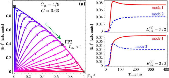
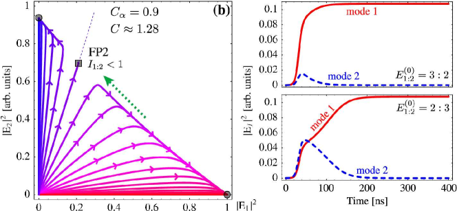
Figure 4: (Color online) Same as Fig. 3 for mismatched mode decay rates ($\kappa_{1}<\kappa_{2}$, $\delta_{\kappa}=-0.42\%$) in favor of the first mode. The dotted arrows show the shift of the two-mode fixed point FP2.

In a more general case, the ratio between mode intensities at FP2 $I_{1:2}\equiv\left|E_{1}\right|^{2}/\left|E_{2}\right|^{2}$ will change to reflect an advantage given to either of the modes. For example, even a slight mismatch in the mode $Q$-factors causes $I_{1:2}$ to deviate from unity (Fig. 4). Similar to the explanation given above, this may mean two things. In the simultaneous-lasing case, it simply means that once the laser achieves saturation, one mode has a greater amplitude than the other, e.g., $\left|E_{1}\right|>\left|E_{2}\right|$ for $I_{1:2}>1$ (Fig. 4a). In the bistable case, it means that the domains of attraction for the two modes change their size in phase space (Fig. 4b). If for example $I_{1:2}<1$, then the domain of attraction for Mode 1 becomes larger, so Mode 1 is “in favor” as a result. In the bistable regime, a shifted FP2 means that the mode with a smaller domain of attraction is out of favor and thus harder to bring to lasing. For example, if FP2 is placed symmetrically, initial mode amplitude ratios $E_{1:2}^{(0)}$ of 3:2 and 2:3 bring the first and the second mode to lasing, respectively (Fig. 3b). For asymmetrically placed FP2, the same two cases for initial condition both result in the lasing of the first mode (Fig. 4b). To be able to target the smaller domain, one has to excite the out-of-favor mode exclusively, which might be difficult experimentally. Hence we will further aim at finding the manifold of the system parameters for which $I_{1:2}=1$.

Whenever $C\neq 1$, the general expression for the mode intensity ratio at FP2 $I_{1:2}$ can be written as Siegman

$$I_{1:2}=\frac{\textrm{Re\,}\rho_{1}\textrm{Re\,}\theta_{22}-\textrm{Re\,}\rho_{2}\textrm{Re\,}\theta_{12}}{\textrm{Re\,}\rho_{2}\textrm{Re\,}\theta_{11}-\textrm{Re\,}\rho_{1}\textrm{Re\,}\theta_{21}}.$$ (36)

By substituting the coefficients in Eqs. (31) one can obtain an explicit analytic expression for $I_{1:2}$. Unfortunately, this general expression is very bulky and we will first investigate its behavior in several simplified cases. Let us introduce the perturbations in the form

$$\kappa_{1,2}\equiv\kappa(1\pm\delta_{\kappa}),\quad R_{1,2}\equiv R(1\pm\delta_{\alpha}),$$ (37)

from where it follows [see Eqs. (9) and (11)] that $\alpha_{11,22}=\alpha(1\pm\delta_{\alpha})^{2}$. Now if $\delta_{\omega}=\delta_{\alpha}=0$, $\delta_{\kappa}\neq 0$, $I_{1:2}$ is given by:

$$I_{1:2}^{(\kappa)}=\frac{a_{\kappa}+b_{\kappa}\delta_{\kappa}}{a_{\kappa}+b_{\kappa}\delta_{\kappa}}.$$ (38)

Likewise if $\delta_{\omega}=\delta_{\kappa}=0$, $\delta_{\alpha}\neq 0$, then the expression is somewhat more complicated and reads:

$$I_{1:2}^{(\alpha)}=\frac{\left(a_{\alpha}+c_{\alpha}\delta_{\alpha}^{2}+e_{\alpha}\delta_{\alpha}^{4}\right)+\left(b_{\alpha}+d_{\alpha}\delta_{\alpha}^{2}\right)\delta_{\alpha}}{\left(a_{\alpha}+c_{\alpha}\delta_{\alpha}^{2}+e_{\alpha}\delta_{\alpha}^{4}\right)-\left(b_{\alpha}+d_{\alpha}\delta_{\alpha}^{2}\right)\delta_{\alpha}}.$$ (39)

Finally, if if $\delta_{\alpha}=\delta_{\kappa}=0$, $\delta_{\omega}\neq 0$, then

$$I_{1:2}^{(\omega)}=\frac{\left(a_{\omega}+c_{\omega}\delta_{\omega}^{2}+e_{\omega}\delta_{\omega}^{4}\right)+\left(b_{\omega}+d_{\omega}\delta_{\omega}^{2}+f_{\omega}\delta_{\omega}^{4}\right)\delta_{\omega}}{\left(a_{\omega}+c_{\omega}\delta_{\omega}^{2}+e_{\omega}\delta_{\omega}^{4}\right)-\left(b_{\omega}+d_{\omega}\delta_{\omega}^{2}+f_{\omega}\delta_{\omega}^{4}\right)\delta_{\omega}}.$$ (40)

The coefficients in Eqs. (38)–(40) are complicated polynomial functions of the dynamical parameters $\gamma_{\perp}$ and $\gamma_{\parallel}$, the intermode frequency separation $\Delta\omega$, the measure of mode intensity mismatch $\nu\equiv\alpha_{12}/\alpha$ (which ranges from 0 to a maximum value of $1-\delta_{\alpha}^{2}$ so that $C_{\alpha}\leq 1$), and the pumping rate normalized to the threshold pumping $R_{\textrm{thr}}\equiv 2Rg\omega/(\gamma_{\perp}\kappa)$ . Note that $\kappa$ itself does not enter these equations explicitly. It does, however, impose a limitation $\Delta\omega>10^{-2}\kappa$ so that the phase terms in Eqs. (27) can be averaged out.

From the structure of Eqs. (38)–(40) one can see that $I_{1:2}=1$ for $\delta_{\alpha}=\delta_{\kappa}=\delta_{\omega}=0$, as should be expected. If any one of the perturbation parameters ($\delta_{\omega,\kappa,\alpha}$ collectively referred to as $\delta$) is non-zero, $I_{1:2}$ deviates from unity. Obviously, changing the sign of all non-zero $\delta$ causes $I_{1:2}\to 1/I_{1:2}$. If favoring one of the modes (by any means) results in a certain asymmetry in lasing quantified through a non-unity $I_{1:2}$, then favoring the other mode in the same way and by the same amount naturally causes the same asymmetry with respect to the other mode . This suggests that one can choose more than one $\delta$ to be non-zero in such a way that the shifts of FP2 caused by individual perturbations would cancel each other out. As a result, one could achieve the resulting $I_{1:2}$ equal to or close to unity, and the restrictions on the initial conditions would be lifted.

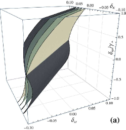
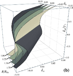
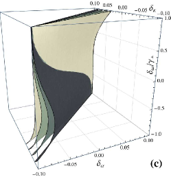
Figure 5: (Color online) Manifolds of points $I_{1:2}=1$ in the 3D perturbation space $(\delta_{\omega};\delta_{\kappa};\delta_{\alpha})$ for (a) $C=1.10\gtrsim 1$, (b) $C=2.06\simeq 2$, and (c) $C=3.84\lesssim 4$. The four surfaces correspond to four values of the pumping rate ($R/R_{\textrm{thr}}=1,1.25,1.5,1.75$), as indicated in the panel (b).

Fig. 5 shows the manifold of the points $I_{1:2}=1$ in the 3D perturbation space $(\delta_{\omega};\delta_{\kappa};\delta_{\alpha})$ for different parameters as a numerical solution of Eq. (36). We can see that this manifold is an open surface. Hence, if a mismatch in one respect is unavoidable, it can be compensated for by engineering the other two perturbation parameters. Note that in the $(\delta_{\kappa};\delta_{\alpha})$ plane the mismatch compensation ($I_{1:2}=1$) is achieved when $\delta_{\kappa}\approx\delta_{\alpha}$. This is easily understood if one remembers that the linear terms in Eqs. (27) have the structure $\rho_{j}\sim\zeta R_{j}-\kappa_{j}=\zeta R(1\pm\delta_{\alpha})-\kappa(1\pm\delta_{\kappa})$. On the other hand, in the $(\delta_{\omega};\delta_{\kappa})$ plane, compensation is generally achieved for the oppositely-signed $\delta_{\omega}$ and $\delta_{\kappa}$. This is in agreement with an intuitive guess that, e.g., $\delta_{\kappa}<0$ ($\kappa_{1}<\kappa_{2}$) and $\delta_{\omega}<0$ (the gain frequency $\omega_{a}<\omega_{0}$ is closer to $\omega_{1}$ than to $\omega_{2}$, see Fig. 1) both give an edge to the first mode, so oppositely-signed $\delta$ are needed to maintain balance. However, in the vicinity of the origin the surface can be folded, so that it crosses the origin with the opposite slope and compensation is achieved when $\delta_{\omega}$ and $\delta_{\kappa}$ have the same sign. Since perturbations $\delta_{\omega}$, $\delta_{\alpha}$, and $\delta_{\kappa}$ can have different physical origin and can be varied more or less independently by a proper choice of a gain medium and a cavity configuration, one can deliberately engineer a microlaser to achieve bistable operation even if the idealized, unperturbed case is difficult to realize experimentally. An example of such compensation is changing the mode frequencies with respect to gain (which can be done straightforwardly just by scaling the cavity) to help offset the difference in mode $Q$-factors, as shown numerically in our earlier work zhukPSS .

To achieve a fully symmetric placement of FP2, one needs to bring three perturbation parameters into a relation. Because all these parameters show only an indirect dependency on the cavity design and/or gain medium choice, the precise control of them may still be a challenging task. Hence, it is worthwhile to investigate to what extent the relations for ideal compensation can be violated so that bistable operation is still possible (albeit, as shown above, at the cost of stricter requirements on the initial conditions). In terms of Fig. 5, that means how far one can deviate from the $I_{1:2}=1$ surface and still lase into either of the modes on demand.

From Eqs. (38)–(40) one sees that a sufficiently high value of any $\delta$ will cause either the numerator or the denominator in $I_{1:2}$ to approach zero. On the flow diagram, this corresponds to the FP2 meeting the coordinate axes. Increasing $\delta$ further causes $I_{1:2}$ to become negative. The FP2 vanishes and the system finds itself in the single mode lasing regime (see Siegman ). That sets an upper limit for any $\left|\delta\right|$ beyond which no bistable lasing is possible any more.

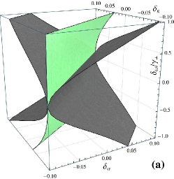
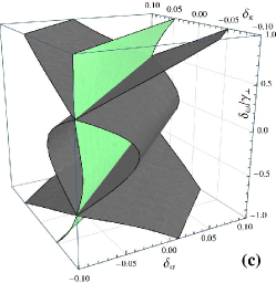
Figure 6: (Color online) Boundaries of the FP2 existence domain $I_{1:2}>0$ (dark gray) and the $I_{1:2}=1$ surface lying inside that domain (light green) for $C\lesssim 4$ (as in Fig. 5c): (a) at threshold ($R/R_{\textrm{thr}}=1$), (b) 10% above threshold ($R/R_{\textrm{thr}}=1.2$), and (c) 20% above threshold ($R/R_{\textrm{thr}}=1.2$).

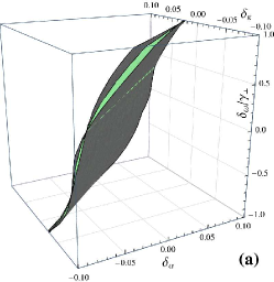
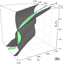
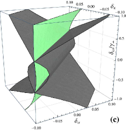
Figure 7: (Color online) Same as Fig. 6 for constant $R$ at 10% above threshold and (a) $C\gtrsim 1$, (b) $C\simeq 2$, (c) $C\lesssim 4$, corresponding to the cases in Fig. 5a–c.

More generally, the domain in space $(\delta_{\omega};\delta_{\kappa};\delta_{\alpha})$ where $I_{1:2}>0$ comprises the possible perturbation parameter window where both modes can lase (either simultaneously or subject to bistability-induced switching, as depends on $C$). This domain, called the FP2 existence domain, is shown in Figs. 6–7. The existence domain, bounded by the surfaces defined by $I_{1:2}=0$ and $I_{1:2}=\infty$ is seen to surround the “perfect matching” surface $I_{1:2}=1$. The domain boundaries appear to slide inwards as the pumping rate increases (Fig. 6), which enlarges the FP2 existence domain around the point $\delta=0$. Also, the domain shrinks rapidly as the boundaries close around $I_{1:2}=1$ when $C$ approaches unity (Fig. 7). The latter can be intuitively understood because $C\approx 1$ represents a delicately balanced system, so that even a slight mismatch is enough to throw the system heavily out of balance. Such a property is clearly a misfortune for the microcavity-specific bistability range reported above, as it relies on the situation when $C_{\omega}$ exceeds unity only slightly. However, increasing the pumping appears to counteract this disadvantage, at least for smaller $\delta_{\omega}$ (see Fig. 6). We believe that it is this effect that enabled us to observe bistability in earlier numerical simulations zhukPRL ; zhukPSS involving the laser operating highly above threshold.

The practical conclusion to this section is that there are two theoretical requirements needed to achieve bistable lasing. In the first place, FP2 needs to exist on the flow diagram, as imposed by $I_{1:2}>0$. In the second place, once FP2 exists, the mode coupling constant must exceed unity ($C>1$), as discussed before. First (Sec. III.2), we have shown that in comparison to bulk-cavity lasers microlasers exhibit a much wider parameter window characterized by $C>1$, because the microcavity modes can better fulfill the intensity matching condition (18). Secondly (Sec. III.3), we have shown that there is an extended domain in the 3D perturbation space $(\delta_{\omega};\delta_{\kappa};\delta_{\alpha})$ where $I_{1:2}>0$. Inside this domain, the closer $I_{1:2}$ is to unity, the easier it is to realize bistability-based laser mode switching experimentally. We have shown that $I_{1:2}$ can be brought close to 1 by choosing a combination of perturbation parameters that would compensate each other’s advantage given to either mode.

IV Class-B/C microlasers

The elegance of the class-A case considered in the previous section is that Eqs. (27) can be subject to analytical investigation based on a comparison with Eqs. (28) Siegman . Once a laser with a more complicated dynamics needs to be examined, more complicated systems of equations [six equations (13)–(14) for class-B or eight equations (7)–(10) for class-C] need to be dealt with. Although attempts at analytical investigation of class-B equations are known (e.g., a near-threshold expansion of population inversion as proposed in mcZehnle ), only numerical solution seems to be applicable in the general case when no specific assumptions on the cavity or mode geometry are implied. Since all the equations are ordinary differential, such a numerical solution can be carried out with relative ease – the computational demands are far lower than a direct numerical integration of the Maxwell-Bloch equations by means of an FDTD-like scheme zhukFDTD .

A systematic investigation of class-B/C microlasers would be too lengthy to include in the present paper and will be the subject of a forthcoming publication. In this section we will outline the main differences in the behavior of such lasers compared to the previously studied class-A case as regards bistable lasing.

We begin with a comparison of the laser classes in the near-threshold regime. As should be expected, the solutions for all classes display full coincidence if the class-A approximation $\gamma_{\perp}\gg\gamma_{\parallel}\gg\kappa$ holds (note that this condition is rather restrictive in microlasers, requiring a careful choice of the gain medium as well as the cavity design). The mode dynamics $E_{j}(t)$ start to exhibit differences whenever $\gamma_{\parallel}$ or $\kappa$ are increased out of the class-A approximation. The differences, however, are relatively minor, manifesting themselves mainly in the character of the transition process. In most cases, the mode coupling constant $C$ as defined for the class-A in Eqs. (33)–(35) continues to predict the laser dynamics correctly ($C<1$: simultaneous lasing, $C>1$: bistability) even outside its strict range of applicability, although the behavior of $E_{j}(t)$ can be quite different during the transition period.

As discussed above, the class-B equations (13)–(14) do not involve a near-threshold approximation, it becomes possible to consider a greater range of pumping rates, including regimes far above threshold, which are often left out of the picture in a construction of a multimode laser model mcHodges . Comparison of the numerical results for class-B vs. class-C equations show that as long as the class-B prerequisites $\gamma_{\perp}\gg\gamma_{\parallel},\kappa_{j}$ hold, the results are similar, unless the condition $\gamma_{\perp}\gg\Delta\omega$ is violated. This agrees well with the earlier discussions in Section II.3. The differences appear not to be qualitative, but quantitative only, manifesting in the exact shape of the $\left|E_{j}(t)\right|$ dependence. The overall outcome of the mode interaction largely remains the same. To summarize, the main effect of the class-A to class-B transition in the context of studying bistable lasing is the inclusion of larger pumping rates $R$, while the main effect of the class-B to class-C transition is the inclusion of larger frequency mode separations $\Delta\omega$.

The increase of the pumping rate in a class-B laser is known to change the saturation character of the mode amplitudes. The non-instantaneous relaxation of the population inversion with respect to the cavity field gives rise to spiking (for smaller $R$) or relaxation oscillations (for greater $R$) in the dependence $E_{j}(t)$. A still stronger pumping (several orders of magnitude above threshold) causes the oscillations to vanish, as reported in an earlier work zhukFDTD .

More interestingly, an increase of $R$ can restore bistable lasing in the cases when simultaneous lasing is observed just above threshold. Fig. 2 suggests that there should be no bistability in the area around $\Delta\omega\simeq\gamma_{\perp}$. The numerical solution of the class-C equations shows that this is indeed the case for smaller $R$. However, if the pumping is increased beyond a certain critical value $R_{c}$, a transition from simultaneous to bistable lasing occurs (Fig. 8). This effect was reported earlier zhukFDTD with the observation that bistability ensues when pumping becomes so large that relaxation oscillations disappear. Our further investigations have revealed that this observation was rather a coincidence, and $R_{c}$ scales with $\Delta\omega$ (Fig. 8), bifurcating from threshold at approximately the point where $C_{\omega}=1$ according to Eq. (35). This falls in line with the result of the previous section that a stronger pumping is capable of restoring bistability where it has been deteriorated by adverse effects of insufficient mode matching.

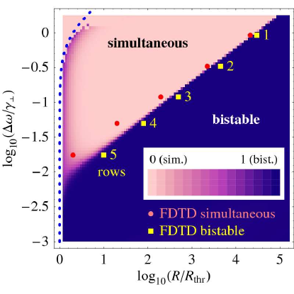
Figure 8: (Color online) The dependence of lasing regime on pumping rate $R$ and intermode frequency separation $\Delta\omega$ in a class-C laser model. The parameters are $\kappa_{j}\simeq 0.1\gamma_{\perp}$ and $\gamma_{\parallel}\simeq 10^{-4}\gamma_{\perp}$, as used for numerical simulation in zhukPRL . The density plot shows the quantity $\left|\left|E_{1}(t)\right|-\left|E_{2}(t)\right|\right|/\max\left(\left|E_{1}(t)\right|,\left|E_{2}(t)\right|\right)$ for large $t\gg\gamma_{\perp}^{-1},\gamma_{\parallel}^{-1},\kappa_{j}^{-1}$. Near-zero (light) values indicate two-mode (simultaneous) lasing while near-unity (dark) values indicate one-mode (bistable) lasing. The lasing threshold depending on $\Delta\omega$ is marked with the dotted line. Numerical results of the FDTD simulations for coupled-defect structures (Fig. 9) are superimposed over the density plot. Circles (red) and squares (yellow) show the location of points where simultaneous and bistable lasing, respectively, was observed in the mode dynamics during simulations.

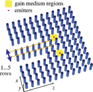
Figure 9: (Color online) The family of structures used in numerical FDTD simulations, based on two coupled defects in a 2D photonic crystal lattice zhukPRL ; zhukFDTD . Placing a different number of lattice rows between the defects (1–5), the intermode frequency separation $\Delta\omega$ can be changed.

Because applicability of the expansion (5) and sometimes even of the SVEA TureciOE may become questionable far above threshold, we have carried out a comparison of Class-B/C results with direct numerical simulations. As previously described in Ref. zhukFDTD , a space-time FDTD solver was coupled to the four-level laser rate equations in order to model the response of a laser medium. A 2D photonic crystal lattice with two coupled defects zhukPRL was used as a model system (Fig. 9). Both defects are filled with four-level gain medium and contain a dipole source in the centre . By exciting these sources with varying amplitude/phase relations, the two modes (symmetric and antisymmetric zhukFDTD ) can be excited in any proportion and thus the initial state of the resonator can be controlled. By changing the number of lattice rows between the defects from 1 to 5, one can change $\Delta\omega$ from $\sim\gamma_{\perp}$ down to $\sim 10^{-2}\gamma_{\perp}$ . The waveguides coupled to the defects form the primary channel for the radiation to leak out of the resonator. Care was taken that the mode $Q$-factors remain approximately the same across the whole family of structures.

The results of the FDTD simulation runs are superimposed in the phase diagram in Fig. 8. For all values of $\Delta\omega$, the transition between simultaneous and bistable lasing was found approximately around $R_{c}$ as predicted by the analytical theory. For larger $\Delta\omega$ the correspondence is better because smaller $\Delta\omega$ and $R$ require much longer times to get to the steady state and there is an increased sensitivity to mode mismatch (see Fig. 6). Hence it becomes more difficult to establish the transition point between simultaneous and bistable lasing with good accuracy.

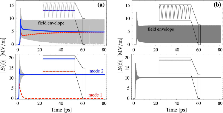
Figure 10: (Color online) Comparison between laser field dynamics obtained by (a) the Class-C equations and (b) direct FDTD numerical simulations for the 2D PhC structure (see Fig. 9) with defects separated by 2 lattice rows (point #2 in Fig. 8, $\log_{10}\left[\Delta\omega/\gamma_{\perp}\right]=-0.481$) for $R<R_{c}$ (top) and $R>R_{c}$ (bottom). For the Class-C coupled mode theory results, the red dashed and blue solid lines show the mode amplitudes $\left|E_{1,2}(t)\right|$, respectively. Initially both modes are excited and the second mode is given an advantage ($E_{1:2}^{(0)}=2:3$). The gray line shows the electric field at the mode’s maximum $\left|E_{r}(t)\right|=u_{\text{max}}\left|E_{1}(t)\mathrm{e}^{\phi_{+}}+E_{2}(t)\mathrm{e}^{\phi_{-}}\right|$. For the FDTD results, the field envelope at the center of either defect $\left|E(\mathbf{r}_{c},t)\right|$ is shown (sampled at local extrema of light oscillations). The insets show an enlarged portion of the plots to show the $2\Delta\omega$ intermodal beating whenever both modes lase at the same time.

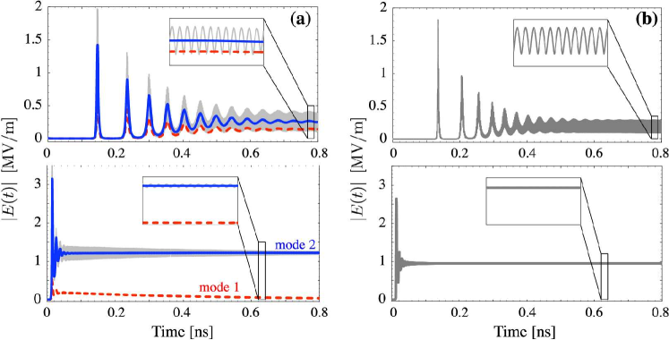
Figure 11: (Color online) Same as Fig. 10 but for the 2D PhC structure with defects separated by 4 rows (point #4 in Fig. 8, $\log_{10}\left[\Delta\omega/\gamma_{\perp}\right]=-1.301$).

In Figs. 10 and 11, temporal laser dynamics in numerical simulations and the Class-C model are compared. We analyze the electric field in the center of either defect $\mathbf{r}_{c}$. For FDTD, it is monitored directly by recording the field at the corresponding point in space $E(\mathbf{r}_{c},t)$. To reduce the excessive amount of data, we sample the field only at the local maxima, so that an envelope over the light oscillations is plotted. In the case of the coupled mode theory, the same quantity is obtained from the mode amplitudes $E_{1,2}(t)$ using Eq. (4) as $E_{r}(t)=u_{\text{max}}\left(E_{1}(t)\mathrm{e}^{-\mathrm{i}\omega_{1}t}+E_{2}(t)\mathrm{e}^{-\mathrm{i}\omega_{2}t}\right)$ where $u_{\text{max}}=\max\left[u(\mathbf{r})\right]$, assuming the modes are normalized according to Eq. (6). Taking the absolute value, light oscillations are also neglected, so the results can be compared to the simulations.

In all examples of Figs. 10, 11 (which correspond to the laser operating way above threshold), the field dynamics shows a good qualitative and quantitative correspondence. Below $R_{c}$ where simultaneous two-mode lasing is expected, the in-cavity field envelope shows the characteristic $2\Delta\omega$ beat oscillations (see the insets in Figs. 10–11), marking the presence of both modes in the laser radiation. Above $R_{c}$, the steady-state envelope is flat, indicative of single-mode lasing, and the beat oscillations are seen to vanish. This corresponds to quenching of the weaker mode in agreement with theoretical expectations in the bistable regime.

Some quantitative discrepancies between the model and simulation results can be noticed. Some of them (e.g., temporal shifts of the spikes in Fig. 11) result from minor deviations in parameters between the real simulated structure and an idealized two-mode system considered. These deviations can be compensated for by fine-tuning the model zhukFDTD . Other discrepancies such as the the difference in the field amplitudes (both at spike maxima and in the steady-state) can be attributed to gain saturation, which may introduce correction to the form of the expansion (5) for the gain medum polarization. This is a limitation inherent in the present coupled-mode model. However, Eqs. (7)–(10) and (13)–(14) are clearly seen to provide a valid description of laser mode dynamics scenario for relatively strong pumping, unlike the near-threshold (third-order nonlinearity) theories which are reported to fail badly in this regime (see Tureci06 ), just like the Class-A equations (31) would. One can overcome this limitation, e.g., following the approach in Refs. Tureci06 ; Tureci07 where a generalization of Eqs. (4)–(5) is introduced. A very good agreement with numerics is reported recently TureciOE . However, only the time-independent (steady-state) theory is formulated so far.

The knowledge that stronger pumping can restore a laser into the bistable regime for higher $\Delta\omega$ is important in the design of a laser that can have its wavelength switched by a large value (such as several tens of nanometers in Refs. zhukPRL ; zhukPSS ) . A rigorous explanation of this result is yet to be given. Intuitively, stronger pumping rates cause shorter lasing onset times compared to the cavity round-trip time, so the domination of the stronger mode can occur before the modes have a chance to balance themselves through the cavity. Indeed, it could be noticed that the transition from simultaneous to bistable lasing around $R_{c}$ is accompanied by the disappearance of $4\Delta\omega$-pulsations in the phase of some dynamical variables. This suggests that shorter onset due to stronger pumping allows some of the variables to become phase-locked, which in turn influences the whole character of the mode interaction (as was seen when the transition from Eq. (27) to Eq. (31) was discussed). The detailed investigation of this effect is a subject for further studies.

V Conclusions and outlook

In this work, we have addressed the problem of bistability in a microlaser by systematically formulating the coupled-mode model without prior assumptions on the mode or cavity geometry, other than the requirement of the mode orthogonality in the cavity as well as in the gain region as described by Eqs. (6) and (15). The governing equations have been derived for all laser classes, Eqs. (7)–(10), (13)–(14), and (27) for class-C, B, and A, respectively. The issue of classifying the laser dynamics in the multimode case has been revisited taking into account the intermode frequency separation $\Delta\omega$ as a new parameter influencing the laser dynamics. The model has been derived for the case of two modes; however, its extension to the case of several modes can be performed along the same lines.

The simplest case of the class-A laser equations has been analytically investigated. It has been shown that coherent mode interaction processes (population pulsations) can provide an additional mode coupling channel besides incoherent mode interaction (spatial hole burning). This additional coupling is what brings the laser into the bistable regime, allowing the lasing mode to be chosen on demand by the initial condition of the cavity. This result agrees with the early theoretical predictions Siegman ; LambLaser . However, microcavity modes can have a far better matched intensity distribution inside the gain region, see Eq. (18), compared to bulk-cavity modes, which are usually heavily out of match unless $\Delta\omega=0$. As such, only a moderate amount of pulsation-induced mode coupling is enough to enter the bistability regime in the case of a microlaser. This means that microlasers can be bistable in a far greater parameter range than bulk-cavity lasers, e.g., for much larger $\Delta\omega$ (Fig. 2). We have also shown that a sizable mismatch in the system parameters that favors one of the modes can destroy any chance of bistable operation. However, a mismatch with respect to one parameter can be compensated for by a mismatch with respect to another (Fig. 5). Again, due to better matched intensity distributions of microcavity modes the bistable regime is more tolerant to such perturbations (Fig. 7).

In the more general class-B or class-C laser models, we have shown numerically that even when $\Delta\omega$ is too large to allow bistability in the near-threshold class-A case, it can be overcome by increasing the pumping rate (Fig. 8). The results of the theory are confirmed by direct numerical FDTD simulations and are shown to be qualitatively valid for pumping rates several orders of magnitudes above the lasing threshold. Further results on bistability in class-B/C microlasers will be available in a forthcoming publication.

Bistable operation of a multimode microlaser can be useful in many respects. Since there is no need for an external (and potentially slow) cavity-tuning process, ultrafast all-optical mode switching mechanisms can be imagined. Such switching, occurring across $\simeq 20$ nm on a picosecond time scale had indeed been demonstrated numerically in our earlier work zhukPRL . The fast switching between stable states and the relatively low power of microlasers can be used in the design of an optical memory (flip-flop) cell. We believe, that a compact-sized microlaser capable of multiple-wavelength operation in a wide wavelength range can find numerous applications in integrated optics and optical communication.

- (1) K. J. Vahala, Nature 424, 839 (2003).
- (2) O. Painter, R. K. Lee, A. Scherer, A. Yariv, D. O’Brien, P. D. Dapkus, and I. Kim, Science 284, 1819 (1999).
- (3) M. Imada, A. Chutinan, S. Noda, and M. Mochizuki, Phys. Rev. B 65, 195306 (2002).
- (4) S. Ishii and T. Baba, Appl. Phys. Lett. 87, 181102 (2005).
- (5) M. Hill, H. Dorren, T. de Vries, X. Leijtens, J. Hendrik den Besten, B. Smalbrugge, Y.-S. Oei, H. Binsma, G.-D. Khoe, and M. Smit, Nature 432, 206 (2004).
- (6) A. Siegman, Lasers (University Science Books, Mill Valley, CA, 1986), Ch. 25.4.
- (7) M. Sargent III, M. O. Scully, and W. E. Lamb, Jr., Laser Physics (Addison-Wesley, Reading, MA, 1974), Ch. 9.
- (8) M. Sorel, P. J. R. Laybourn, A. Scirè, S. Balle, G. Giulliani, R. Miglierina, and S. Donati, Opt. Lett. 27, 1992 (2002).
- (9) C. L. Tang, A. Schremer, and T. Fujita, Appl. Phys. Lett. 51, 1392 (1987).
- (10) C.-F. Lin and P.-C. Ku, IEEE J. Quant. Electron. 32, 1377 (1996).
- (11) H. Kawaguchi, IEEE J. Sel. Top. Quant. Elecron. 3, 1254 (1997).
- (12) G. P. Agrawal and N. K. Dutta, J. Appl. Phys. 56, 664 (1984).
- (13) R. Kuszelewicz and J. L. Oudar, IEEE J. Quant. Electron. QE-23, 411 (1987).
- (14) S. W. Wieczorek and W. W. Chow, Phys. Rev. A 69, 033811 (2004).
- (15) S. W. Wieczorek and W. W. Chow, Opt. Commun. 246, 471 (2004).
- (16) M. Takenaka, K. Takeda, Y. Kanema, Y. Nakano, M. Raburn, and T. Miyahara, Opt. Express 14, 10785 (2006).
- (17) S. V. Zhukovsky, D. N. Chigrin, A. V. Lavrinenko, and J. Kroha, Phys. Rev. Lett. 99, 073902 (2007).
- (18) S. V. Zhukovsky, D. N. Chigrin, A. V. Lavrinenko, and J. Kroha, Phys. Stat. Sol. (b) 244, 1211 (2007).
- (19) S. Zhang, D. Lenstra, Y. Liu, H. Ju, Z. Li, G. D. Khoe, and H. J. S. Dorren, Opt. Commun. 210, 85 (2007).
- (20) H. E. Türeci, A. Douglas Stone, and B. Collier, Phys. Rev. A 74, 043822 (2006).
- (21) H. E. Türeci, A. Douglas Stone, and Li Ge, Phys. Rev. A 76, 013813 (2007).
- (22) H. E. Türeci, Li Ge, S. Rotter, and A. Douglas Stone, Science 320, 643 (2008).
- (23) S. E. Hodges, M. Munroe, J. Cooper, and M. G. Raymer, J. Opt. Soc. Am. B 14, 191 (1997).
- (24) L. Florescu, K. Busch, and S. John, J. Opt. Soc. Am. B 19, 2215 (2002).
- (25) S. V. Zhukovsky, D. N. Chigrin, Phys. Stat. Sol. (b) 244, 3515 (2007).
- (26) V. Zehnlé, Phys. Rev. A 57, 629 (1998).
- (27) H. Haken and H. Sauermann, Z. Phys. 173, 261 (1963);
- (28) H. Fu and H. Haken, Phys. Rev. A 43, 2446 (1991),
- (29) A. E. Siegman, Phys. Rev. A 39, 1253 (1989).
- (30) O. Svelto, Principles of lasers (Plenum Press, New York, 1989), Ch. 6.
- (31) Li Ge, R. J. Tandy, A. Douglas Stone, and H. E. Türeci, Opt. Express 16, 16895 (2008).