Detection methods of binary stars with low- and intermediate-mass components

Abstract

This paper reviews methods which can be used to detect binaries involving low- and intermediate-mass stars, with special emphasis on evolved systems. Besides the traditional methods involving radial-velocity or photometric monitoring, the paper discusses as well less known methods involving astrometry or maser (non-)detection. An extensive list of internet resources (mostly catalogues/databases of orbits and individual measurements) for the study of binary stars is provided at the end of the paper.

1 Scope of the paper

Binary stars are home to so many different physical processes that an exhaustive review of them would fill a thick textbook. It is therefore necessary to delineate right away the scope of the present text, which focuses on the methods to detect binaries. Besides the traditional methods involving radial-velocity or photometric monitoring, the discussion covers as well less known methods involving astrometry or maser (non-)detection. For a more traditional review focused on the evolutionary aspects (including a detailed description of the evolution of orbital elements), we refer the reader to the recent book by Eggleton (2006), or to the older Saas-Fee course (Shore, 1994).

Because of the authors’ own biases, this review on binary detection methods must be understood in the general scientific context of systems involving low- and intermediate-mass (’L&IM’) stars, i.e., stars which end their lifes as white dwarfs (WDs). For this reason, some of the detection methods discussed in the present review only apply to L&IM binary systems; conversely, methods that are specific to massive binaries (Wolf-Rayet binaries, High-mass X-ray binaries, binaries involving black holes or pulsars) will not be addressed here.

This review is organized as follows. The specificities of L&IM stars are briefly discussed in Sect. 2. Basic concepts about binaries (orbital elements and Roche lobe) are summarized in Sect. 3. Possible ways to detect binary systems (sometimes specific to L&IM binaries) are reviewed in Sects. 4 to 7, covering spectroscopic methods (Sect. 4), photometric methods (Sect. 5), astrometric methods (Sect. 6) and miscellaneous other methods (Sect. 7). We stress the difficulties associated with these methods. The reader is referred to a recent lecture by Halbwachs (http://www.astro.lu.se/ELSA/pages/PublicDocuments/Halbwachs.pdf) for a good introduction on the technical aspects of the main methods, and to the book Observing and Measuring Visual Double Stars (Argyle, 2004) for methods relating to visual binaries, which are not addressed here. A summary of what may be known about masses for the different kinds of binaries is presented in Sect. 8, and finally Sect. 9 provides an extensive list of internet resources (mostly catalogues/databases of orbits and individual measurements) for the study of binary stars.

2 The families of L&IM binaries

Figure 1: The evolution of a system consisting initially of two L&IM main-sequence stars. The left column corresponds to the normal evolutionary sequence of single stars, while the right column represents the various classes of stars with chemical peculiarities specifically produced by mass transfer across the binary system. Hatched circles denote stars with atmospheres enriched in carbon or heavy elements. (From (Jorissen, 2003a))

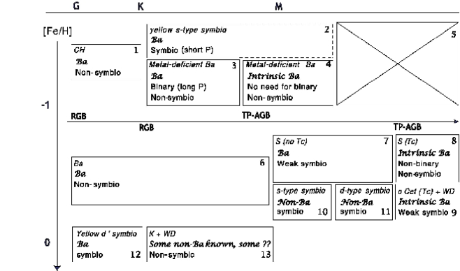
Figure 2: The various kinds of symbiotic stars (SyS) and of peculiar red giants, in a plane spectral-type vs. metallicity. Within each box, the first line (slanted font) lists the stellar family, the second line (calligraphic font) indicates whether or not stars from that family are enriched in s-process elements (either from internal nucleosynthesis – ”Intrinsic Ba” – or from mass transfer across a binary system – ”Ba” standing for Extrinsic Ba). The last lines (regular font) provide the binary properties of that family: binary (short or long periods) or non-binary, SyS or non-SyS. Each box has been assigned a number, for easy reference in the text. The horizontal line with an arrow in the middle of the figure is to indicate that the thermally-pulsing AGB phase (where the s-process nucleosynthesis takes place) involves different spectral types at low- and near-solar metallicity. (From (Frankowski and Jorissen, 2007))

What makes L&IM stars so interesting is that in the course of their evolution they go through the asymptotic giant branch (AGB) phase of evolution. AGB stars have two very important properties: they are home to a rich internal nucleosynthesis and exhibit strong mass loss. Besides controlling the AGB evolutionary timescale, the strong mass loss has important side effects when it occurs in a binary system, like the development of symbiotic activity, of associated X-ray emission, of maser emission (possibly suppressed by the perturbation induced by the companion), etc… In many ’after-AGB’ systems, the mass transfer from an AGB star has left its mark on the companion, enhancing its abundances with the products of the AGB nucleosynthesis, most remarkably C, F, and elements heavier than iron produced by the s-process of nucleosynthesis (see Lattanzio and Wood, 2003, for a recent review). An exemplary case of after-AGB systems are barium stars: G-K type giants remarkable for their overabundances of Ba (McClure, 1984). Related families include the Abell-35 subclass of planetary nebulae (Bond et al., 1993), barium dwarfs (including the so-called WIRRing stars; Jeffries and Stevens, 1996), subgiant and giant CH stars (McClure, 1984, 1997), extrinsic S stars, as opposed to intrinsic S stars, which exhibit spectral lines of the element technetium, a product of s-process nucleosynthesis which has no stable isotopes (Jorissen and Mayor, 1992) and d’-type yellow symbiotics (Schmid and Nussbaumer, 1993). But not all of the after-AGBs need to be s-process rich. The post-AGB binaries are an interesting case, as they are all by definition after-AGBs: some of them do exhibit s-process enhancement while others do not (Van Winckel, 2003, 2007). Neither do symbiotic stars (SyS) involving M giants and massive WD companions ($M_{WD}>0.5$ $M_{\odot}$) exhibit s-process enhancements (Jorissen, 2003b). Finally, some of the cataclysmic variables with massive WDs should also belong to the after-AGB family. An extensive list of families of binary stars with WD companions is presented in the dedicated reviews of Jorissen (2003a) and Parthasarathy et al. (2007). How the different families mentioned above fit in a coherent evolutionary scheme is sketched in Fig. 1.

While Fig. 1 provides a classification of L&IM binaries in terms of a temporal sequence, one may also try to order them in terms of their physical properties, like metallicity, spectral type and symbiotic activity. Symbiotic activity is expected when a compact star is heated by matter falling onto it from a mass-losing (often giant) companion. As it will be discussed in more details later on, the hallmark of SyS is a hot spectral continuum superimposed on cool spectral features, but symbiotic activity also means outbursts, X-ray emission, high-excitation emission lines, and nebular lines.

Fig. 2 is an attempt to classify L&IM binaries in the plane metallicity – spectral-type, and to correlate this location with the presence or absence of symbiotic activity (for reviews, see Frankowski and Jorissen, 2007; Jorissen, 2003b; Jorissen et al., 2005).

Metallicity, plotted along the vertical axis, has a strong impact on (i) the spectral appearance, which controls taxonomy (CH giants for instance – box 1 – are the low-metallicity analogs of the barium stars – box 6); (ii) the efficiency of heavy-element synthesis, being more efficient at low metallicities (Clayton, 1988), and (iii) the location of evolutionary tracks in the Hertzsprung-Russell diagram (hence the correspondence between spectral type and evolutionary status, like the onset of thermally-pulsing AGB, where the s-process operates, will depend on metallicity). Fig. 2 therefore considers three different metallicity ranges: (i) [Fe/H]$<-1$, corresponding to the halo population; (ii) $-1\leq$[Fe/H]$\leq 0$, or disk metallicity; (iii) [Fe/H]$\geq 0$, solar and super-solar metallicities found in the young thin disk.

The horizontal axis in Fig. 2 displays spectral type. At a given metallicity, spectral type is a proxy for evolutionary status: the giant components in L&IM binaries may either be located on the first red giant branch (RGB), in the core He-burning phase (which is hardly distinguishable from the lower RGB/AGB; CH giants probably belong to that phase), He-shell burning early AGB (E-AGB), or on the thermally-pulsing AGB (TP-AGB) phase, where the s-process operates.

Symbiotic activity is expected in the middle of this spectral sequence, because (i) at the left end, stars (like CH) are not luminous enough to experience a mass loss sufficient to power symbiotic activity; (ii) at the right end, the stars with the barium syndrome need not be binaries. Indeed, in TP-AGB stars, heavy-elements are synthesized in the stellar interior and dredged-up to the surface, so that “intrinsic Ba” (or S) stars occupy the rightmost boxes – 4 and 8 – of Fig. 2, and hence need not exhibit any symbiotic activity since they are single stars (For examples of stars belonging to box 4, see (Jorissen et al., 2005) and (Drake and Pereira, 2008)). Such evolved giants which are nevertheless members of binary systems (like Mira Ceti – box 9) will of course exhibit symbiotic activity. It is noteworthy that late M giants are inexistent in a halo population (hence the crossed box 5), because evolutionary tracks are bluer as compared to higher metallicities. Examples of such very evolved (relatively warm) stars in a halo population (box 4) include CS 30322-023 (Masseron et al., 2006) and V Ari (Van Eck et al., 2003).

3 Important preliminary notions

3.1 Orbital elements

The 7 elements used to describe an orbit are the semi-major axis $a$, the eccentricity $e$, the orbital period $P$, the time of passage (at periastron for a non-circular orbit) $T_{0}$, the orbital inclination on the plane of the sky $i$, the longitude of periastron (for non-circular orbits) $\omega$, and finally the position angle of the ascending node $\Omega$. The angles $i,\omega$ and $\Omega$ are identified in Fig. 3.

These 7 elements are also called Campbell elements, as opposed to the Thiele-Innes elements described below. For edge-on orbits, $i=90^{\circ}$. The semi-major axis may either refer to the relative orbit of the two components (usually denoted $a$, in the case of visual binaries), to the orbit of one component with respect to the centre of mass of the system (usually denoted $a_{A}$, $a_{B}$, in the case of spectroscopic or astrometric binaries), or to the orbit of the photocentre with respect to the centre of mass of the system (usually denoted $a_{0}$, in the case of astrometric binaries). For astrometric and visual binaries, the semi-major axis is an angular quantity (sometimes denoted $a^{\prime\prime}$), so that the conversion to a linear quantity requires the knowledge of the parallax $\varpi$: $a({\rm AU})=a^{\prime\prime}/\varpi$.

For computational reasons, it is often convenient to replace four of the Campbell elements, $a,i,\omega,\Omega$, by the so called Thiele-Innes elements (or constants). The apparent motion of a binary component in the plane of the sky (i.e., the plane locally tangent to the celestial sphere) is described by the cartesian coordinates $(x,y)$ (with $x$ pointing towards the North) (Binnendijk, 1960; Heintz, 1979):

$$\begin{array}[]{l}x=AX+FY\\ y=BX+GY\end{array}$$ (1)

with

$$X = \cos E-e$$

$$Y = \sqrt{1-e^{2}}\sin E,$$

where $(X,Y)$ are the coordinates in the true orbit and $E$ is the eccentric anomaly related to the mean anomaly $M$ by Kepler’s equation

$$M(t)=2\pi\frac{t-T_{0}}{P}=E-e\sin E.$$ (2)

The Thiele-Innes constants $A,B,F,G$ are related to the remaining orbital elements by

$$A = a(+\cos\omega\cos\Omega-\sin\omega\sin\Omega\cos i)$$ (3)

$$B = a(+\cos\omega\sin\Omega+\sin\omega\cos\Omega\cos i)$$ (4)

$$F = a(-\sin\omega\cos\Omega-\cos\omega\sin\Omega\cos i)$$ (5)

$$G = a(-\sin\omega\sin\Omega+\cos\omega\cos\Omega\cos i).$$ (6)

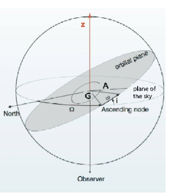
Figure 3: The orbital plane and orbit of component A around the centre of mass G. $z$ is the coordinate along the line of sight, pointing away from the observer. The plane of the sky is tangent to the celestial sphere and perpendicular to the line of sight.

3.2 Roche lobe

The concept of the Roche lobe is central while dealing with binary stars. Let us consider a circular binary and a test particle corotating with this binary, such as a mass element on the surface of a star rotating synchronously with the orbital realiasvolution. The Roche lobe corresponds to the critical equipotential (in the corotating reference frame) surface around the two binary-system components which contains the inner Lagrangian point. At this point the net force acting on the corotating test mass vanishes (the net force is the vector addition of the two gravitational forces and of the centrifugal force arising in a non-inertial reference frame rotating uniformly with the binary). If the star swells so as to fill its Roche lobe, matter will flow through the inner Lagrangian point onto the companion. The radius of a sphere with the same radius as the Roche lobe around star A may be expressed by (Eggleton, 1983):

$$R_{R,A}/a=\frac{0.49\;q^{-2/3}}{0.6\;q^{-2/3}+\ln(1+q^{-1/3})},$$ (7)

where $q=M_{B}/M_{A}$ is the mass ratio. In the case of a star losing mass (like an AGB star), the extra-force responsible for the ejection of the wind must be included in the effective potential. It distorts the shape of the equipotentials and reduces the size of the Roche lobe around the mass-losing star (Schuerman, 1972). To take this effect into account, a generalisation of Eggleton’s formula is necessary (Dermine and Jorissen, 2008). This reasoning is strictly applicable only to circular systems, but is often employed as an useful approximation also in the case of non-zero eccentricity. A more detailed discussion of the concept of Roche lobe is given by, e.g., Shore (1994) or Jorissen (2003a).

4 Spectroscopy

4.1 The method

Spectroscopic detection of binaries relies on measuring the Doppler shifts of stellar spectral lines as the binary components orbit their centre of mass. Soon after the discovery of the first spectroscopic binaries in late nineteen century (Vogel, 1890; Pickering, 1890) this became the preferred detection method as it is robust and through relatively simple means it gives access to important physical parameters. Time-dependent spectroscopy allows direct determination of $P,T_{0},e,$ and $\omega$ – period is the easiest to constrain, the other parameters require more detailed knowledge of the shape of the radial-velocity curve. Radial velocities give no handle on $\Omega$, but convey entangled information on $a$ and $i$. Joined with Kepler’s third law, this leads to partial, but very much sought after, knowledge concerning the component masses (see Sect. 4.3 and Table 5 in Sect. 8).

The expression for the radial-velocity of star A is

$$V_{r}({\rm A})=V_{r}({\rm G})\;+\;{\rm d}z({\rm A})/{\rm d}t=V_{r}\left({\rm G})\;+\;K_{A}\left(e\cos\omega+\cos(\omega+\nu(t)\right)\right),$$ (8)

where $V_{r}(\mathrm{G})$ is the radial velocity of the centre of mass of the system, $z$ is the spatial coordinate along the line of sight (Fig. 3), $\nu$ is the true anomaly (angle between periastron and the true position of the star on its orbit), and (e.g., Smart, 1977)

$$K_{A} = \frac{2\pi}{P}\frac{a_{A}\sin i}{(1-e^{2})^{1/2}}$$

$$= 212.9\;\left[\frac{M_{A}({\rm M}_{\odot})}{P({\rm d})}\right]^{1/3}\frac{q}{(1+q)^{2/3}}\;\;\frac{\sin i}{(1-e^{2})^{1/2}}\;\;{\rm km\;s}^{-1}$$

$$= 212.9\;\left[\frac{M_{B}({\rm M}_{\odot})}{P({\rm d})}\right]^{1/3}\left(\frac{q}{1+q}\right)^{2/3}\frac{\sin i}{(1-e^{2})^{1/2}}\;\;{\rm km\;s}^{-1}$$

is the semi-amplitude of the radial-velocity curve of component A, with $q=M_{B}/M_{A}$. To fix the ideas, the semi-amplitude $K_{A}$ associated with companions of various masses and orbital periods is given in Table 1, for a 3 M_⊙ primary star in a circular orbit with $i=90^{\circ}$.

Table 1: The semi-amplitude $K_{A}$ (in km s^-1) associated with companions of various masses and orbital periods, for a 3 M_⊙ primary star in a circular orbit with $i=90^{\circ}$.

$M_{B}$ (M⊙)    $P=$	3 d	30 d	1 yr	3 yr
3	134	62	27	19
1	59	27	12	8
0.6	38	17	8	5
0.08	6	3	1	0.8

4.2 One-dimensional observation: the uncertainty introduced by the inclination

The first difficulty facing spectroscopic-binary detection comes from the fact that the radial velocity is a one-dimensional measurement (along the line of sight), which implies that the knowledge of the orbit can only be partial. In particular, what is known is the projected orbit on the plane of the sky, implying a degeneracy between $i$ and $a_{A}$, since only the combination $a_{A}\sin i$ may be extracted from $K_{A}$. The same expression holds for component B if that component is visible (’SB2 systems’ standing for spectroscopic binaries with two observable spectra).

If the components of a binary are of approximately equal luminosities, the spectrum will appear as ’composite’ (as further discussed in Sect. 7.3), and a radial-velocity curve (Eq. 8) will be available for both components. Since $a_{A}M_{A}=a_{B}M_{B}$ from the definition of the centre of mass, the mass ratio $q=M_{B}/M_{A}$ may be derived from $K_{A}/K_{B}$ (see Eq. 4.1). Then, $K_{A}+K_{B}$ joined with Kepler’s third law

$$a^{3}/P^{2}=G\;(M_{A}+M_{B})/4\pi^{2},$$ (10)

where $a=a_{A}+a_{B}$ is the semi-major axis of the relative orbit, gives access to $(M_{A}+M_{B})\sin^{3}i$ (since only $a\sin i$ – not $a$ – may be extracted from $K_{A}+K_{B}$). Combining the mass ratio and sum (multiplied by $\sin^{3}i$) then yields $M_{A}\sin^{3}i$ and $M_{B}\sin^{3}i$ for the case of SB2 binaries. A summary of what may be known about the masses for spectroscopic binaries is provided by Table 5 in Sect. 8.

If there is an independent way to derive the orbital inclination $i$ (the system is visual, astrometric or eclipsing; in the latter case $i$ is close to 90^∘), then (and only then) may the individual masses be derived (see Table 5). A textbook case (among many others; see the review in Andersen, 1991) is provided by the S star HD 35155 : this star is a spectroscopic binary with only one spectrum visible in the optical region (Udry et al., 1998), but an International Ultraviolet Explorer (IUE) spectrum reveals ultraviolet emission lines tied to the companion (Ake et al., 1991; Jorissen et al., 1992a), which thus gives access to the mass ratio. Eclipses have been observed in IUE spectra and optical photometry (Jorissen et al., 1992a, 1996), which implies an inclination close to 90^∘. With all these data at hand, the masses inferred for the giant and its companion are 1.3 – 1.8 M_⊙ and 0.45 – 0.6 M_⊙, respectively (Jorissen et al., 1992a).

If one is only interested in the distribution of the masses (rather than in the masses of individual objects) for a sample of SB2 binaries with their orbital planes inclined randomly on the sky, then statistical techniques may be used, as further discussed under the next item.

4.3 Only one spectrum is observable: the mass function

It must be stressed that the semi-major axis $a=a_{A}+a_{B}$ of the relative orbit cannot be derived if only one spectrum is observable (for instance in the case of a faint companion, on the lower main sequence or a WD). Hence Kepler’s third law, which involves $a$, is not applicable. Instead, for these binaries with only one observable spectrum (say A), only a quantity called the mass function and denoted $f(M)$, can be derived:

$$f(M)\;\;=\;\;\frac{(M_{B}\sin i)^{3}}{(M_{A}+M_{B})^{2}} = \frac{\;K_{A}^{3}\;P\;}{2\pi\,G}\;\;(1-e^{2})^{3/2}$$ (11)

$$= 1.036\times 10^{-7}\;\,K_{A}^{3}({\rm km\;s}^{-1})\;P({\rm d})\;(1-e^{2})^{3/2}\;{\rm M}_{\odot}$$ (12)

Still, there is a way to get better constraints on the masses if specific conditions are met, namely $M_{B}<<M_{A}$ (exoplanet companion) with $M_{A}$ known from the mass-luminosity relationship for main-sequence stars (if applicable). In those circumstances, Jorissen et al. (2001) have shown that, for a sample of stars, it is possible to extract the distribution of $M_{B}$ from the observed distribution $\Phi(Y)$ of $Y(M_{B})\equiv M_{B}\sin i$. This follows from

$$\textrm{\phantom{blabla (since $M_{B}<<M_{A}$).}}f(M)\approx\frac{M_{B}^{3}\;\sin^{3}i}{M_{A}^{2}}\textrm{\phantom{blabla} (since $M_{B}<<M_{A}$).}$$

As $M_{A}$ is known, $Y(M_{B})$ may be derived from $Y(M_{B})=f(M)^{1/3}M_{A}^{2/3}$.

In the more general case of a stellar rather than planetary companion, and with $M_{A}$ known (as above), the distribution of $Q\equiv q\;(1+q)^{-2/3}$, where $q=M_{B}/M_{A}$, may be obtained rather than that of $M_{B}$ (Cerf and Boffin, 1994). Indeed, we have $f(M)=M_{A}\;q^{3}\;(1+q)^{-2}\sin^{3}i=M_{A}\;Q^{3}\sin^{3}i$. Hence, $Y(Q)\equiv Q\sin i=f(M)^{1/3}M_{A}^{-1/3}$ is available from the observations.

Then, the sought distributions $\Psi(M_{B})$ or $\Psi(Q)$ obey the relation:

$$\Phi(Y)=\int_{0}^{\infty}\Psi(M_{B})\;\Pi(Y|M_{B})\;{\rm d}M_{B}\quad{\rm or}\quad\Phi(Y)=\int_{0}^{\infty}\Psi(Q)\;\Pi(Y|Q)\;{\rm d}Q.$$

The kernel $\Pi(Y|M_{B})$ corresponds to the conditional probability of observing the value $Y$ given $M_{B}$. Under the assumption that the orbits are oriented at random in space, the inclination angle $i$ distributes as $\sin i:\Pi(i)\;{\rm d}i=\sin i\;{\rm d}i$ and the expression for the kernel is obtained from:

$$\Pi(M_{B}\sin i)M_{B}\cos i\;{\rm d}i=\sin i\;{\rm d}i.$$

Eliminating the inclination in the above relation yields

$$\Pi(Y|M_{B})=\frac{Y}{M_{B}}\frac{1}{(M_{B}^{2}-Y^{2})^{1/2}}\quad\quad\mbox{\rm with}\quad Y\leq M_{B},$$ (13)

and

$$\Phi(Y)=Y\int_{Y}^{\infty}\Psi(M_{B})\;\frac{1}{M_{B}(M_{B}^{2}-Y^{2})^{1/2}}\;{\rm d}M_{B}.$$ (14)

This integral equation must be solved for $\Psi(M_{B})$. It can be reduced to Abel’s integral equation by the substitutions (Chandrasekhar and Münch, 1950)

$$Y^{2}=1/\eta\hskip 6.0pt{\rm and}\hskip 6.0ptM_{B}^{2}=1/t.$$ (15)

With these substitutions, Eq.(14) becomes

$$\phi(\eta)=\int_{0}^{\eta}\frac{\psi(t)}{(\eta-t)^{1/2}}\;{\rm d}t,$$ (16)

where

$$\phi(\eta)\equiv\Phi(\frac{1}{\sqrt{\eta}})\hskip 6.0pt{\rm and}\hskip 6.0pt\psi(t)\equiv\frac{1}{2\;\sqrt{t}}\Psi(\frac{1}{\sqrt{t}}).$$ (17)

The formal solution of Abel’s equation (Eq. 16) is given by

$$\psi(t)=\frac{1}{\pi}\int_{0}^{t}\frac{\partial\phi}{\partial\eta}\frac{1}{(t-\eta)^{1/2}}\;{\rm d}\eta+\frac{1}{\pi}\frac{\phi(0)}{\sqrt{t}},$$ (18)

where $\phi(0)={\rm lim}_{Y\rightarrow\infty}\Phi(Y)=0$.

It is difficult to implement numerically, since it requires the differentiation of the observed frequency distribution $\Phi(Y)$. Unless the observations are of high precision, it is well known that this process can lead to misleading results. Two approaches are possible to overcome that difficulty:

• The observed frequency distribution is smoothed in an optimal way before being used in Eq. 18 (Silverman, 1986). The solution $\Psi(t)$ is then computed numerically using standard differentiation and integration schemes.

• The Lucy-Richardson inversion algorithm is applied to Abel’s integral equation (Cerf and Boffin, 1994; Lucy, 1974; Richardson, 1972).

Both methods have been used by Jorissen et al. (2001) to derive the distribution of exoplanet masses.

Figure 4: AAVSO light curve (filled dots) for the Mira variable R CMi during three successive cycles, compared to its radial-velocity curve (solid line and open dots, from Udry et al. (1998)). Radial-velocity measurements were not necessarily obtained at the indicated dates, as they were all folded onto the radial-velocity solution. Note that the light- and velocity-curves are phase-shifted: maximum light occurs when the velocity curve crosses the centre-of-mass velocity (represented by the horizontal dashed line). (From (Jorissen, 2003a))

4.4 Intrinsic velocity variations

4.4.1 Pseudo-orbital variations and Roche lobe radius

Figure 5: The radial-velocity curve of the RV Tau variable IRAS 08544-4431: the variations with a large amplitude are caused by the orbital motion, whereas the small-amplitude variations are caused by the RV Tau-like pulsations with period 90 d, as shown on the bottom panel, displaying the residuals with respect to the orbital solution. (From (Maas et al., 2003))

The pulsation of the atmosphere of Mira, Cepheid or RV Tau variables causes intrinsic velocity variations and makes binary detection using radial velocities difficult or even impossible. Often the radial-velocity variations associated with the pulsations are with the same period as the photometric variations (although they are phase-shifted), so that the intrinsic nature of these radial-velocity variations is very clear. A very spectacular example is provided by the comparison of the light curve of the 337 d Mira variable R CMi with its radial-velocity curve, as shown on Fig. 4. The radial-velocity semi-amplitude is as large as 8 km s^-1. Clearly, in such a case, a companion could only be detected if it would yield orbital variations of at least the same order (compare with the data of Table 1 to see which kind of companions would be detectable).

Hinkle et al. (1997) have shown that the radial-velocity semi-amplitude associated with Mira and semi-regular pulsators correlates well with the visual amplitude and with the pulsation period, reaching 15 km s^-1 in the most extreme cases.

The binary post-AGB star IRAS 08544-4431, hosting a RV Tau variable (a class of luminous variables in the Cepheid instability strip, characterized by alternating deep and shallow minima), is a rare case where intrinsic and orbital radial-velocity variations are superimposed (Maas et al. 2003 (Maas et al., 2003) present in fact quite a number of similar cases). Here the orbital period is 499 d and the orbital semi-amplitude is 8 km s^-1, to be compared to 4 km s^-1 for the pulsations of period 90 d (Fig. 5). Hence the two kinds of variations may be separated, but at the expense of a dense observational coverage.

Figure 6: Left panel: The radial-velocity curve of the 222 d-period Mira variable S UMa. A solution with a period $P=576$ d and an eccentricity of 0.29 provides a good match to all the data points but the last two. Since the 1/576 d^-1 frequency is close to the 1/222.0 - 1/365.25 alias of the 1-yr frequency and of the pulsation frequency, the intrinsic origin of the radial-velocity variations becomes the best explanation. From (Famaey et al., 2008). Right panel: The radial-velocity data of S UMa phased with the 222 d pulsation period. The solid line is an (unsatisfactory) keplerian solution of eccentricity 0.29.

Sometimes, however, the situation is not as clear as for the two cases discussed above. The 225.9 d Mira variable S UMa exhibits radial velocity variations that could at first be interpreted as orbital motion with an apparent period of 576 d and an eccentricity of 0.29 (Udry et al., 1998), based on a rather scarcely sampled data set (Fig. 6). However, the last two data points deviate markedly from the solution based on earlier data points, casting doubts on that solution. A period analysis of this data set (Famaey et al., 2008) reveals that the 576 d period is probably an alias of the pulsation period (present in the radial-velocity data as 222.0 d) and of 1 yr (1/222.0 - 1/365.25 = 1/566.0), thus strongly reinforcing the suspicion that the radial-velocity variations have an intrinsic origin.

In any case, periods as short as a few hundred days can in no way be associated with an orbital motion involving a star as large as a Mira, since the Mira would then fill its Roche lobe, and the system would exhibit strong signatures of mass transfer (like for instance an X-ray flux, or strong emission lines). To hold within a binary system, the radius $R$ of a Mira variable derived from the relationships (Van Leeuwen et al., 1997)

$$\log R_{\rm Mira}=(\log P+0.9\log M+2.07)/1.9 \,{\rm fundamental\;mode,}$$

$$\log R_{\rm Mira}=(\log P+0.5\log M+1.40)/1.5 \,{\rm first\;overtone\;mode,}$$

where $P$ is expressed in days, and $R$ and $M$ in solar units, must be smaller than the critical Roche lobe radius $R_{R}$ expressed by Eq. 7 (Eggleton, 1983; Dermine and Jorissen, 2008). The orbital period for which a Mira of a given pulsation period (in either the fundamental or first overtone mode) fills its Roche lobe is displayed in Figure 7. It is derived from the above formulae (7) and (4.4.1), and from Kepler’s third law (assuming typical masses for the Mira star and its companion, as indicated on the figure).

Figure 7: Bottom panel: Orbital periods versus pulsation periods for Miras in semi-detached systems, derived from the period–radius relations (Eq. 4.4.1) for the fundamental and first overtone modes. Detached systems are located above the corresponding lines. The filled circles labeled M0 and M7 indicate the critical periods corresponding to the median radii of non-Mira M0 and M7 giants (Dumm and Schild, 1998), respectively (adopting masses of 1.0 and 0.75 M_⊙ for the giant and its companion, respectively). Top panel: Orbital radial-velocity semi-amplitude versus pulsation periods (thick lines: fundamental mode; thin lines: first overtone) for Miras in circular semi-detached systems with $\sin i=1$ (where $i$ is the orbital inclination). Binary systems with larger semi-amplitudes would involve Roche-lobe-filling AGB stars. (From (Jorissen, 2003a))

The orbital periods allowed by this criterion are quite long (more than 1000 d), and are always much longer than the pulsation periods. The corresponding radial-velocity semi-amplitudes $K$ (Fig. 7) may be computed from Eq. 4.1. This quantity must be compared with the intrinsic radial-velocity variations of Mira variables (due to pulsations) which can be as high as 15 km s^-1 (Hinkle et al., 1997). The detection of spectroscopic binaries among Mira variables thus appears to be almost impossible.

4.4.2 Wood’s sequence D and long secondary periods

Variable stars with ’long secondary periods’ (LSP, characterized by periods between 200 and 4000 days, i.e., a factor 5 to 15 longer than the primary period) and with $V$-band amplitudes up to 1 mag have been known for decades (Payne-Gaposchkin, 1954; Houk, 1963), but the interest for it has been renewed since Wood (Wood et al., 1999; Wood, 2000) showed that these secondary periods follow a period-luminosity (PL) relation (the so-called ’sequence D’) in the PL diagram of long-period variables (LPVs) in the LMC. Besides the expected sequence corresponding to the fundamental pulsation mode of Miras (the so-called ’sequence C’) and its higher harmonics (sequences A, A’ and B, mainly populated by semi-regular variables), a sequence very clearly appeared at longer periods (the so-called ’sequence D’; Fig. 8), involving about 25% of the LPVs in the LMC. Various hypotheses have been proposed to explain the origin of the LSP variability: rotation of a spotted star, episodic dust ejection or obscuration, radial or non-radial pulsations, stellar or substellar companions. Wood et al. (1999) suggested that stars on sequence D are components of semi-detached binary systems. But is it possible that 25% of all the LPVs in the LMC are member of binary systems, let alone semi-detached systems?

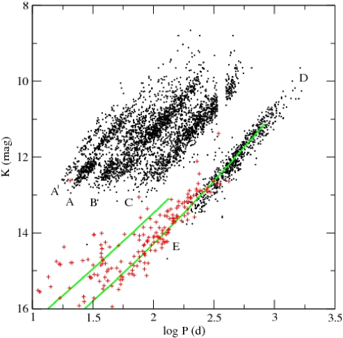
Figure 8: Period-luminosity relations for red giant pulsators discovered by the MACHO project in the Large Magellanic Cloud. Ellipsoidal and contact eclipsing binaries are shown as plus signs. The solid lines show the critical orbital periods for systems of unit mass ratio filling their Roche lobe, with primary masses of 0.85 and 2.5 M_⊙. (From (Derekas et al., 2006))

Derekas et al. (2006) and Soszyński et al. (2004) noticed that the so-called ’sequence E’, containing eclipsing and ellipsoidal binaries, is the extension of sequence D for fainter (i.e. non LPV) stars. Soszyński (2007) obtained another clear result calling for the role of binarity in the LSP phenomenon: by considering the quantity $1.3R_{M}-B_{M}$ (where $R_{M}$ and $B_{M}$ are the MACHO magnitudes in the red and blue bands, respectively), the LSP phenomenon should disappear since Derekas et al. (2006) found that LSP stars have a $B_{M}/R_{M}$ amplitude ratio of 1.3 on average, as compared to 1.1 for ellipsoidal variability, which should be grey. Soszyński (2007) found that in 5% of the stars belonging to sequence D, a double-humped structure with a period equal to the LSP one is observable in the $1.3R_{M}-B_{M}$ residual lightcurve, but with a slight phase lag with respect to the LSP lightcurve. This finding gives credit to the binary hypothesis, and the phase shift even hints at dust obscuration as being responsible for the double-humped lightcurve, since hydrodynamical simulations of the mass transfer involving a mass-losing AGB star reveals that the accretion column forms a spiral arm behind the companion (Fig. 9; Theuns and Jorissen, 1993; Theuns et al., 1996; Mastrodemos and Morris, 1998; Nagae et al., 2004; Jahanara et al., 2005). Therefore, the eclipse of the star by this matter trailing behind the companion occurs slightly before the geometric conjunction.

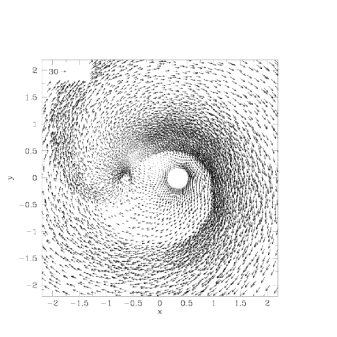
Figure 9: The structure of the flow (represented by its velocity field) from a mass-losing AGB star (located at $x=0.33,y=0$) around the accreting star (located at $x=-0.66,y=0$) in a frame rotating with the system. The double-spiral structure is clearly visible in this simulation of an adiabatic flow. (From (Theuns et al., 1996))

This will be discussed further below in Sect. 5.3, where we will show that such dust obscuration events are rather common among binaries involving mass-losing giants. The dust cloud present in the LSP stars is not very conspicuous, though, since mid-infrared colors of LSPs and non-LSPs are similar (Olivier and Wood, 2003; Wood et al., 2004) and there are no LSPs showing the large [60]-[25] $\mu$m IRAS excesses exhibited by some R Coronae Borealis stars, a class of stars known for forming dust in large quantities.

Another piece of evidence in favour of binarity was presented by Derekas et al. (2006), Soszyński et al. (2004), Soszyński (2007) and Jorissen et al. (2008) who showed that Wood’s sequence D closely matches the sequence expected for binary stars involving giant stars filling their Roche lobe. This is clearly illustrated by the solid lines in Fig. 8 and by Fig. 10, which is a diagram orbital-period – luminosity for the exhaustive sample of spectroscopic binary M giants from Jorissen et al. (2008). The ordinate axis of Fig. 10 corresponds to the $K$ magnitude that these M giants would have if they were at the distance of the LMC, i.e., $K({\rm LMC})=M_{K}+18.50$, where the McNamara et al. (2007) LMC distance modulus has been adopted, and the absolute $K$ magnitude is derived from the 2MASS value combined with the distance from the maximum-likelihood estimator of Famaey et al. (2005). It is very clear that Wood’s sequence D does indeed come close to the upper envelope of the region occupied by the galactic binary M giants, which is defined by the condition that they hold within their Roche lobe.

If Wood’s sequence D is indeed related to LPVs filling their Roche lobe, the remaining question is: how come that there are so many? Soszyński (2007) suggests that variability along sequence D originates in giants with substellar companions, the latter being supposedly much more numerous than the 15% of spectroscopic binaries (not even restricting to semi-detached systems) observed among M giants (Frankowski et al., 2008). Although the mass functions of the orbital solutions obtained by Wood et al. (2004) and Hinkle et al. (2002) are indeed compatible with substellar companions, the eccentricities and longitudes of periastron derived for 5 among the 6 orbits presented by (Hinkle et al., 2002) are surprisingly similar and may cast doubts on the orbital origin of the observed variations.

Figure 10: The orbital-period as a function of (absolute) $K$ magnitude for galactic M giants in binary systems. The ordinate axis corresponds to the $K$ magnitude that the M giants would have if they were put at the distance of the LMC (see text). The dashed line labelled ’D’ corresponds to Wood’s sequence of long secondary periods. The solid and dotted lines correspond to the limit on the orbital period imposed by the Roche lobe radius (for $M_{1}=1.3$ M_⊙ and $M_{2}=0.6$ M_⊙), for stellar radii comprised between 40 and 120 R_⊙. (From (Jorissen et al., 2008)).

5 Photometry

As stated in the previous section on spectroscopic binaries, not many spectroscopic binaries are known among Mira variables, because the orbital radial-velocity semi-amplitude $K_{\rm orb}$ corresponding to a long-period binary is generally smaller than $K_{\rm puls}$. Other methods must thus be used to detect binaries involving Mira variables! Fortunately, there are specific methods using photometry to do so.

5.1 Miras with flat-bottom light curves

Miras exhibiting a light curve with a flat bottom and a small-amplitude, despite their Mira-like period, are good candidates for being binaries with a faint companion, which dominates the system light around minimum light and is responsible for the flat bottom. A good example thereof is Z Tau ($P\sim 450$ d), whose AAVSO (see Sect. 9) light curve exhibits a flat bottom at $V=14$.

5.2 Ellipsoidal or eclipsing variables

Ellipsoidal variables are characterized by a light cycle which is exactly half the orbital period, caused by the tidal deformation of the star nearly filling its Roche lobe. The detection of ellipsoidal variations or of eclipses has often been the first evidence of binarity for many systems. It offers an easy way to infer the binary period (see Belczyński et al., 2000, for the case of symbiotic stars). Ellipsoidal variations should have the same amplitude in all photometric bands, as it is a purely geometrical effect (Hall, 1990).

5.3 Dust obscuration and circumbinary disks

Hydrodynamical simulations of a wind-driven accretion flow in binary systems (Theuns and Jorissen, 1993; Mastrodemos and Morris, 1998; Nagae et al., 2004; Jahanara et al., 2005; Edgar et al., 2008) predict the formation of a spiral pattern corresponding to the accretion wake bended by the Coriolis force (Fig. 9). This prediction has been nicely confirmed by the direct imaging in visible light of the proto-planetary nebula AFGL 3068, using the ACS camera on board the HST, which reveals a spiral pattern winding several times around the central star (Mauron and Huggins, 2006). Periodic obscuration of the central star by dust clumps trapped in the accretion structure – be it spiral wave, disk around the companion, or a circumbinary disk – seems common in binary systems involving a mass-losing giant star. This phenomenon very likely plays a role in the photometric variability observed in the following classes of stars:
Binary systems with evidence for dust obscuration Stellar class Examples References LSP Wood’s sequence D many (Soszyński, 2007) short $P_{\rm orb}$ Ba or S stars HD 35155, HD 46407, HD 121447 (Jorissen et al., 1992a, 1991, b) AGB C star V Hya (Knapp et al., 1999) Post-AGB HR 4049 (Waelkens et al., 1991a) Supergiants $\epsilon$ Aur (Lissauer et al., 1996)

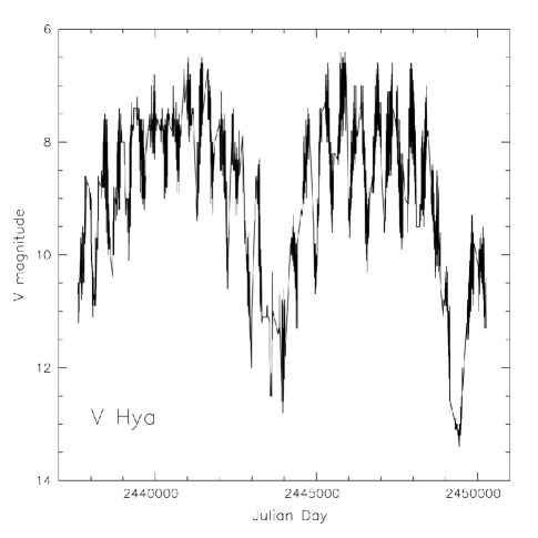
Figure 11: The $V$ band light curve of V Hya between October 1961 and July 1996 from the AAVSO archives. These data show a more or less regular variability with a period of 533 d and a peak-to-peak variation of 2 magnitudes at $V$, plus a longer-term variation with a period of about 6500 days (17–18 years) with deep minima (5 to 6 magnitudes). (From (Knapp et al., 1999))

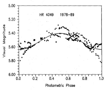
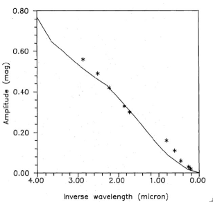
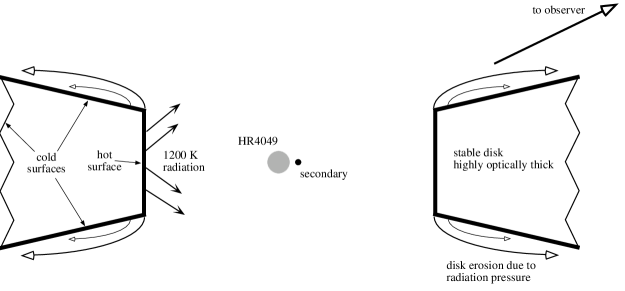
Figure 12: The $V$ light curve of the post-AGB star HR 4049 (upper left panel). The modulation is caused by the line of sight going through the dusty circumbinary disk once per orbit, according to the model depicted in the bottom panel. The upper right panel compares the amplitude of the variations in various photometric bands with the extinction law in the interstellar medium. (From (Waelkens et al., 1991a) and (Dominik et al., 2003))

The case is especially clear for the C star V Hya (Fig. 11). Quoting Knapp et al. (1999): The morphology of the 17 y variation resembles that of an eclipsing binary, but with an eclipse duration which is far longer than can be produced by a stellar companion and of an amplitude which shows that essentially the entire stellar photosphere is occulted. We suggest that the regular long-period dimming of V Hya is due to a thick dust cloud orbiting the star and attached to a binary companion. The orbital period is inferred from the light curve displayed on Fig. 11, and there is no spectroscopic confirmation so far (difficult because of the long period, hence small semi-amplitude!).

The 27-yr period observed in the F0 supergiant $\epsilon$ Aur (Lissauer et al., 1996) may be a similar case, with the long duration of the eclipse showing that the secondary cannot be a star but must be a large (510 AU) dark body, which observations strongly suggest is a dust disk orbiting a companion (Lissauer et al., 1996; Huang, 1965). Eclipses best explained by dust clouds attached to a binary companion are also seen in a small number of planetary nebula nuclei, e.g. in NGC 2346 (Costero et al., 1993). Finally, the prototypical post-AGB star HR 4049 exhibits eclipses by a dust disk, which has been imaged directly by VLTI (Fig. 12; Waelkens et al., 1991a; Dominik et al., 2003; Antoniucci et al., 2005). The geometry of the binary system (bottom panel of Fig. 12) is such that the line of sight goes through the circumbinary disk once per orbital cycle, thus the resulting light curve has only one minimum per cycle (upper left panel of Fig. 12) rather than two as in ellipsoidal variables. The color dependence of the amplitude of the variations is the same as the interstellar extinction law (upper right panel of Fig. 12), thus confirming that the optical variability is caused by scattering on dust grains of similar size as in the interstellar medium.

Such circumbinary disks are almost a defining property of binary post-AGB stars, since the presence of a 21 $\mu$m excess, caused by the presence of cold dust in a circumbinary disk extending far away from the heat source (the post-AGB star), may be used for identifying binary post-AGB stars (Van Winckel, 2003; de Ruyter et al., 2006; Van Winckel et al., 2006).

The M4III + A system SS Lep (= HD 41511) shares with post-AGB stars the presence of a circumbinary disk (Jura et al., 2001; Verhoelst et al., 2007), fed by non conservative RLOF. Using interferometry, Verhoelst et al. (2007) have indeed shown that the M giant fills its Roche lobe, and that the A type companion has a radius about 10 times larger than that expected for a main sequence star. It has very likely swollen as a result of accretion. The system HR 1129 (G2Ib + B7) shows as well an infrared signature of dust most likely associated with a circumbinary disk (Griffin et al., 2006a).

The lightcurves of the Ba star HD 46407 and the S star HD 35155 (see Fig. 13) are a bit more puzzling. Barium stars are post-mass-transfer objects with WD companions (McClure, 1984; Jorissen and Mayor, 1988; Böhm-Vitense et al., 2000) which are too faint to yield detectable eclipses in the visual. And yet, the reality of the eclipses in the short-period Ba star HD 46407 ($P=457$ d) cannot be doubted, since the eclipses have been observed during different cycles, though with variable depths and phase lags (Jorissen et al., 1991, 1992b). A very important clue as to the origin of these eclipses comes from the fact that the deepest eclipse (observed around JD $2\,447\,400$) has occurred just before an episode of secular obscuration (left panel of Fig. 14). The fact that the color dependency of the amplitude for both the eclipse and secular variations follows a $\lambda^{-4}$ law (right panel of Fig. 14), reminiscent of Rayleigh scattering, at least in the Strömgren $u$ and $v$ bands, is a further indication that the phenomenon is caused by (small) dust grains. In $b$ and $y$, it is closer to the ISM color absorption law. Despite the fact that barium stars host K giants which do not lose large amounts of mass, the secular obscuration event calls for the presence of recent dust in the system, rather than for the remnant of the spiral arm dating back to the epoch where the current WD companion was a mass-losing AGB star.

A similar eclipsing behaviour has been reported for the S star HD 35155 with 640 d period by (Jorissen et al., 1992a). Despite the fact that Adelman (2007) did not confirm the occurrence of the eclipse, the two IUE spectra of HD 35155 obtained by chance at the time of eclipse have the smallest flux among the 10 available IUE spectra, though neither the continuum nor the emission lines disappear completely (Ake et al., 1991; Jorissen et al., 1996).

HD 121447 is the coolest barium star (K7III) with the second shortest orbital period (186 d). Ellipsoidal variability was first suspected for this star (Jorissen et al., 1995), but the absence of synchronous rotation and a strong color dependence of the light curve (Adelman, 2007) do not support this conclusion, so that light variations caused by scattering on dust formed by the compression of the red-giant wind in the accretion process, becomes an attractive possibility.

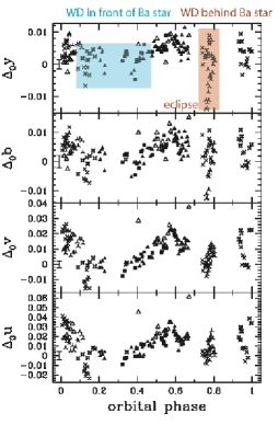
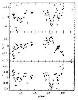
Figure 13: The light curves phased with the orbital period for the barium star HD 46407 (left panel; $P=457$ d) and the S star HD 35155 (right panel; $P=640$ d) which are among the systems with the shortest periods in these classes. Data for HD 46407 (Jorissen et al., 1991, 1992b) and HD 35155 (Jorissen et al., 1992a) in the Strömgren system from the Long-Term Photometry of Variables program (Manfroid et al., 1991). The small arrows in the right panel identify the phases corresponding to the eclipse (0.17) and transit (0.65) of the companion. HD 35155 exhibits as well intrinsic photometric variations.

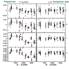
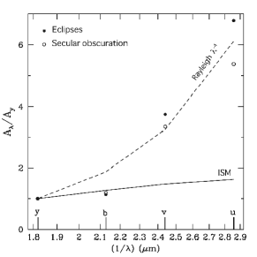
Figure 14: Left panel: The long-term light curve (in the Strömgrem bands $uvby$, from bottom to top) of HD 46407 with respect to the average of the comparison stars (left), and the difference between the two comparison stars (right). The solid line roughly illustrates the secular change in the average brightness. See Jorissen et al. (1992b) for details. Right panel: The amplitude of the secular and eclipse variations in the $u$, $v$ and $b$ bands normalized by the amplitude in the $y$ band, and comparison with the interstellar-medium extinction law and the Rayleigh $\lambda^{-4}$ law.

To summarize, disks (often circumbinary) are observed in many different classes of binary stars involving a mass-losing star, and seem to be very common in such circumstances. They play an important role in the evolution of such systems:
- they control the evolution of the eccentricity through tidal effects and angular momentum exchange with the orbit (Artymowicz et al., 1991);
- they trigger a dust/gas segregation, so that the abundance pattern observed at the surface of the post-AGB star is shaped by the condensation temperature of the various elements (Maas et al., 2005). It is believed that this physical segregation operates through re-accretion by the post-AGB star of gas depleted in refractory elements which stayed in the dust phase. It leads to very Fe-depleted post-AGB atmospheres (down to [Fe/H] $=-4.8$) (Waelkens et al., 1991b). Intriguingly, a similar scenario has recently been proposed (Venn and Lambert, 2008) as the possible cause of the ultra low metallicities observed in several stars from the Hamburg/ESO survey (Reimers and Wisotzki, 1997), like the record holder HE 1327-2326 with [Fe/H] $=-5.6$ (Venn and Lambert, 2008; Frebel et al., 2005). This scenario would require these stars to be binaries. There is no definite evidence thereof so far, but the available radial-velocity data is not necessarily conclusive (Venn and Lambert, 2008).

6 Astrometry

6.1 The basics

Very long-period systems are hard to detect with spectroscopy or photometry. This is where astrometry comes to rescue. Astrometric binaries differ from the more traditional visual binaries in the sense that for visual binaries, both components are observed so that it is the relative orbital motion (of one component with respect to the other) which is readily detected. For astrometric binaries instead, it is the absolute (non-linear) motion of one component on the sky which is detected. Space astrometry, which started with the Hipparcos satellite (ESA, 1997) launched in 1989, has reached the milliarcsecond (mas) accuracy level for stars down to about $V=10$, and the coming Gaia satellite (to be launched in 2011) should improve this accuracy by a factor of 100. Many achievements have already been made in the field of binary stars by Hipparcos, as reviewed by Perryman (2008), and many more must be expected from Gaia. We will discuss just a few here, illustrating the potential of astrometry in the discovery of specific kinds of binaries (A very extensive review of this potential is presented in Perryman, 2008). For instance, since astrometric methods are independent of spectral types (as opposed to spectroscopic methods, since the detection of spectroscopic binaries is dependent upon the possibillity to follow accurately the variations of the position of spectral lines), astrometry offers a way to derive unbiased frequencies of binaries of different spectral types (Table 3; Frankowski et al., 2007). Substellar companions may also be detected thanks to astrometry, if accurate enough (Kaplan and Makarov, 2003; Makarov, 2004; Makarov and Kaplan, 2005). Astrometry offers as well good prospects to detect binaries involving Mira variables (which are especially difficult to find with spectroscopy), provided however that spots or an inhomogeneous surface brightness or asymmetries in the shape of the stellar disk of these very extended stars do not cause variations of the position of the photocentre that confuse the parallactic and orbital motion (Bastian and Hefele, 2005; Eriksson and Lindegren, 2007).

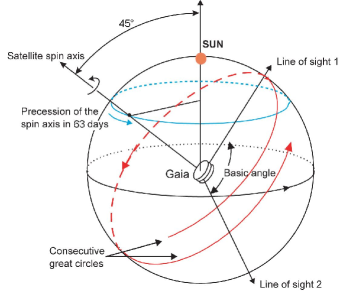
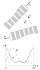
Figure 15: Left panel: The scanning law of Gaia. (From the ESA-Gaia web site) Right panel: The modulating grid in the Hipparcos focal plane (top), for two different scanning directions A and B, producing the modulated signals displayed on the bottom panel. The phase $p$ for the source $S$ is measured differentially with respect to that of the reference point $R$, modulo the grid step. In reality, the grid extends over the images of $S$ and $R$ in the focal plane, although this was not displayed for clarity. (From (Quist and Lindegren, 1999))

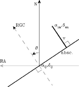
Figure 16: Definition of the abscissa offset $v$ for a predicted position $(\alpha_{m},\delta_{m})$, with respect to the observed position somewhere along the thick line perpendicular to the reference great circle labeled ’RGC’. Remember that the measurement is one-dimensional. (From (van Leeuwen and Evans, 1998))

The principle of the astrometric measurement by Hipparcos and Gaia needs to be explained first. In order to achieve a good accuracy overall on the celestial sphere, Hipparcos had two fields of view, 0.8 degree square each, widely separated on the sky (by about 58 degrees of arc) and superimposed on the detector. In the case of Gaia, the numbers will be 0.37 degree square and 106.5 degrees, respectively (left panel of Fig. 15). Since the satellite is spinning, this signal from stars crossing the instrument fields of view is modulated by a one-dimensional grid in the focal surface (right panel of Fig. 15). As the satellite scanned the sky in a complex series of precessing great circles, maintaining a constant inclination to the Sun’s direction, a continuous pattern of one-dimensional measurements was built up. In order words, it is the ’abscissa’ along the great circle which is being measured, the position of the star along the perpendicular to the reference great circle being unknown. These one-dimensional abscissa measurements are then confronted to the expected positions of the star on the sky as a function of time, for a given reference position, parallax and proper motion for that star. The difference between these one-dimensional positions is called ’abscissa residual’, and is noted $v$ on Fig. 16 (van Leeuwen and Evans, 1998). These abscissa residuals are then combined with the variance-covariance matrix of the observational errors to yield a $\chi^{2}$ value characterizing the quality of the solution (van Leeuwen and Evans, 1998; Pourbaix and Jorissen, 2000).

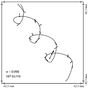
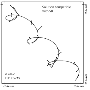
Figure 17: Left panel: A solution fitting the astrometric motion of HIP 85749 with a quasi-parabolic orbit ($e=0.998$) aligned with the line of sight. Right panel: The orbital solution with $e=0.2$, consistent with the spectroscopic orbital elements. Both solutions have similar goodness-of-fit values. The small line segments connect the predicted position with the observed great-circle abscissa (see Fig. 15). (From (Pourbaix, 2002))

Right away, two difficulties become apparent in the context of binary stars:
(i) It is the position of the photocentre of the system which is measured, reducing to the position of the brightest component if the difference in brightness is large. It may be shown (Binnendijk, 1960) that the relation between the semi-major axis $a_{0}$ of the orbit of the photocentre around the centre-of-mass and semi-major axis $a$ of the relative orbit writes

$$a_{0}=a(\kappa-\beta),$$ (20)

where $\kappa=M_{2}/(M_{1}+M_{2})$ and $\beta=1/(1+10^{0.4\Delta m})$, where $\Delta m=m_{2}-m_{1}$, so that when component 2 is much fainter than component 1 (i.e., $\Delta m\rightarrow\infty$), $\beta=0$ and $a_{0}=a\kappa$ is then the semi-major axis of the orbit of component 1 around the centre-of-mass. Therefore the access to the masses is not straightforward from astrometric orbits. A summary of what may be known about the masses for the various kinds of binaries (and combinations thereof) is listed in Table 5 in Sect. 8.
(ii) The one-dimensional nature of the astrometric (Hipparcos or Gaia) measurement imposes further limitations on the derivability of the orbital elements. As discussed by Pourbaix (2002), two-dimensional observations make it possible to draw an orbit projected on the plane of the sky, and to derive the areal constant $\Gamma^{\prime}$ of Kepler’s second law corresponding to the motion of the star on that projected orbit. Since the law of areas holds in both the true and projected orbits, one may write $\Gamma^{\prime}=\Gamma\cos i$, where $\Gamma$ is the areal constant in the true orbit, which is related to the orbital elements through the relation $\Gamma=a^{2}(1-e^{2})^{1/2}2\pi/P$ and may thus be derived from these. The ratio $\Gamma^{\prime}/\Gamma$ then yields the inclination. With one-dimensional measurements, $\Gamma^{\prime}$, and therefore $i$, cannot be derived accurately. In those circumstances, the derived $\Gamma^{\prime}$ value is often close to 0, so that $i$ close to 90^∘ follows (edge-on orbits). To accomodate the limited arc span on the sky with this spurious edge-on orbit, there is no other possibility than an eccentricity very close to unity (quasi-parabolic orbit), a very large semi-major axis and a longitude of periastron close to $90^{\circ}$ (apsidal line aligned with the line of sight). This is illustrated in Fig. 17, which compares two possible solutions (having similar goodness-of-fit values) fitting the astrometric motion of HIP 85749. The left panel is a solution with a quasi-parabolic orbit ($e=0.998$), an inclination close to $90^{\circ}$ and a large semi-major axis, whereas the right panel displays the solution with $e=0.2$ consistent with the spectroscopic orbital elements.

Even when spectroscopic orbital elements are known, spurious astrometric orbits with an inclination close to $90^{\circ}$ may still arise, as found by Jancart et al. (2005, see Fig. 18). These authors have designed statistical tests to identify those spurious solutions. A more detailed description of these astrometric methods to detect binaries is given in the next section.

Figure 18: Solid line: The distribution of orbital inclinations (from the Thiele-Innes set of orbital elements) for the 1385 orbits from the Ninth Catalogue of Spectroscopic Binary Orbits (Pourbaix et al., 2004a) with an Hipparcos entry. Many of those astrometric orbital solutions are spurious, with inclinations close to $90^{\circ}$. Dashed line: The same for the solutions passing all consistency tests defined by Jancart et al. (2005).

6.2 Detecting binaries from astrometric data

A tailored reprocessing of the Hipparcos (and in the future, Gaia) Intermediate Astrometric Data (hereafter IAD; van Leeuwen and Evans, 1998) makes it possible to look for orbital signatures in the astrometric motion, following the method outlined in (Pourbaix and Jorissen, 2000), (Pourbaix and Boffin, 2003), (Pourbaix, 2004) and applied to barium stars in (Jorissen et al., 2005) and (Jorissen et al., 2004).

The basic idea is to quantify the likelihood of the fit of the Hipparcos IAD with an orbital model. For that purpose, Pourbaix and Arenou (2001) (see also Jancart et al., 2005) introduced several statistical indicators to decide whether to keep or to discard an orbital solution. The relevant criteria are as follows (we keep the notation from (Jancart et al., 2005)):

• The addition of 4 supplementary parameters (the four Thiele-Innes orbital constants; see Eq. 1 and Sect. 3.1) describing the orbital motion should result in a statistically significant decrease of the $\chi^{2}$ for the fit of the $N$ IAD with an orbital model with 9 free parameters ($\chi^{2}_{T}$), as compared to a fit with a single-star solution with 5 free parameters ($\chi^{2}_{S}$, the 5 parameters being the the positions $\alpha$, $\delta$, the proper motions $\mu_{\alpha}$, $\mu_{\delta}$ and the parallax $\varpi$). This criterion is expressed by an $F$-test:

  $$Pr_{2}=Pr[F(4,N-9)>\hat{F}],$$ (21)

  where

  $$\hat{F}=\frac{N-9}{4}\;\;\frac{\chi^{2}_{S}-\chi^{2}_{T}}{\chi^{2}_{T}}.$$ (22)

  $Pr_{2}$ is thus the first kind risk associated with the rejection of the null hypothesis: “there is no orbital wobble present in the data”.

• Getting a substantial reduction of the $\chi^{2}$ with the Thiele-Innes model does not necessarily imply that the four Thiele-Innes constants $A,B,F,G$ are significantly different from 0. The first kind risk associated with the rejection of the null hypothesis “the orbital semi-major axis is equal to zero” may be expressed as

  $$Pr_{3}=Pr[\chi^{2}(4)>\chi^{2}_{ABFG}],$$ (23)

  where

  $$\chi^{2}_{ABFG}=\chi^{2}_{S}-\chi^{2}_{T}$$ (24)

  and $\chi^{2}(4)$ is a random variable following a $\chi^{2}$ distribution with four degrees of freedom.

• For the orbital solution to be a significant one, its parameters should not be strongly correlated with the other astrometric parameters (e.g., the proper motion). In other words, the covariance matrix ${\bf V}$ of the astrometric solution should be dominated by its diagonal terms, as measured by the efficiency $\epsilon$ of the matrix being close to 1 (Eichhorn, 1989). The efficiency is expressed by

  $$\epsilon=\sqrt[m]{\frac{\Pi_{k=1}^{m}\lambda_{k}}{\Pi_{k=1}^{m}{\bf V}_{kk}}},$$ (25)

  where $\lambda_{k}$ and ${\bf V}_{kk}$ are respectively the eigenvalues and the diagonal terms of the covariance matrix ${\bf V}$.

In other words, an orbital solution will be most significant if $Pr_{2}$ and $Pr_{3}$ are small and $\epsilon$ large. With the above notations, the requirement for a star to qualify as a binary was defined as

$$\alpha\equiv(Pr_{2}+Pr_{3})/\epsilon\leq 0.02,$$ (26)

where the threshold value of 0.02 has been chosen to minimize false detections, as derived from the application of the method to barium stars (see below and Jorissen et al., 2004).

Hipparcos data are, however, seldom precise enough to derive the orbital elements from scratch. Therefore, when a spectroscopic orbit is available beforehand, it is advantageous to import $e,P,T_{0}$ from the spectroscopic orbit and to derive the remaining astrometric elements (as done in Pourbaix and Jorissen, 2000; Jancart et al., 2005; Pourbaix and Boffin, 2003). The above scheme has been used by Jancart et al. (2005) to search for an orbital signature in the astrometric motion of binary systems belonging to the Ninth Catalogue of Orbits of Spectroscopic Binaries ($S\!_{B^{9}}$; Pourbaix et al., 2004a), and gives best results for systems with orbital periods in the range 100 – 3000 d and parallaxes in excess of 5 mas.

Figure 19: Left panel: Barium stars (previously known to be SBs) flagged as astrometric binaries by the algorithm are represented by black symbols. Arrows denote stars with only a lower limit available on the period. Right panel: Fraction of stars flagged as binaries (shaded histogram) compared to total number of stars, as a function of parallax. As expected, the detection rate becomes high for $\varpi>5$ mas. (From (Jorissen et al., 2004))

If a spectroscopic orbit is not available, trial $(e,P,T_{0})$ triplets scanning a regular grid (with $10\leq P(\rm d)\leq 5000$ imposed by the Hipparcos scanning law and the mission duration) may be used. The quality factor $\alpha$ (Eq. 26) is then computed for each trial $(e,P,T_{0})$ triplet, and if there exist triplets yielding $\alpha<0.02$, the star is flagged as a binary (In fact, scanning only $P$ with $e$ set to zero allows to save considerable computing time and would only miss very eccentric binaries). To test its success rate, this method has been applied by Jorissen et al. (2004) on a sample of barium stars. Barium stars constitute an ideal sample to test this algorithm, because they are all members of binary systems (Jorissen et al., 1998; McClure, 1983), with periods ranging from about 100 d to more than 6000 d. The catalogue of Lü et al. (1983) contains 163 bona fide barium stars with an Hipparcos entry (excluding the supergiants HD 65699 and HD 206778 = $\epsilon$ Peg). When $\varpi>5$ mas and $100<P(\rm d)<4000$, the (astrometric) binary detection rate is close to 100%, i.e., the astrometric method recovers all known spectroscopic binaries (Fig. 19). When considering the whole sample, the detection rate falls to 22% (= 36/163) because many barium stars have small parallaxes or very long periods. Astrometric orbits with $P>4000$ d ($>11$ yrs) can generally not be extracted from the Hipparcos IAD, which span only 3 yrs (see left panel of Fig. 19). Similarly, when $\varpi<5$ mas, as have most barium stars (right panel of Fig. 19), the Hipparcos IAD are not precise enough to extract the orbital motion.

When the orbit is not known beforehand, the method makes it even possible to find a good estimate for the orbital period, provided that the true period is not an integer fraction, or a multiple, of one year. Because parallactic motion has a 1-yr period, any orbital motion with a period corresponding to a (sub)multiple of 1 yr will not be easily disentangled from the parallactic motion. Therefore, for those periods, the parallax will be strongly correlated with the orbital parameters so that the efficiency $\epsilon$ (Eq. 25) will be small, causing $\alpha$ to be large (see Fig. 20).

Inspection of the run of $\alpha$ versus the trial periods $P$ clearly shows that $\alpha$ is minimum in the vicinity of the true (spectroscopic) orbital period (see left panel of Fig. 20). The period may thus be guessed by looking at the region where $\alpha$ is small. Conversely, for stars with no evidence of binarity from a radial-velocity monitoring, neither does astrometry find a period range where $\alpha$ becomes small (right panel of Fig. 21).

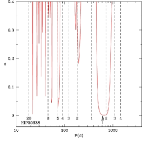
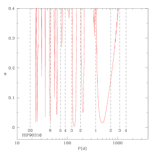
Figure 20: The $\alpha$ statistics (see Eq. 26) as a function of the trial orbital period (assuming $e=0$) for the $P=629$ d spectroscopic binary HIP 30338 (left panel). The vertical arrow indicates the spectroscopic period, which falls in the region of small $\alpha$. By comparison, a period of $\sim 500$ d may be inferred for HIP 90316 (right panel). The vertical dashed lines represent multiple, or integer fractions, of 1 yr. At those periods, there is a strong correlation between the parallactic and orbital signals, which degrades the $\alpha$ statistics and makes binaries difficult to find.

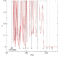
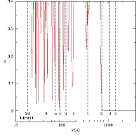
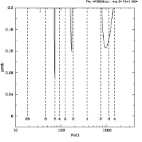
Figure 21: Same as Fig. 20 for the $P=2018$ d spectroscopic binary HIP 13055 (left panel) and for HIP 944 (middle panel) for which $P>800$ d may be inferred. For comparison, the right panel displays the $\alpha$ statistics for HIP 58596, a star with no evidence for binarity, neither from astrometry nor from spectroscopy (Jorissen et al., 2005; Drake and Pereira, 2008).

Thus, an interesting astrophysical outcome of the algorithm is a list of classical and metal-deficient barium stars shown to be astrometric binaries by the analysis of the Hipparcos IAD (Jorissen et al., 2005, 2004), and which were not subject to radial-velocity monitoring so far.

6.3 $\Delta\mu$ binaries: Comparing Hipparcos and Tycho-2 proper motions

Wielen (1997); Wielen et al. (1999) and Kaplan and Makarov (2003) suggested that the comparison of Hipparcos and Tycho-2 (Høg et al., 2000a, b) proper motions offers a way to detect binaries with long periods (typically from 1500 to 30000 d). The Hipparcos proper motion, being based on observations spanning only 3 yrs, may be altered by the orbital motion, especially for systems with periods in the above range whose orbital motion was not recognized by Hipparcos. On the other hand, this effect should average out in the Tycho-2 proper motion, which is derived from observations covering a much longer time span (Fig. 22). This method has been used by Wielen et al. (1999), Makarov (2004), Pourbaix (2004) and Frankowski et al. (2007).

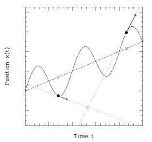
Figure 22: The orbital motion (solid line) of a binary, when sampled with a time span short with respect to the orbital period, may remain unnoticed, being an almost linear motion (represented by the arrows), adding to the proper motion of the centre of mass. On the contrary, when based on positional measurements covering a time span much longer than the orbital period, the proper motion will not be affected by the orbital motion, which averages out. (From (Wielen, 1997))

The method evaluates the quantity

$$\chi^{2}_{\rm obs}=(\vec{\mu}_{\rm HIP}-\vec{\mu}_{\rm Tyc})^{t}\;{\bf W}^{-1}\;(\vec{\mu}_{\rm HIP}-\vec{\mu}_{\rm Tyc}),$$ (27)

where $\vec{\mu}_{\rm HIP}$ and $\vec{\mu}_{\rm Tyc}$ are the vectors of $\alpha$ and $\delta$ components of the Hipparcos and Tycho-2 proper motions, respectively, and W is the associated $2\times 2$ variance-covariance matrix.

Since the above quantity follows a $\chi^{2}$ probability distribution function with 2 degrees of freedom, it is then possible to compute the probability Prob$(\chi^{2}>\chi^{2}_{\rm obs})$, giving the first kind risk of rejecting the null hypothesis $\vec{\mu}_{\rm Tycho}=\vec{\mu}_{\rm HIP}$ while it is actually true.

To evaluate the efficiency of the method, it has been applied by Frankowski et al. (2007) to all spectroscopic binary stars from the $S\!_{B^{9}}$ catalogue (Pourbaix et al., 2004a) with both an Hipparcos and a Tycho-2 entry. Figs. 23 and 24 show that the detection efficiency is very good in the period range 1500 - 30000 d for systems with parallaxes in excess of 10 – 20 mas. On the other hand, when the proper-motion method detects systems with orbital periods shorter than about 400 d, there is a good chance that the system is triple, the proper-motion method being sensitive to the long-period pair. This suspicion has been confirmed by Frankowski et al. (2007), and by Fekel et al. (2005, 2006) for the two ’textbook’ cases HIP 72939 and HIP 88848. Makarov and Kaplan (2005) and Frankowski et al. (2007) flagged these two stars as proper-motion binaries, despite the fact that the orbital periods known at the time are quite short, 3.55 and 1.81 d respectively. The discovery by Fekel et al. (2005, 2006) that these two systems are in fact triple, with long periods of 1641 and 2092 d, respectively, came as a nice a posteriori validation of the proper-motion method for identifying long-period binaries. The reprocessing of the Hipparcos data, accounting for the long-period pair, then yielded values for the Hipparcos proper motions perfectly consistent with the Tycho-2 ones, as it should. The situation is summarized in Table 2.

HIP 72939
$P=3.55$ and 1641 d
Fekel et al. (2006)
	Hipparcos	Tycho-2	Hip. reproc.
$\mu_{\alpha}\cos\delta$ (mas/yr)	$-67.5\pm 0.9$	$-66.2\pm 0.8$	$-67.0\pm 1.9$
$\mu_{\delta}$ (mas/yr)	$55.9\pm 0.9$	$62.1\pm 0.9$	$63.5\pm 1.5$
HIP 88848
$P=1.81$ and 2092 d
Fekel et al. (2005)
	Hipparcos	Tycho-2	Hip. reproc.
$\mu_{\alpha}\cos\delta$ (mas/yr)	$138.1\pm 1.9$	$108.5\pm 1.3$	$107.$
$\mu_{\delta}$ (mas/yr)	$-18.6\pm 1.7$	$-25.4\pm 1.2$	$-31$

Table 2: Two systems whose triple nature was first suspected by the proper-motion method and later confirmed by radial-velocity studies.

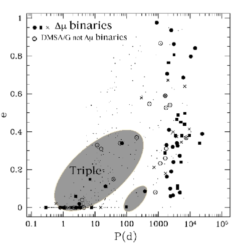
Figure 23: Eccentricity-period diagram for stars from the $S\!_{B^{9}}$ catalogue with parallaxes larger than 10 mas. Symbols are as follows: large filled symbols: proper-motion binaries detected at the 0.9999 confidence level, defined as $1-$Prob$(\chi^{2}>\chi^{2}_{\rm obs})$ (circles and squares denote those stars which are or are not, respectively, flagged as DMSA/G in the Hipparcos Catalogue, i.e., as stars with a non-linear proper motion); crosses: systems not flagged as DMSA/G, lying in the confidence-level range 0.99 – 0.9999; open circles: DMSA/G systems not flagged as proper-motion binaries at the 0.9999 level. (From (Frankowski et al., 2007))

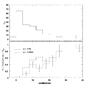
Figure 24: Upper left panel: Parallax distribution of $S\!_{B^{9}}$ stars with orbital periods larger than 1500 d. Lower left panel: Fraction of those $S\!_{B^{9}}$ stars detected as proper-motion binaries at confidence levels $\alpha$ of 0.99 and 0.9999. For parallaxes between 10 and 25 mas, about 50% of the $S\!_{B^{9}}$ stars with periods larger than 1500 d are detected, and that fraction becomes larger than 80% above 25 mas. Upper right panel: Orbital-period distribution for stars from the $S\!_{B^{9}}$ catalogue. Lower right panel: Fraction of stars in a given bin for which the Hipparcos and Tycho-2 proper motions differ at confidence levels of 0.9999 (dotted line) and 0.99 (dashed line). (From (Frankowski et al., 2007))

A very interesting side product of the proper-motion binary detection method is that, being totally independent of the star spectrum, it provides an unbiased estimate of the binary frequency among the different spectral classes. Table 3 reveals that the frequency of proper-motion binaries is constant within the error bars (at least in the range F to M). According to Frankowski et al. (2007), proper-motion binaries represent about 35% of the total number of spectroscopic binaries, because of their more restricted period range. Thus, the frequencies of proper-motion binaries listed in Table 3 can be multiplied by 1/0.35 = 2.86 to yield the total fraction of spectroscopic binaries, namely 28.8%. This value is close to the spectroscopic-binary frequency of $30.8\pm 1.7$% for cluster K giants found by Mermilliod et al. (2007).

Table 3: The frequency of proper-motion binaries among different spectral classes, from Frankowski et al. (2007). $N$ is the total number of stars of the corresponding spectral type in the sample.

Spectral type	%	$N$
B	$14.3\pm 13.2$	8664
A	$15.2\pm 3.0$	15662
F	$11.4\pm 1.0$	21340
G	$10.5\pm 0.8$	19628
K	$9.3\pm 0.7$	29349
M	$9.8\pm 1.3$	4217
All	$10.1\pm 0.4$	103304

6.4 Variability-Induced Movers and Color-induced displacement binaries

The two methods presented in this section are unusual in the sense that they combine photometry and astrometry to diagnose a star as a binary.

The first category, Variability-Induced Movers, is defined in the Double and Multiple System Annex (DMSA) of the Hipparcos Catalogue, where it is known as DMSA/V. Stars flagged as DMSA/V are generally large-amplitude variables whose residuals with respect to a single-star astrometric solution are correlated with the star apparent brightness. Such a situation may arise in a binary system, when the position of the photocentre of the system varies as a result of the light variability of one of its components: when the variable component is at maximum light, it dominates the system light, and the photocentre position is closer to the position of that star (Wielen, 1996, see also Eq. 20). Pourbaix et al. (2003) have shown, however, that many of the long-period variables DMSA/V listed in the Hipparcos Catalogue are not binaries, the correlation of the astrometric residuals with the stellar brightness resulting in fact from the colour variation accompanying the light variation of a long-period variable. This colour variation was not accounted for in the standard processing applied by the Hipparcos reduction consortia, which adopted a constant colour for every star. Thus, the so-called chromaticity effect (for a given position on the sky, the position of a star on the Hipparcos focal plane depends on the star colour, because of various chromatic aberrations in the Hipparcos optical system) was not appropriately corrected in the case of long-period variables. When this effect is incorporated in the astrometric processing (by using epoch colours; Platais et al., 2003), a single-star solution appears to appropriately fit the observations for 161 among the 188 stars originally flagged as DMAS/V in the Hipparcos Catalogue, as shown by Pourbaix et al. (2003). The 27 remaining DMSA/V may be true binaries, and are listed in Table 4.

Table 4: The 27 stars keeping their DMSA/V status after the appropriate re-processing by Pourbaix et al. (2003). They may be true binaries. The column labelled ’Var’ lists the variability type (M = Mira; SR = semi-regular; L = irregular).

HIP	GCVS	Var	Rem
781	SS Cas	M
2215	AG Cet	SR
11093	S Per	SRc
23520	EL Aur	Lb
31108	HX Gem	Lb:
36288	Y Lyn	L
36669	Z Pup	M
41058	T Lyn	M
43575	BO Cnc	Lb:
45915	CG UMa	Lb
46806	R Car	M	$V=11.3$ companion located 1.8” away
54951	FN Leo	L
67410	R CVn	M
68815	$\theta$ Aps	SRb
75727	GO Lup	SRb
76377	R Nor	M
79233	RU Her	M	composite spectrum ?
80259	RY CrB	SRb
90709	SS Sgr	SRb
93605	SU Sgr	SR
94706	T Sgr	M	composite spectrum
95676	SW Tel	M
99653	RS Cyg	SRa
100404	BC Cyg	L
109089	RZ Peg	M
111043	$\delta^{2}$ Gru	Lb:
112961	$\lambda$ Aqr	L

Colour-induced displacement binaries are detected when the position of the photocentre depends on the considered photometric band, after correcting for any instrumental chromatic effect (Christy et al., 1983). This situation is analogous to the previous one, except that the light variability of one component is here replaced by the colour difference between the two stars: if the two components of a binary system have very different colours, the respective contribution of each component to the integrated system light will be different in the different photometric bands, and so will be the position of the photocentre. This method thus requires accurate astrometry in various filters and is able to detect only binary systems with components of very different spectral types. The former condition is met by the Sloan Digital Sky Survey (SDSS; Adelman-McCarthy et al., 2007), which provides positions in the Gunn system $u,g,r,i,z$ (Fig. 25). The latter condition is met by white-dwarf/red-dwarf pairs. Pourbaix et al. (2004b) found 346 pairs among the $4.1\;10^{6}$ stars with $u,g<21$ in the second SDSS data release (Adelman-McCarthy et al., 2007) with a distance between the $u$ and $z$ positions larger than $0.5^{\prime\prime}$. Most (about 90%) of these must indeed correspond to red-dwarf/white-dwarf pairs, as indicated on Fig. 26, the remaining 10% being probably early main-sequence/red-giant pairs.

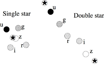
Figure 25: Schematic position of the photocentre in the different SDSS bands. Right panel: For double stars, the positions are aligned along the line joining the two stars and are ordered according to the central wavelength of the filter. The true positions of the stars are represented as a five-branch star symbol. Left panel: For single stars, measurement errors prevent the positions from being perfectly superimposed. (From (Pourbaix et al., 2004b))

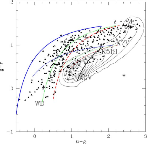
Figure 26: Color-color diagram of the putative binaries (triangles) superimposed on the original parent population from the second SDSS data release (contours). The thick lines on the left correspond to systems with an M dwarf and three different kinds of WDs. Thin lines are the same, but for a K7V star instead of an M dwarf. The short thick solid line in the centre, overlapping the density contours, corresponds to A0V/K5III pairs. (From (Pourbaix et al., 2004b))

7 Other detection methods

7.1 Detecting binaries from rapid rotation

Another method for finding binaries (among old, late-type stars) involves the identification of fast rotators, since evolved late-type stars are not expected to rotate fast (see e.g. De Medeiros et al., 1996; De Medeiros and Mayor, 1999). Fast rotation can be ascribed to spin-up processes operating either in tidally interacting systems (like RS CVn systems among K giants; De Medeiros et al., 2002), or in mass-transfer systems, through transfer of spin angular momentum.

In recent years, the link between rapid rotation of old, late-type stars and spin-accretion during (wind) mass transfer in binaries has been strengthened, most notably by the discovery of the family of WIRRing stars (standing for ’Wind-Induced Rapidly Rotating’; Jeffries and Stevens, 1996). Originally, this class was defined from a small group of rapidly-rotating, magnetically-active K dwarfs with hot WD companions discovered by the ROSAT Wide Field Camera and Extreme Ultraviolet Explorer (EUVE) surveys (Jeffries and Stevens, 1996; Jeffries and Smalley, 1996; Vennes et al., 1997). Since these stars exhibit no short-term radial-velocity variations, it may be concluded that any orbital period must be a few months long at least. Moreover, several arguments, based on proper motion, WD cooling time scale, and lack of photospheric Li, indicate that the rapid rotation of the K dwarf cannot be ascribed to youth. Jeffries and Stevens (1996) therefore suggested that the K dwarfs in these wide systems were spun up by the accretion of the wind from their companion, when the latter was a mass-losing AGB star. The possibility of accreting a substantial amount of spin from the companion’s wind has been predicted Theuns and Jorissen (1993); Theuns et al. (1996); Mastrodemos and Morris (1998) by smooth-particle hydrodynamics simulations of wind accretion in detached binary systems. A clear signature that mass transfer has been operative in the WIRRing system 2RE J0357+283 is provided by the detection of an overabundance of barium Jeffries and Smalley (1996). Interestingly enough, the class of WIRRing stars is no more restricted to binaries with a late dwarf primary, since in recent years, WIRRing systems were found among many different classes of stars:

• A number of barium stars (post-mass-transfer systems involving a K giant and a WD) have been found to rotate fast, with in some cases (HD 165141 and 56 Peg; Jorissen et al., 1996; Frankowski and Jorissen, 2006) clear indications that the mass transfer responsible for the chemical pollution of the atmosphere of the giant has occurred recently enough for the magnetic braking not to have slowed down the giant appreciably. These systems thus exhibit signatures of X-ray activity comparable to RS CVn systems (HD 165141, 56 Peg) or host a warm, relatively young WD (HD 165141). HD 77247 is another barium star with broad spectral lines (Jorissen et al., 1998). It could thus be a fast rotator, but it has no other peculiarity, except for its outlying location in the eccentricity – period diagram ($P=80.5$ d; $e=0.09$). In this case, the fast rotation could thus rather be the result of tidal synchronization.

• Among binary M (or C) giants, V Hya, HD 190658 and HD 219654 are fast rotators (respectively with $V\sin i=16$ km s^-1, $15.1\pm 0.1$ km s^-1 and $13.6\pm 0.8$ km s^-1) (Famaey et al., 2008; Knapp et al., 1999). HD 190658 is the M-giant binary with the second shortest period known so far (199 d; (Famaey et al., 2008)), and exhibits as well ellipsoidal variations (Samus, 1997). Fast rotation is therefore expected in such a close binary with strong tidal interactions. The radius derived under the assumption of a rotation synchronized with the orbital motion is then $R\sin i=59$ R_⊙, corresponding to $R/a_{1}=1.16$, where $a_{1}$ is the semi-major axis of the giant’s orbit around the centre of mass of the system (Lucke and Mayor, 1982). The radius deduced from Stefan-Boltzmann law is 62.2 R_⊙ (Frankowski et al., 2008), which implies an orbit seen very close to edge-on ($\sin i=0.948$ or $i=71.4^{\circ}$). Adopting typical masses of 1.7 M_⊙ for the giant and 1.0 M_⊙ for the companion, one obtains $R/a=0.43$ and $R/R_{R}=1$ ! Thus, the star apparently fills its Roche lobe.

• Binary nuclei of planetary nebulae of the Abell-35 kind (containing only four members so far: Abell 35 = BD$-22^{\circ}$3467 = LW Hya, LoTr 1, LoTr 5 = HD 112313 = IN Com = 2RE J1255+255, and WeBo 1 = PN G135.6+01.0) have their optical spectra dominated by late-type (G-K) stars (with demonstrated barium anomaly in the case of WeBo 1 only; Gatti et al., 1997; Thevenin and Jasniewicz, 1997; Bond et al., 2003; Pereira et al., 2003), but the UV spectra reveal the presence of extremely hot ($>$ 10⁵ K), hence young, WD companions. A related system is HD 128220, consisting of an sdO and a G star in a binary system of period 872 d Howarth and Heber (1990). In all these cases, the late-type star is chromospherically active and rapidly rotating, and this rapid rotation is likely to result from a recent episode of mass transfer.

• Rapid rotation seems to be a common property of the giant component in the few known symbiotics of type d’ (Jorissen et al., 2005; Zamanov et al., 2006). The evolutionary status of this rare set of yellow d’ symbiotic systems (SyS), which were all shown to be of solar metallicity, has recently been clarified (Jorissen et al., 2005) with the realisation that in these systems, the companion is intrinsically hot (because it recently evolved off the AGB), rather than being heated by accretion or nuclear burning as in the other brands of SyS. Several arguments support this claim: (i) d’ SyS host G-type giants whose mass loss is not strong enough to heat the companion through accretion and/or nuclear burning; (ii) the cool dust observed in d’ SyS (Schmid and Nussbaumer, 1993) is a relic from the mass lost by the AGB star; (iii) the optical nebulae observed in d’ SyS are most likely genuine PN rather than the nebulae associated with the ionized wind of the cool component (Corradi et al., 1999). d’ SyS often appear in PN catalogues. AS 201 for instance actually hosts two nebulae (Schwarz, 1991): a large fossil planetary nebula detected by direct imaging, and a small nebula formed in the wind of the current cool component; (iv) rapid rotation has likely been caused by spin accretion from the former AGB wind like in WIRRing systems. The fact that the cool star has not yet been slowed down by magnetic braking is another indication that the mass transfer occurred fairly recently. Corradi and Schwarz (1997) obtained 4000 y for the age of the nebula around AS 201, and 40000 y for that around V417 Cen.

• The blue stragglers were first identified by Sandage (1953) in the globular cluster M3. Since their discovery, blue stragglers have been found in many other globular clusters and in open clusters as well. The frequency of blue stragglers is also correlated with position in clusters (see Carney et al., 2005, and references therein). Depending on the cluster, this frequency may either increase or decrease with the distance from the centre, thus calling for two different mechanisms for the creation of blue stragglers in clusters. In the central regions, dynamical effects involving collisions may enhance the probabilities for creating blue stragglers (Sills and Bailyn, 1999). In the outer regions, where binary systems are most likely to survive, mass transfer is a likely explanation (McCrea, 1964; Mateo et al., 1990). Despite being initially found in the globular clusters, blue stragglers are now found as well in the (halo) field where they are known as either ’blue metal-poor stars’ (Preston et al., 1994; Preston and Sneden, 2000; Sneden et al., 2003) or ’ultra-Li-deficient stars’ (Ryan et al., 2001, 2002). The very large binary frequency among these classes of stars (Carney et al., 2005; Preston and Sneden, 2000; Sneden et al., 2003; Carney et al., 2001) strongly suggests that field blue stragglers result from mass transfer in a binary, rather than from the various merger processes that are currently believed to produce blue stragglers in the inner regions of globular clusters.

  Finally coming to the issue at stake in this section, Carney et al. (2005), Preston and Sneden (2000) and Ryan et al. (2002) find that the field blue straggler stars that are binaries have higher rotational velocities than stars of comparable temperature but showing no evidence of binarity. Moreover, the orbital periods are too long for tidal effects to be important, implying that spin-up during mass transfer when the orbital separations and periods were smaller is the cause of the enhanced rotation. This conclusion is supported by the abnormally high proportion of blue-metal-poor binaries with long periods and small orbital eccentricities, properties that these binaries share with barium stars and related binaries (Preston and Sneden, 2000). Fuhrmann and Bernkopf (1999) likewise draw a connection between rapid rotation, Li depletion, and mass transfer from a companion in rather long-period systems (several hundred days).

7.2 X-rays

Several physical processes, which will be discusssed below, are responsible for the emission of X-rays in binaries, so that their detection provides a useful diagnostic of binarity. In single stars, X-rays are only expected in stars located to the left of the Linsky-Haisch line in the Hertzsprung-Russell diagram (Linsky and Haisch, 1979; Haisch et al., 1991), separating warm stars with hot coronae from cool stars with wind mass loss (Fig. 27). Exceptions to this rule are, however, M dwarfs rotating rapidly because they are young, thus producing a dynamo effect which may heat the corona.

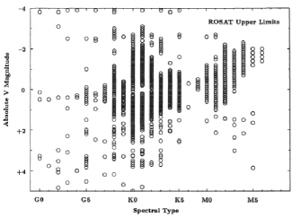
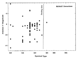
Figure 27: Comparison of the location in the Hertzsprung-Russell diagram of stars with and without X-rays detected by the ROSAT satellite (right and left panels, respectively). The ’dividing line’ is clearly apparent on the right panel. (From (Haisch et al., 1991))

X-rays (corresponding to photons with $h\nu>0.1$ keV requiring $T>10^{6}$ K) may come from:

• hot stellar coronae heated by a dynamo triggered by fast rotation (Pallavicini et al., 1981), either due to youth, or to synchronous rotation in a close binary system (as in RS CVn systems; Eaton and Hall, 1979).

• nuclear fusion at the surface of a WD (as in novae or symbiotic stars). In classical novae, explosive H-burning (releasing $10^{33}-10^{34}$ erg s^-1) occurs, whereas in ’super soft sources’ (as are symbiotic stars), it is probably quiescent H-burning.

• accretion in binary systems like

  • cataclysmic variables (CVs, consisting of a dwarf star and a WD in a semi-detached system with periods of a few hours), which themselves subdivide into

    • Classical novae, some can be detected in X-rays outside of eruptions;

    • Dwarf novae, with outburst powered by accretion-disk instability;

    • Polars (AM Her systems), involving highly magnetized WDs around which no accretion disk can form because of the very strong magnetic field;

    • Intermediate Polars (DQ Her systems), involving highly magnetized WDs in a rather wide system which allows some room for an accretion disk restricted to the outer region of the Roche lobe; in the inner region, no accretion disk can form because of the very strong magnetic field;

  • Algols (which are semi-detached systems consisting of a subgiant component and a more massive main sequence component);

  • symbiotic systems, consisting of a giant star and a WD in a system with a period exceeding 100 d. However, as we discuss below, the accretion-driven nature of the X-rays emitted by SyS has been debated.

• wind collision, as in SyS.

7.2.1 X-rays from binaries: The case of SyS

One of the defining properties of SyS is to host a hot compact star, generally a WD, accreting matter from a giant companion (Corradi et al., 2003). The WD is heated either directly by accretion, or indirectly by nuclear burning fueled by accretion (Jorissen, 2003b, and references therein). Symbiotic stars are X-ray sources (Mürset et al., 1997), at the level $10^{30}$ to $10^{33}$ erg s^-1. The physical process emitting these X-rays in symbiotic stars is still debated, though. Direct evidence for the presence of an accretion disk, in the form of continuum flickering and far UV continuum is not usually found in symbiotic stars (Sokoloski et al., 2001; Sokoloski, 2003; Sion, 2003), unlike the situation prevailing in cataclysmic variables and low-mass X-ray binaries (Sokoloski et al., 2001; Guerrero et al., 2001). Z And is the only SyS where the accretion-driven nature of X-rays makes no doubt, because flickering on time scales ranging from minutes to days has been observed (Sokoloski, 2003). Other mechanisms were therefore advocated to account for the X-ray emission from SyS, like thermal radiation from the hot component in the case of supersoft X-ray sources, or the shock forming in the collision region between the winds from the hot and cool components (Mürset et al., 1997). Interestingly, Soker (2002) even suggests that the X-ray flux from SyS exclusively arises from the fast rotation of the cool component spun up by wind accretion from the former AGB component (now a WD)! If that hypothesis is correct, the properties of X-rays from SyS would be undistinguishable from those of active (RS CVn-like) binaries. It is an intriguing hypothesis, because it requires a high incidence of fast rotation among SyS, which has so far only been reported for d’ symbiotics (see above and Zamanov et al., 2006).

The barium system 56 Peg provides an interesting illustration of the difficulty of finding the exact origin of the emitted X-rays. X-rays were detected with the Einstein satellite by Schindler et al. (1982). In a subsequent study, Dominy and Lambert (1983) attributed the X-rays to an accretion disk around the WD companion. Frankowski and Jorissen (2006) re-interpreted the X-rays as due to RS CVn-like activity, because the recent finding by Griffin (2006) that the orbital period of the system is as short as 111 d can only be reconciled with other properties of 56  Peg if it is a fast rotator seen almost pole-on! Its X-ray luminosity is consistent with the rotation-activity relationship of Pallavicini et al. (1981), provided that it rotates at a velocity of about 50 km s^-1 (Fig. 28) (despite an observed value $V_{\rm rot}\sin i$ of only 4.4 km s^-1; De Medeiros and Mayor, 1999), thus implying an almost pole-on orbit. A low inclination is also required by evolutionary considerations, in order to allow the companion of this barium star to be a WD, given the very low mass function obtained by Griffin (2006): $f(M)=3.73\;10^{-5}$ M_⊙.

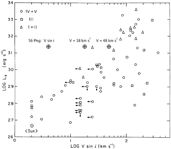
Figure 28: X-ray luminosities vs. projected rotational velocities for 56 Peg (encircled crosses, for $V\sin i$ and for two values of $V$: assuming orbital corotation or fast rotation) and stars of various spectral types and luminosity classes detected by the Einstein Observatory. Different symbols indicate different luminosity classes, as indicated in the figure. (Adapted from (Frankowski and Jorissen, 2006) and (Pallavicini et al., 1981)).

Given the small orbital separation, one may still wonder whether there should not be as well some contribution to the X-ray flux coming from accretion, as advocated by Schindler et al. (1982) and Dominy and Lambert (1983). The major evidence suggesting that there may be a link between mass transfer and X-ray emission in active binaries is the correlation between the X-ray luminosity and the Roche-lobe filling fraction $\gamma_{2}$ for RS CVn systems noted by Welty and Ramsey (1995). Singh et al. (1996) re-examined this issue using samples of RS CVn and Algol binaries, and confirm the weak correlation found earlier by Welty and Ramsey (1995). However, Singh et al. “regard this as a rather weak argument, because both the X-ray luminosities and the Roche lobe filling fractions are themselves correlated with the stellar radii in the sample of RS CVn binaries, and thus regard this correlation as merely a by-product of the inherent size dependence of these quantities.” Actually, despite the short orbital period, the filling factor of 56 Peg A is not that close to unity.

7.3 Composite spectra and magnitudes

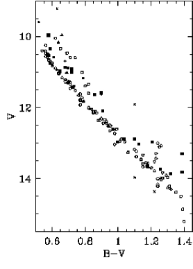
Figure 29: Left panel: Theoretical zero-age single star and equal-mass binary main sequences for a metallicity of $Z=0.02$ covering a range of absolute magnitudes $M_{V}$. Also plotted for a range of primary masses, $M_{1}$, are binary points with $M_{2}=qM_{1}$ where $q$ ranges from $1.0\rightarrow 0.0$ in increments of 0.1. The point at $q=0.5$ is an open square. (From (Hurley and Tout, 1998)). Right panel: The $(V,B-V)$ color-magnitude diagram for low-mass Praesepe members. Symbols are as follows: filled squares: optically-resolved binary systems; filled dots: known spectroscopic binaries; filled triangles: triple systems; open circles: ’single’ stars (although some of these are resolved in the infrared); crosses : suspected non members. (From (Bouvier et al., 2001))

SyS are a specific example of a more general class of binaries having composite spectra, where the spectral features of the two components are intermingled. Spectroscopically, these systems correspond to SB2 binaries. Ginestet et al. (1997) and Ginestet and Carquillat (2002) provide lists of more than 100 systems with true composite spectra of various spectral types and luminosity classes.

In color-color and color-magnitude diagrams, these stars occupy outlying positions and may therefore be easily identified. In colour-magnitude diagrams of clusters for instance, binaries widen the main sequence. This effect has been quantified by Hurley and Tout (1998), as shown on the left panel of Fig. 29. A beautiful illustration of this effect is provided by the color-magnitude diagram of the Praesepe open cluster where the binary sequence is clearly apparent (Right panel of Fig. 29).

7.4 Detecting binaries from the partial absence of maser emission

Maser emission is observed in many LPVs, and corresponds to stimulated molecular emission from an upper level which is more populated than the lower level (population inversion). For a review of physical processes related to astronomical masers, we refer to the textbook by Elitzur (1992). The maser emission originates from gas in the circumstellar nebula (fed, e.g., by the strong stellar wind of late-type giants) and involves various molecules: SiO, H₂O and OH in O-rich environments, and mostly HCN in C-rich environments. Depending on the energy required to populate the upper level, the maser emission will originate from regions closer or farther away from the central star. As discussed by Elitzur (1992) and Lewis (1989), the SiO maser requires the highest excitation energies (with the involved levels lying at energies between $k\times 1730$ K and $k\times 5500$ K, where $k$ is the Boltzmann constant) and thus originates at the closest distances from the star. The H₂O maser requires intermediate excitation temperatures (the involved levels correspond to $E/k$ between 300 and 1900 K), and operates at intermediate distances from the star, whereas the OH maser (subdivided into the so-called main OH maser at frequencies 1665 and 1667 MHz, and the satellite line 1612 MHz OH maser) involves levels with low excitation temperatures ($\sim 200$ K). Therefore, when the three O-bearing masers operate concurrently in a circumstellar shell, they do so at different distances from the central star. A textbook example is provided by the supergiant star VX Sgr (Fig. 30; Chapman and Cohen, 1986).

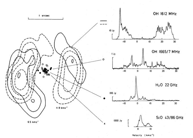
Figure 30: The maser emission around the supergiant star VX Sgr. The solid and dashed lines correspond to contours of iso-intensity for the 1612 MHz OH maser line, for gas line-of-sight velocities of 6.5 and 11.9 km s^-1, respectively. The stellar velocity is 5.5 km s^-1. (From (Chapman and Cohen, 1986))

The role of binarity in suppressing the maser activity was suspected on theoretical grounds (Herman and Habing, 1985), since the presence of a companion periodically disturbs the layer where maser activity should develop. The systematic absence of SiO masers in symbiotic stars except in the very wide system R Aqr (Schwarz et al., 1995; Hinkle et al., 1989) is evidence supporting that claim. On the other hand, very wide systems like o Ceti, R Aqr and X Oph (Jorissen, 2003a) lack the OH maser, which involves layers several $10^{5}$ R_⊙ away from the star, in contrast to the SiO maser, which forms close to the photosphere. There should actually be a critical orbital separation for every kind of maser below which the companion sweeps through the corresponding masing layer (Schwarz et al., 1995), thus preventing its development ($A$ $<$ 10 AU: no masing activity; 10 $\leq$ $A{\rm(AU)}$ $<$ 50: SiO and H₂O masers possible but no OH maser; $A$ $>$ 50 AU: all masers can operate).

A survey of IRAS sources by Lewis et al. (1987) reveals that the region occupied by OH/IR sources in the IRAS color–color diagram also contains many stars with no OH masing activity. Furthermore, detected and undetected OH maser sources have identical galactic latitude distributions. These two facts find a natural explanation if binarity is the distinctive property between detections and nondetections.

Lewis (1989) (see also Stencel et al., 1990) has presented a chronological sequence of maser states, with increasing mass loss and thus shell thickness. The SiO maser, H₂O maser, the main OH maser and finally the 1612 MHz OH maser are added one by one as the shell grows in thickness. This sequence is supported by the fact that SiO and H₂O masers are associated with optically identified stars, while the majority of 1612 MHz OH maser sources lack an optical counterpart (OH/IR sources). The masers then disappear in the reverse order as the shell continues to thicken, with the exception of the 1612 MHz OH maser, which remains strong. The SiO maser disappears once steady mass loss stops. Thereafter, the main OH maser eventually reappears and grows rapidly in strength relative to the 1612 MHz maser in the detached fossil shell, until its ongoing dilation causes all of the OH masers to fade away.

Anomalies in this chronological sequence may be another indication that the star has a companion which sweeps through the layer where the lacking maser should operate. Therefore, a search for binaries among late-type giants involves looking in maser catalogues (Benson et al., 1990) for O-rich stars with SiO and OH masers but no H₂O maser, since this combination is never encountered in Lewis (1989) chronological sequence. RU Her is an example of such an anomaly; it is therefore quite significant that this star is suspected to have a composite spectrum (Herbig, 1965) and appears in Table 4 as a true ’Variability-Induced Mover’, which are two further indications of its binary nature.

Table 5: A summary of the different properties that may be derived for the various classes of binaries. The symbols $R_{A}$ and $d$ denote the radius of the eclipsed component A and the distance of the system from the Sun, respectively.

Binaries	Visual	Astrometric		Spectroscopic		Eclipsing
		AB1	AB2	SB1	SB2
Max $P$ $\sim$	..	100 yr		30 yr		$\sim$ 1 yr
Min $P$ $\sim$	1 yr	1 yr		1 d		1 h
$i$ ?	yes	yes	yes	no	no	yes
$a$ ?	$a_{A}+a_{B}$	$a_{0}$	$a_{A,B}$	$a_{A}\sin i$	$a_{A,B}\sin i$	$a$
(units)	(”)	(”)	(”)	(km)	(km)	($R_{A}$)
Masses	$(M_{A}+M_{B})d^{-3}$	—	$M_{A,B}$	$f(M)$	$M_{A,B}\sin^{3}i$	$(M_{A}+M_{B})R_{A}^{-3}$
AB2 systems (Sirius, $\alpha$ Cen) are rare (Demarque et al., 1986)
Ecl + SB2 (Ex: HD 35155): individual masses may be derived

8 What may be known about stellar masses?

Binary stars are often considered as the golden way to derive stellar masses. Table 5 shows, however, that the different binary-detection methods actually offer only partial knowledge of the masses. It is only when a given system appears as both eclipsing and SB2 that the individual masses may be derived. We refer to Andersen (1991) for a detailed review on this topic.

9 A list of resources on binary stars

9.1 Combined data

The best entry point of any search about binary stars is probably the Besançon database http://bdb.obs-besancon.fr/, which provides links to most of the catalogues and databases listed in this section.

A yearly bibliography about double stars is available at
http://ad.usno.navy.mil/wds/dsl/bib’nnnn’.html
(where ’nnnn’ = 2006 for instance).

9.2 IAU commissions of interest

• IAU commission 8 : Astrometry
  http://www.ast.cam.ac.uk/iau_comm8/

• IAU commission 26 : Binary and Multiple Stars
  http://ad.usno.navy.mil/wds/dsl.html#iau

• IAU commission 27 : Variable Stars
  http://www.konkoly.hu/IAUC27/

• IAU commission 30 : Radial velocities
  http://www.ctio.noao.edu/science/iauc30/iauc30.html

• IAU commission 42 : Close Binary Stars
  http://www.konkoly.hu/IAUC42/c42info.html

9.3 Visual and interferometric binaries

• Library of links: CHARA (integrates many sources: interferometric, speckle or occultation data, WDS, Hipparcos DMSA)
  http://ad.usno.navy.mil/wds/dsl.html
  

• Instantaneous positions:

  • Catalogue of Interferometric Measurements of Binary Stars
    http://ad.usno.navy.mil/wds/int4.html

  • CCDM
    http://webviz.u-strasbg.fr/viz-bin/Vizier?-source=I/274

  • Washington Double Stars (WDS)
    http://ad.usno.navy.mil/wds/wds.html

  • SIDONIE
    http://sidonie.obs-nice.fr

• Orbits:
  Sixth Catalogue of Orbits of Visual Binary Stars (Hartkopf & Mason)
  http://ad.usno.navy.mil/wds/orb6.html

9.4 Spectroscopic binaries

• Spectral families

  • Barium stars (Lü et al., 1983):
    http://cdsads.u-strasbg.fr/full/1983ApJS...52..169L

  • S stars (Stephenson, 1984):
    http://vizier.u-strasbg.fr/viz-bin/VizieR?-source=III/168

  • C stars (Alksnis et al., 2001):
    http://vizier.u-strasbg.fr/viz-bin/VizieR?-source=III/227

  • Metal-deficient barium and CH stars (Šleivyte and Bartkevičius, 1990; Bartkevic̃ius, 1996):
    http://cdsads.u-strasbg.fr/abs/1990VilOB..85....3S

  • Cataclysmic binaries and X-ray binaries (Ritter and Kolb, 2003):
    http://physics.open.ac.uk/RKcat/ (update RKcat7.8, 2007)

  • Chromospherically active binaries (Strassmeier et al., 1993):
    http://vizier.u-strasbg.fr/viz-bin/VizieR?-source=V/76

  • Symbiotic stars

    • http://vizier.u-strasbg.fr/viz-bin/VizieR?-source=J/A+AS/146/407 (Belczyński et al., 2000)

    • See as well the series of papers by Carquillat (Carquillat and Prieur, 2008), R.E. Griffin (Griffin et al., 2006b), Ginestet (Ginestet et al., 1997; Ginestet and Carquillat, 2002)

• Individual radial-velocity measurements
  http://www.casleo.gov.ar/catalogo/catalogo.htm
  

• Orbits:
  The 9th Catalogue of Spectroscopic Binary Orbits (Pourbaix et al., 2004a)
  http://sb9.astro.ulb.ac.be/

9.5 Astrometric binaries

• Common proper-motion pairs:

  • Luyten LDS catalogue
    http://vizier.u-strasbg.fr/viz-bin/VizieR?-source=I/130

  • Halbwachs 1986 (Halbwachs, 1986)
    http://vizier.u-strasbg.fr/viz-bin/VizieR?-source=I/121

  • Greaves 2004 (Greaves, 2004)
    http://vizier.u-strasbg.fr/viz-bin/VizieR?-source=J/MNRAS/355/585

• $\Delta\mu$ binaries:

  • DMUBIN database (Wielen et al., 1999)
    http://www.ari.uni-heidelberg.de/datenbanken/dmubin

  • Makarov & Kaplan 2005 (Makarov and Kaplan, 2005)

  • Frankowski et al. 2007 (Frankowski et al., 2007)

• Hipparcos: DMSA/O binaries

9.6 Photometric variables

• General Catalogue of Photometric Data
  http://obswww.unige.ch/gcpd/gcpd.html

• Hipparcos photometry annex
  http://www.rssd.esa.int/SA/HIPPARCOS/apps/PlotCurve.html

• All Sky Automated Survey
  http://archive.princeton.edu/ asas/

• Northern Sky Variability Survey
  http://skydot.lanl.gov/

• OGLE
  http://bulge.princeton.edu/$\sim$ogle/

• MACHO
  http://wwwmacho.mcmaster.ca/

• DENIS
  http://www-denis.iap.fr

• Eclipsing binaries:

  • http://cdsweb.u-strasbg.fr/cgi-bin/myqcat3?eclipsing+binaries

  • Krakow Observatory
    http://www.oa.uj.edu.

  • Contact (W UMa-type) binaries at Konkoly Observatory
    http://www.konkoly.hu/staff/csizmadia/wuma.html

  • A catalogue of eclipsing variables (Malkov et al., 2006)

• AAVSO
  http://www.aavso.org

• also look for the sites of the French, British, Swiss, New Zealander variable-star-observer associations…

References

- Eggleton (2006) P. Eggleton, Evolutionary Processes in Binary and Multiple Stars, Cambridge University Press, 2006.
- Shore (1994) S. N. Shore, “Observations and Physical Processes in Binary Stars” in Interacting Binaries (Saas-Fee Advanced Course 22), edited by S. N. Shore, M. Livio, and E. van den Heuvel, Springer-Verlag, Berlin, 1994, p. 1.
- Argyle (2004) B. Argyle, Observing and Measuring Visual Double Stars, Springer, London, 2004.
- Jorissen (2003a) A. Jorissen, “Binary AGB Stars and their Progeny” in Asymptotic Giant Branch Stars, edited by H. Habing, and H. Olofsson, Springer Verlag, New York, 2003a, pp. 461–518.
- Frankowski and Jorissen (2007) A. Frankowski, and A. Jorissen, Baltic Astronomy 16, 104–111 (2007).
- Lattanzio and Wood (2003) J. C. Lattanzio, and P. Wood, “Evolution, Nucleosynthesis, and Pulsation of AGB Stars” in Asymptotic Giant Branch Stars, edited by H. Habing, and H. Olofsson, Springer Verlag, New York, 2003, p. 23.
- McClure (1984) R. D. McClure, PASP 96, 117–127 (1984).
- Bond et al. (1993) H. E. Bond, R. Ciardullo, and M. G. Meakes, “The Abell 35-Type Planetary Nuclei” in Planetary Nebulae (IAU Symp. 155), edited by R. Weinberger, and A. Acker, Kluwer, Dordrecht, 1993, p. 397.
- Jeffries and Stevens (1996) R. D. Jeffries, and I. R. Stevens, MNRAS 279, 180–190 (1996).
- McClure (1984) R. D. McClure, ApJ 280, L31 (1984).
- McClure (1997) R. D. McClure, PASP 109, 536 (1997).
- Jorissen and Mayor (1992) A. Jorissen, and M. Mayor, A&A 260, 115 (1992).
- Schmid and Nussbaumer (1993) H. M. Schmid, and H. Nussbaumer, A&A 268, 159–177 (1993).
- Van Winckel (2003) H. Van Winckel, ARA&A 41, 391–427 (2003).
- Van Winckel (2007) H. Van Winckel, Baltic Astronomy 16, 112 (2007).
- Jorissen (2003b) A. Jorissen, “The Link between Symbiotic Stars and Chemically Peculiar Red Giants” in Symbiotic stars probing stellar evolution, edited by R. L. M. Corradi, J. Mikołajewska, and T. J. Mahoney, Astron. Soc. Pacific Conf. Ser. Vol. 303, San Francisco, 2003b, p. 25.
- Parthasarathy et al. (2007) M. Parthasarathy, D. Branch, D. J. Jeffery, and E. Baron, New Astronomy Review 51, 524–538 (2007).
- Jorissen et al. (2005) A. Jorissen, L. Začs, S. Udry, H. Lindgren, and F. A. Musaev, A&A 441, 1135–1148 (2005).
- Clayton (1988) D. D. Clayton, MNRAS 234, 1–36 (1988).
- Drake and Pereira (2008) N. A. Drake, and C. B. Pereira, AJ 135, 1070–1082 (2008).
- Masseron et al. (2006) T. Masseron, S. Van Eck, B. Famaey, S. Goriely, B. Plez, L. Siess, T. Beers, F. Primas, and A. Jorissen, A&A 455, 1059–1072 (2006).
- Van Eck et al. (2003) S. Van Eck, S. Goriely, A. Jorissen, and B. Plez, A&A 404, 291–299 (2003).
- Binnendijk (1960) L. Binnendijk, Properties of double stars - A survey of parallaxes and orbits, University of Pennsylvania Press, Philadelphia, 1960.
- Heintz (1979) W. Heintz, Double Stars, Reidel, Dordrecht, 1979.
- Eggleton (1983) P. P. Eggleton, ApJ 268, 368 (1983).
- Schuerman (1972) D. W. Schuerman, Ap&SS 19, 351 (1972).
- Dermine and Jorissen (2008) T. Dermine, and A. Jorissen, A&A, in preparation (2008).
- Vogel (1890) H. C. Vogel, Astron. Nach. 123, 289 (1890).
- Pickering (1890) E. C. Pickering, Am. J. Science 39, 46 (1890).
- Smart (1977) W. M. Smart, Textbook on Spherical Astronomy, Cambridge University Press, Cambridge, 1977.
- Andersen (1991) J. Andersen, A&A Rev. 3, 91–126 (1991).
- Udry et al. (1998) S. Udry, A. Jorissen, M. Mayor, and S. Van Eck, A&AS 131, 25–41 (1998).
- Ake et al. (1991) T. B. Ake, H. R. Johnson, and M. M. Ameen, ApJ 383, 842 (1991).
- Jorissen et al. (1992a) A. Jorissen, M. Mayor, J. Manfroid, and C. Sterken, Information Bulletin on Variable Stars 3730, 1 (1992a).
- Jorissen et al. (1996) A. Jorissen, J. H. M. M. Schmitt, J. M. Carquillat, N. Ginestet, and K. F. Bickert, A&A 306, 467 (1996).
- Jorissen et al. (2001) A. Jorissen, M. Mayor, and S. Udry, A&A 379, 992–998 (2001).
- Mazeh and Goldberg (1992) T. Mazeh, and D. Goldberg, “A new algorithm to derive the mass ratio distribution of spectroscopic binaries” in Binaries as Tracers of Stellar Formation, edited by A. Duquennoy, and M. Mayor, Cambridge University Press, Cambridge, 1992, p. 170.
- Zucker and Mazeh (2001) S. Zucker, and T. Mazeh, ApJ 562, 1038 (2001).
- Tabachnik and Tremaine (2002) S. Tabachnik, and S. Tremaine, MNRAS 335, 151 (2002).
- Cerf and Boffin (1994) N. Cerf, and H. M. J. Boffin, Inverse Problems 10, 533 (1994).
- Chandrasekhar and Münch (1950) S. Chandrasekhar, and G. Münch, ApJ 111, 142 (1950).
- Silverman (1986) B. W. Silverman, Density estimation for statistics and data analysis, Monographs on Statistics and Applied Probability, London: Chapman and Hall, 1986.
- Lucy (1974) L. B. Lucy, AJ 79, 745 (1974).
- Richardson (1972) W. H. Richardson, J. Opt. Soc. Am. 62, 55 (1972).
- Hinkle et al. (1997) K. H. Hinkle, T. Lebzelter, and W. W. G. Scharlach, AJ 114, 2686 (1997).
- Maas et al. (2003) T. Maas, H. Van Winckel, T. Lloyd Evans, L.-Å. Nyman, D. Kilkenny, P. Martinez, F. Marang, and F. van Wyk, A&A 405, 271–283 (2003).
- Famaey et al. (2008) B. Famaey, D. Pourbaix, A. Jorissen, A. Frankowski, S. Van Eck, M. Mayor, and S. Udry, A&A, submitted (2008).
- Van Leeuwen et al. (1997) F. Van Leeuwen, M. W. Feast, P. A. Whitelock, and B. Yudin, MNRAS 287, 955 (1997).
- Dumm and Schild (1998) T. Dumm, and H. Schild, New Astr. 3, 137–156 (1998).
- Payne-Gaposchkin (1954) C. Payne-Gaposchkin, Annals of Harvard College Observatory 113, 189–208 (1954).
- Houk (1963) N. Houk, AJ 68, 253 (1963).
- Wood et al. (1999) P. R. Wood, C. Alcock, R. A. Allsman, D. Alves, T. S. Axelrod, A. C. Becker, D. P. Bennett, K. H. Cook, A. J. Drake, K. C. Freeman, K. Griest, L. J. King, M. J. Lehner, S. L. Marshall, D. Minniti, B. A. Peterson, M. R. Pratt, P. J. Quinn, C. W. Stubbs, W. Sutherland, A. Tomaney, T. Vandehei, and D. L. Welch, “MACHO observations of LMC red giants: Mira and semi-regular pulsators, and contact and semi-detached binaries” in Asymptotic Giant Branch Stars (IAU Symp. 191), 1999, p. 151.
- Wood (2000) P. R. Wood, Publ. Astron. Soc. Australia 17, 18–21 (2000).
- Derekas et al. (2006) A. Derekas, L. L. Kiss, T. R. Bedding, H. Kjeldsen, P. Lah, and G. M. Szabó, ApJ 650, L55–L58 (2006).
- Soszyński et al. (2004) I. Soszyński, A. Udalski, M. Kubiak, M. K. Szymański, G. Pietrzyński, K. Zebruń, O. S. L. Wyrzykowski, and W. A. Dziembowski, Acta Astronomica 54, 347–362 (2004).
- Soszyński (2007) I. Soszyński, ApJ 660, 1486–1491 (2007).
- Theuns and Jorissen (1993) T. Theuns, and A. Jorissen, MNRAS 265, 946 (1993).
- Theuns et al. (1996) T. Theuns, H. M. J. Boffin, and A. Jorissen, MNRAS 280, 1264–1276 (1996).
- Mastrodemos and Morris (1998) N. Mastrodemos, and M. Morris, ApJ 497, 303 (1998).
- Nagae et al. (2004) T. Nagae, K. Oka, T. Matsuda, H. Fujiwara, I. Hachisu, and H. M. J. Boffin, A&A 419, 335–343 (2004).
- Jahanara et al. (2005) B. Jahanara, M. Mitsumoto, K. Oka, T. Matsuda, I. Hachisu, and H. M. J. Boffin, A&A 441, 589–595 (2005).
- Olivier and Wood (2003) E. A. Olivier, and P. R. Wood, ApJ 584, 1035–1041 (2003).
- Wood et al. (2004) P. R. Wood, E. A. Olivier, and S. D. Kawaler, ApJ 604, 800–816 (2004).
- Jorissen et al. (2008) A. Jorissen, A. Frankowski, B. Famaey, and S. Van Eck, A&A, in press (2008).
- McNamara et al. (2007) D. H. McNamara, G. Clementini, and M. Marconi, AJ 133, 2752–2763 (2007).
- Famaey et al. (2005) B. Famaey, A. Jorissen, X. Luri, M. Mayor, S. Udry, H. Dejonghe, and C. Turon, A&A 430, 165–186 (2005).
- Frankowski et al. (2008) A. Frankowski, B. Famaey, S. Van Eck, and A. Jorissen, A&A, in press (2008).
- Hinkle et al. (2002) K. Hinkle, T. Lebzelter, R. Joyce, and F. Fekel, ApJ 123, 1002–1012 (2002).
- Belczyński et al. (2000) K. Belczyński, J. Mikołajewska, U. Munari, R. J. Ivison, and M. Friedjung, A&AS 146, 407–435 (2000).
- Hall (1990) D. S. Hall, AJ 100, 554–558 (1990).
- Edgar et al. (2008) R. G. Edgar, J. Nordhaus, E. G. Blackman, and A. Frank, ApJ 675, L101–L104 (2008).
- Mauron and Huggins (2006) N. Mauron, and P. J. Huggins, A&A 452, 257–268 (2006).
- Jorissen et al. (1991) A. Jorissen, J. Manfroid, and C. Sterken, The Messenger 66, 53–56 (1991).
- Jorissen et al. (1992b) A. Jorissen, J. Manfroid, and C. Sterken, A&A 253, 407–424 (1992b).
- Knapp et al. (1999) G. R. Knapp, S. I. Dobrovolsky, Z. Ivezić , K. Young, M. Crosas, J. A. Mattei, and M. P. Rupen, A&A 351, 97–102 (1999).
- Waelkens et al. (1991a) C. Waelkens, H. J. G. L. M. Lamers, L. B. F. M. Waters, F. Rufener, N. R. Trams, T. Le Bertre, R. Ferlet, and A. Vidal-Madjar, A&A 242, 433–442 (1991a).
- Lissauer et al. (1996) J. J. Lissauer, S. J. Wolk, C. A. Griffith, and D. E. Backman, ApJ 465, 371 (1996).
- Huang (1965) S.-S. Huang, ApJ 141, 976 (1965).
- Costero et al. (1993) R. Costero, W. J. Schuster, M. Tapia, M. Peña, L. Parrao, and J. Echevarría, Revista Mexicana de Astronomia y Astrofisica 27, 103–106 (1993).
- Dominik et al. (2003) C. Dominik, C. P. Dullemond, J. Cami, and H. van Winckel, A&A 397, 595–609 (2003).
- Antoniucci et al. (2005) S. Antoniucci, F. Paresce, and M. Wittkowski, A&A 429, L1–L4 (2005).
- de Ruyter et al. (2006) S. de Ruyter, H. van Winckel, T. Maas, T. Lloyd Evans, L. B. F. M. Waters, and H. Dejonghe, A&A 448, 641–653 (2006).
- Van Winckel et al. (2006) H. Van Winckel, T. Lloyd Evans, M. Reyniers, P. Deroo, and C. Gielen, Memorie della Societa Astronomica Italiana 77, 943 (2006).
- Jura et al. (2001) M. Jura, R. A. Webb, and C. Kahane, ApJ 550, L71–L75 (2001).
- Verhoelst et al. (2007) T. Verhoelst, E. van Aarle, and B. Acke, A&A 470, L21–L24 (2007).
- Griffin et al. (2006a) R. E. M. Griffin, R. F. Griffin, and D. J. Stickland, MNRAS 373, 1351–1368 (2006a).
- Jorissen and Mayor (1988) A. Jorissen, and M. Mayor, A&A 198, 187–199 (1988).
- Böhm-Vitense et al. (2000) E. Böhm-Vitense, K. Carpenter, R. Robinson, T. Ake, and J. Brown, ApJ 533, 969–983 (2000).
- Adelman (2007) S. J. Adelman, The Journal of Astronomical Data 13, 3 (2007).
- Jorissen et al. (1995) A. Jorissen, O. Hennen, M. Mayor, A. Bruch, and C. Sterken, A&A 301, 707 (1995).
- Manfroid et al. (1991) J. Manfroid, C. Sterken, A. Bruch, M. Burger, M. de Groot, H. W. Duerbeck, R. Duemmler, A. Figer, T. Hageman, H. Hensberge, A. Jorissen, R. Madejsky, H. Mandel, H.-A. Ott, A. Reitermann, R. E. Schulte-Ladbeck, O. Stahl, H. Steenman, D. Vander Linden, and F.-J. Zickgraf, A&AS 87, 481–498 (1991).
- Artymowicz et al. (1991) P. Artymowicz, C. J. Clarke, S. H. Lubow, and J. E. Pringle, ApJ 370, L35–L38 (1991).
- Maas et al. (2005) T. Maas, H. Van Winckel, and T. Lloyd Evans, A&A 429, 297–308 (2005).
- Waelkens et al. (1991b) C. Waelkens, H. Van Winckel, E. Bogaert, and N. R. Trams, A&A 251, 495–504 (1991b).
- Venn and Lambert (2008) K. A. Venn, and D. L. Lambert, ApJ, in press (2008).
- Reimers and Wisotzki (1997) D. Reimers, and L. Wisotzki, The Messenger 88, 14 (1997).
- Frebel et al. (2005) A. Frebel, W. Aoki, N. Christlieb, H. Ando, M. Asplund, P. S. Barklem, T. C. Beers, K. Eriksson, C. Fechner, M. Y. Fujimoto, S. Honda, T. Kajino, T. Minezaki, K. Nomoto, J. E. Norris, S. G. Ryan, M. Takada-Hidai, S. Tsangarides, and Y. Yoshii, Nature 434, 871–873 (2005).
- ESA (1997) ESA, The Hipparcos and Tycho Catalogues, ESA, 1997.
- Perryman (2008) M. Perryman, Astronomical Applications of Astrometry: A Review Based on Ten Years of Exploitation of the Hipparcos Satellite Data, Cambridge University Press, 2008.
- Frankowski et al. (2007) A. Frankowski, S. Jancart, and A. Jorissen, A&A 464, 377–392 (2007).
- Kaplan and Makarov (2003) G. H. Kaplan, and V. V. Makarov, Astronomische Nachrichten 324, 419–424 (2003).
- Makarov (2004) V. V. Makarov, ApJ 600, L71–L73 (2004).
- Makarov and Kaplan (2005) V. V. Makarov, and G. H. Kaplan, AJ 129, 2420–2427 (2005).
- Bastian and Hefele (2005) U. Bastian, and H. Hefele, “Astrometric Limits Set by Surface Structure, Binarity, Microlensing” in ESA SP-576: The Three-Dimensional Universe with Gaia, edited by C. Turon, K. S. O’Flaherty, and M. A. C. Perryman, 2005, p. 215.
- Eriksson and Lindegren (2007) U. Eriksson, and L. Lindegren, A&A 476, 1389–1400 (2007).
- Quist and Lindegren (1999) C. F. Quist, and L. Lindegren, A&AS 138, 327 (1999).
- van Leeuwen and Evans (1998) F. van Leeuwen, and D. W. Evans, A&AS 130, 157 (1998).
- Pourbaix and Jorissen (2000) D. Pourbaix, and A. Jorissen, A&AS 145, 161 (2000).
- Pourbaix (2002) D. Pourbaix, A&A 385, 686–692 (2002).
- Jancart et al. (2005) S. Jancart, A. Jorissen, C. Babusiaux, and D. Pourbaix, A&A 442, 365–380 (2005).
- Pourbaix et al. (2004a) D. Pourbaix, A. A. Tokovinin, A. H. Batten, F. C. Fekel, W. I. Hartkopf, H. Levato, N. I. Morrell, G. Torres, and S. Udry, A&A 424, 727 (2004a).
- Pourbaix and Boffin (2003) D. Pourbaix, and H. M. J. Boffin, A&A 398, 1163–1177 (2003).
- Pourbaix (2004) D. Pourbaix, “Orbits from Hipparcos” in Spectroscopically and Spatially Resolving the Components of Close Binary Stars, edited by R. W. Hilditch, H. Hensberge, and K. Pavlovski, San Francisco: Astron. Soc. Pacific Conf. Ser. 318, 2004, pp. 132–140.
- Jorissen et al. (2004) A. Jorissen, S. Jancart, and D. Pourbaix, “Binaries in the Hipparcos data: Keep digging. I. Search for binaries without a priori knowledge of their orbital elements: Application to barium stars” in Spectroscopically and Spatially Resolving the Components of Close Binary Stars, edited by R. W. Hilditch, H. Hensberge, and K. Pavlovski, San Francisco: Astron. Soc. Pacific Conf. Ser. 318, 2004, p. 141.
- Pourbaix and Arenou (2001) D. Pourbaix, and F. Arenou, A&A 372, 935 (2001).
- Eichhorn (1989) H. Eichhorn, Bull. Astron. Inst. Czechosl. 40, 394 (1989).
- Jorissen et al. (1998) A. Jorissen, S. Van Eck, M. Mayor, and S. Udry, A&A 332, 877 (1998).
- McClure (1983) R. D. McClure, ApJ 268, 264–273 (1983).
- Lü et al. (1983) P. K. Lü, D. W. Dawson, A. R. Upgren, and E. W. Weis, ApJS 52, 169–181 (1983).
- Wielen (1997) R. Wielen, A&A 325, 367–382 (1997).
- Wielen et al. (1999) R. Wielen, C. Dettbarn, H. Jahreiß, H. Lenhardt, and H. Schwan, A&A 346, 675 (1999).
- Høg et al. (2000a) E. Høg, C. Fabricius, V. V. Makarov, U. Bastian, P. Schwekendiek, A. Wicenec, S. Urban, T. Corbin, and G. Wycoff, A&A 357, 367–386 (2000a).
- Høg et al. (2000b) E. Høg, C. Fabricius, V. V. Makarov, S. Urban, T. Corbin, G. Wycoff, U. Bastian, P. Schwekendiek, and A. Wicenec, A&A 355, L27–L30 (2000b).
- Fekel et al. (2005) F. C. Fekel, D. J. Barlow, C. D. Scarfe, S. Jancart, and D. Pourbaix, AJ 129, 1001–1007 (2005).
- Fekel et al. (2006) F. C. Fekel, G. W. Henry, D. J. Barlow, and D. Pourbaix, AJ 132, 1910–1917 (2006).
- Mermilliod et al. (2007) J.-C. Mermilliod, J. Andersen, D. W. Latham, and M. Mayor, A&A 473, 829–845 (2007).
- Wielen (1996) R. Wielen, A&A 314, 679 (1996).
- Pourbaix et al. (2003) D. Pourbaix, I. Platais, S. Detournay, A. Jorissen, G. Knapp, and V. V. Makarov, A&A 399, 1167–1175 (2003).
- Platais et al. (2003) I. Platais, D. Pourbaix, A. Jorissen, V. V. Makarov, L. N. Berdnikov, N. N. Samus, T. Lloyd Evans, T. Lebzelter, and J. Sperauskas, A&A 397, 997–1010 (2003).
- Christy et al. (1983) J. W. Christy, D. D. Wellnitz, and D. G. Currie, Lowell Observatory Bulletin 9, 28–35 (1983).
- Adelman-McCarthy et al. (2007) J. K. Adelman-McCarthy, M. A. Agüeros, S. S. Allam, and et al., ApJS 172, 634–644 (2007).
- Pourbaix et al. (2004b) D. Pourbaix, Ž. Ivezić, G. R. Knapp, J. E. Gunn, and R. H. Lupton, A&A 423, 755–760 (2004b).
- De Medeiros et al. (1996) J. R. De Medeiros, C. Da Rocha, and M. Mayor, A&A 314, 499–502 (1996).
- De Medeiros and Mayor (1999) J. R. De Medeiros, and M. Mayor, A&AS 139, 433–460 (1999).
- De Medeiros et al. (2002) J. R. De Medeiros, J. R. P. Da Silva, and M. R. G. Maia, ApJ 578, 943–950 (2002).
- Jeffries and Smalley (1996) R. D. Jeffries, and B. Smalley, A&A 315, L19–L22 (1996).
- Vennes et al. (1997) S. Vennes, D. J. Christian, M. Mathioudakis, and J. G. Doyle, A&A 318, L9–L12 (1997).
- Frankowski and Jorissen (2006) A. Frankowski, and A. Jorissen, The Observatory 126, 25–37 (2006).
- Samus (1997) N. N. Samus, Informational Bulletin on Variable Stars 4501, 1 (1997).
- Lucke and Mayor (1982) P. B. Lucke, and M. Mayor, A&A 105, 318–322 (1982).
- Gatti et al. (1997) A. A. Gatti, J. E. Drew, S. Lumsden, T. Marsh, C. Moran, and P. Stetson, “The companion to the central star of Abell 35” in Planetary Nebulae (IAU Symp. 180), 1997, vol. 180, p. 105.
- Thevenin and Jasniewicz (1997) F. Thevenin, and G. Jasniewicz, A&A 320, 913–919 (1997).
- Bond et al. (2003) H. E. Bond, D. L. Pollacco, and R. F. Webbink, AJ 125, 260 (2003).
- Pereira et al. (2003) C. B. Pereira, K. Cunha, and V. V. Smith, “High-Resolution Observations of the d’-Type Symbiotic Stars HD 330036, V417 Cen, and AS 201” in Symbiotic stars probing stellar evolution, edited by R. Corradi, and J. Mikołajewska, Astron. Soc. Pacific Conf. Ser. Vol. 303, San Francisco, 2003, p. 85.
- Howarth and Heber (1990) I. D. Howarth, and U. Heber, PASP 102, 912–919 (1990).
- Zamanov et al. (2006) R. K. Zamanov, M. F. Bode, C. H. F. Melo, J. Porter, A. Gomboc, and R. Konstantinova-Antova, MNRAS 365, 1215–1219 (2006).
- Corradi et al. (1999) R. L. M. Corradi, E. Brandi, O. E. Ferrer, and H. E. Schwarz, A&A 343, 841–846 (1999).
- Schwarz (1991) H. E. Schwarz, A&A 243, 469–472 (1991).
- Corradi and Schwarz (1997) R. Corradi, and H. E. Schwarz, “Extended Optical Nebulae Around Symbiotic Stars” in Physical Processes in Symbiotic Binaries and Related Systems, Copernicus Foundation for Polish Astronomy, Warsaw, 1997, p. 147.
- Sandage (1953) A. R. Sandage, AJ 58, 61 (1953).
- Carney et al. (2005) B. W. Carney, D. W. Latham, and J. B. Laird, AJ 129, 466–479 (2005).
- Sills and Bailyn (1999) A. Sills, and C. D. Bailyn, ApJ 513, 428–441 (1999).
- McCrea (1964) W. H. McCrea, MNRAS 128, 147 (1964).
- Mateo et al. (1990) M. Mateo, H. C. Harris, J. Nemec, and E. W. Olszewski, AJ 100, 469–484 (1990).
- Preston et al. (1994) G. W. Preston, T. C. Beers, and S. A. Shectman, AJ 108, 538–554 (1994).
- Preston and Sneden (2000) G. W. Preston, and C. Sneden, AJ 120, 1014–1055 (2000).
- Sneden et al. (2003) C. Sneden, G. W. Preston, and J. J. Cowan, ApJ 592, 504–515 (2003).
- Ryan et al. (2001) S. G. Ryan, T. C. Beers, T. Kajino, and K. Rosolankova, ApJ 547, 231–239 (2001).
- Ryan et al. (2002) S. G. Ryan, S. G. Gregory, U. Kolb, T. C. Beers, and T. Kajino, ApJ 571, 501–511 (2002).
- Carney et al. (2001) B. W. Carney, D. W. Latham, J. B. Laird, C. E. Grant, and J. A. Morse, AJ 122, 3419–3435 (2001).
- Fuhrmann and Bernkopf (1999) K. Fuhrmann, and J. Bernkopf, A&A 347, 897–900 (1999).
- Linsky and Haisch (1979) J. L. Linsky, and B. M. Haisch, ApJ 229, L27–L32 (1979).
- Haisch et al. (1991) B. Haisch, J. H. M. M. Schmitt, and C. Rosso, ApJ 383, L15–L18 (1991).
- Pallavicini et al. (1981) R. Pallavicini, L. Golub, R. Rosner, G. S. Vaiana, T. Ayres, and J. L. Linsky, ApJ 248, 279–290 (1981).
- Eaton and Hall (1979) J. A. Eaton, and D. S. Hall, ApJ 227, 907–922 (1979).
- Corradi et al. (2003) R. L. M. Corradi, J. Mikolajewska, and T. J. Mahoney, editors, Symbiotic Stars Probing Stellar Evolution, vol. 303 of Astronomical Society of the Pacific Conference Series, 2003.
- Mürset et al. (1997) U. Mürset, B. Wolff, and S. Jordan, A&A 319, 201–210 (1997).
- Sokoloski et al. (2001) J. L. Sokoloski, L. Bildsten, and W. C. G. Ho, MNRAS 326, 553–577 (2001).
- Sokoloski (2003) J. L. Sokoloski, “Rapid Variability as a Diagnostic of Accretion and Nuclear Burning in Symbiotic Stars and Supersoft X-Ray Sources” in Symbiotic Stars Probing Stellar Evolution, Astronomical Society of the Pacific Conference Series, Vol. 303, 2003, p. 202.
- Sion (2003) E. M. Sion, “Model Atmospheres of the Hot Components of Symbiotic and Related Systems” in Symbiotic Stars Probing Stellar Evolution, Astronomical Society of the Pacific Conference Series, Vol. 303, 2003, p. 193.
- Guerrero et al. (2001) M. A. Guerrero, Y.-H. Chu, R. A. Gruendl, R. M. Williams, and J. B. Kaler, ApJ 553, L55–L58 (2001).
- Soker (2002) N. Soker, MNRAS 337, 1038–1042 (2002).
- Schindler et al. (1982) M. Schindler, R. E. Stencel, J. L. Linsky, G. S. Basri, and D. J. Helfand, ApJ 263, 269 (1982).
- Dominy and Lambert (1983) J. F. Dominy, and D. L. Lambert, ApJ 270, 180–189 (1983).
- Griffin (2006) R. F. Griffin, The Observatory 126, 1 (2006).
- Welty and Ramsey (1995) A. D. Welty, and L. W. Ramsey, AJ 109, 2187 (1995).
- Singh et al. (1996) K. P. Singh, S. A. Drake, and N. E. White, AJ 111, 2415 (1996).
- Hurley and Tout (1998) J. Hurley, and C. A. Tout, MNRAS 300, 977–980 (1998).
- Bouvier et al. (2001) J. Bouvier, G. Duchêne, J.-C. Mermilliod, and T. Simon, A&A 375, 989–998 (2001).
- Ginestet et al. (1997) N. Ginestet, J. M. Carquillat, C. Jaschek, and M. Jaschek, A&AS 123, 135 (1997).
- Ginestet and Carquillat (2002) N. Ginestet, and J. M. Carquillat, ApJS 143, 513–537 (2002).
- Elitzur (1992) M. Elitzur, Astronomical Masers, Kluwer, Dordrecht, 1992.
- Lewis (1989) B. M. Lewis, ApJ 338, 234–243 (1989).
- Chapman and Cohen (1986) J. M. Chapman, and R. J. Cohen, MNRAS 220, 513–528 (1986).
- Herman and Habing (1985) J. Herman, and H. J. Habing, Phys. Rep. 124, 255 (1985).
- Schwarz et al. (1995) H. E. Schwarz, L.-A. Nyman, E. R. Seaquist, and R. J. Ivison, A&A 303, 833 (1995).
- Hinkle et al. (1989) K. H. Hinkle, T. D. Wilson, W. W. G. Scharlach, and F. C. Fekel, AJ 98, 1820–1830 (1989).
- Lewis et al. (1987) B. M. Lewis, J. Eder, and Y. Terzian, AJ 94, 1025–1034 (1987).
- Demarque et al. (1986) P. Demarque, D. B. Guenther, and W. F. Van Althena, ApJ 300, 773 (1986).
- Stencel et al. (1990) R. E. Stencel, J. A. Nuth, III, I. R. Little-Marenin, and S. J. Little, ApJ 350, L45–L48 (1990).
- Benson et al. (1990) P. J. Benson, I. R. Little-Marenin, T. C. Woods, J. M. Attridge, K. A. Blais, D. B. Rudolph, M. E. Rubiera, and H. L. Keefe, ApJS 74, 911–1074 (1990).
- Herbig (1965) G. H. Herbig, Kleine Veroff. Remeis-Sternwarte 4 Nr 40, 164 (1965).
- Stephenson (1984) C. B. Stephenson, Publications of the Warner & Swasey Observatory 3, 1 (1984).
- Alksnis et al. (2001) A. Alksnis, A. Balklavs, U. Dzervitis, I. Eglitis, O. Paupers, and I. Pundure, Baltic Astronomy 10, 1–318 (2001).
- Šleivyte and Bartkevičius (1990) J. Šleivyte, and A. Bartkevičius, Vilnius Astron. Observ. Bull. 85, 3 (1990).
- Bartkevic̃ius (1996) A. Bartkevic̃ius, Baltic Astronomy 5, 217 (1996).
- Ritter and Kolb (2003) H. Ritter, and U. Kolb, A&A 404, 301–303 (2003).
- Strassmeier et al. (1993) K. Strassmeier, D. S. Hall, F. C. Fekel, and M. Scheck, A&AS 100, 173 (1993).
- Carquillat and Prieur (2008) J.-M. Carquillat, and J.-L. Prieur, Astronomische Nachrichten 329, 44 (2008).
- Griffin et al. (2006b) R. E. M. Griffin, R. F. Griffin, and D. J. Stickland, MNRAS 373, 1351–1368 (2006b).
- Halbwachs (1986) J. L. Halbwachs, A&AS 66, 131–148 (1986).
- Greaves (2004) J. Greaves, MNRAS 355, 585–590 (2004).
- Malkov et al. (2006) O. Y. Malkov, E. Oblak, E. A. Snegireva, and J. Torra, A&A 446, 785–789 (2006).