THREE DIMENSIONAL MAGNETOHYDRODYNAMICAL SIMULATIONS OF CORE COLLAPSE SUPERNOVA

Abstract

We show three-dimensional magnetohydrodynamical simulations of core collapse supernova in which the progenitor has magnetic fields inclined to the rotation axis. The simulations employed a simple empirical equation of state in which the pressure of degenerate gas is approximated by piecewise polytropes for simplicity. Neither energy loss due to neutrino is taken into account for simplicity. The simulations start from the stage of dynamical collapse of an iron core. The dynamical collapse halts at $t$ = 189 ms by the pressure of high density gas and a proto-neutron star (PNS) forms. The evolution of PNS was followed about 40 milli-seconds in typical models. When the initial rotation is mildly fast and the initial magnetic fields are mildly strong, bipolar jets are launched from an upper atmosphere ($r\,\sim\,60~{}{\rm km}$) of the PNS. The jets are accelerated to $\sim 3\times 10^{4}$ km s^-1, which is comparable to the escape velocity at the foot point. The jets are parallel to the initial rotation axis. Before the launch of the jets, magnetic fields are twisted by rotation of the PNS. The twisted magnetic fields form torus-shape multi-layers in which the azimuthal component changes alternately. The formation of magnetic multi-layers is due to the initial condition in which the magnetic fields are inclined with respect to the rotation axis. The energy of the jet depends only weakly on the initial magnetic field assumed. When the initial magnetic fields are weaker, the time lag is longer between the PNS formation and jet ejection. It is also shown that the time lag is related to the Alfvén transit time. Although the nearly spherical prompt shock propagates outward in our simulations, it is an artifact due to our simplified equation of state and neglect of neutrino loss. The morphology of twisted magnetic field and associate jet ejection are, however, not affected by the simplification.

1 INTRODUCTION

Explosion mechanism of core collapse supernova has been an open question for more than three decades. Numerical simulations have not succeeded in constructing a convincing model of core collapse supernova, although they have been updated and improved steadily. The problem is likely to be neither a simple numerical error nor inaccuracy of neutrino transfer. It has been thought that multi-dimensional effects play essential roles in the explosion (see, e.g., Burrows et al., 2007, and the references therein). This is based on the fact that the spherical symmetric model cannot reproduce explosion while it has been sophisticated to an extreme. At the same time, observational evidences have been accumulated for inherent non-spherical natures of core collapse supernova (see, e.g, Wang et al., 2002, 2003; Hwang et al., 2004; Leonard et al., 2006).

Magnetic fields and rotation have been thought to be an agent to promote global non-sphericity, although it can be produced without magnetic fields through some other mechanisms proposed by Burrows et al. (2006), Blondin & Mezzacappa (2007), and others. As shown by earlier numerical simulations, magnetic fields twisted by rotation produces high velocity bipolar jets, if the initial magnetic field is relatively strong and initial rotation is fast. Since LeBlanc & Wilson (1970), many magnetohydrodynamical simulations of core collapse supernovae have been published (see, e.g, Yamada & Sawai, 2004; Ardeljan et al., 2004; Takiwaki et al., 2004; Sawai, 2005; Moiseenko et al., 2006; Shibata et al., 2006; Obergaulinger, Aloy & Müller, 2006a, b; Burrows et al., 2007). However all of them are two-dimensional and have assumed symmetry around the axis. The symmetry excludes the possibility that magnetic fields are inclined to the rotation axis, although pulsars are believed to have such magnetic fields.

In this paper we show three dimensional numerical simulations of core collapse supernova. The initial magnetic field is assumed to be inclined with respect to the rotation axis. It is assumed to be stronger than expected from a standard evolutionary model in part because a weak magnetic field can have dynamical effects only long afterward and in part because it can be strong enough in some circumstances. Such a strong magnetic field may be realized in progenitors of magnetars. In a typical model of our simulations, a magnetic torus is formed around the PNS and magnetohydrodynamical jets are launched along the initial rotation axis. It is also shown that the toroidal component of the magnetic field changes its sign alternately in the magnetic torus. We also discuss the dependence on the initial magnetic field strength, the initial angular velocity, and initial inclination angle. When the initial magnetic fields are weaker, the jets are launched at a later epoch. The total energy of the jets depends only weakly on the initial magnetic fields.

In §2 we summarize our basic model and numerical methods. The results of numerical simulations are shown in §3. Discussions are given in §4. Appendix is devoted to the numerical schemes that we have developed for the numerical simulations.

2 MODEL AND METHODS OF COMPUTATION

2.1 Basic Equations

As a model of core collapse supernova, we consider gravitational collapse of a massive star with taking account of magnetic field. The dynamics is described by the Newtonian ideal magnetohydrodynamical (MHD) equations,

$$\frac{\partial\rho}{\partial t}+\mbox{\boldmath$\nabla$}\cdot(\rho\mbox{\boldmath$v$})=0,$$ (1)

$$\frac{\partial\mbox{\boldmath$v$}}{\partial t}+(\mbox{\boldmath$v$}\cdot\mbox{\boldmath$\nabla$})\mbox{\boldmath$v$}+\frac{1}{\rho}\left[\mbox{\boldmath$\nabla$}P-\left(\frac{\mbox{\boldmath$\nabla$}\times\mbox{\boldmath$B$}}{4\pi}\right)\times\mbox{\boldmath$B$}\right]-\mbox{\boldmath$g$}=0,$$ (2)

$$\frac{\partial\mbox{\boldmath$B$}}{\partial t}=\mbox{\boldmath$\nabla$}\times\left(\mbox{\boldmath$v$}\times\mbox{\boldmath$B$}\right),$$ (3)

and

$$\mbox{\boldmath$g$}=-\mbox{\boldmath$\nabla$}\Phi,$$ (4)

where $\rho$, $P$, $v$, $B$, $g$, and $\Phi$ denote the density, pressure, velocity, magnetic field, gravity, and gravitational potential, respectively. The gravitational potential, $\Phi$, is given by the Poisson equation,

$$\Delta\Phi=4\pi G\rho.$$ (5)

We used the equation of state of Takahara & Sato (1982) in which the pressure is expressed as

$$P = P_{\rm c}\,+\,P_{\rm t}\,,$$ (6)

$$P_{\rm t} = \frac{\rho\varepsilon_{\rm t}}{\gamma_{\rm t}\,-\,1}\,,$$ (7)

and

$$P_{\rm c}=K_{i}\,\left(\frac{\rho}{\rho_{i}}\right)^{\gamma_{i}}\,.$$ (8)

The index, $\gamma_{t}$, is taken to be 1.3. The coefficients, $K_{i}$ and $\gamma_{i}$, are piecewise constant in the interval of $\rho_{i-1}\,<\,\rho\,\leq\,\rho_{i}$. The values are given in Table 1. The internal energy per unit mass is expressed as

$$\varepsilon\;=\;\varepsilon_{t}\,+\,\int_{0}^{\rho}\frac{P_{\rm c}}{\rho^{2}}\,d\rho\,.$$ (9)

Accordingly we have the equation of energy conservation,

$$\frac{\partial}{\partial t}(\rho E)+\mbox{\boldmath$\nabla$}\cdot\left(\rho H\mbox{\boldmath$v$}\right)\,=\rho\mbox{\boldmath$v$}\cdot\mbox{\boldmath$g$}\,,$$ (10)

where the specific energy ($E$) and specific enthalpy ($H$) are expressed as,

$$E=\frac{\mbox{\boldmath$v$}^{2}}{2}+\int_{0}^{\rho}\frac{P_{c}}{\rho^{2}}d\rho+\varepsilon_{t}+\frac{\mbox{\boldmath$B$}^{2}}{8\pi},$$ (11)

and

$$H=E+\frac{P}{\rho}+\frac{\mbox{\boldmath$B$}^{2}}{8\pi},$$ (12)

respectively.

2.2 Numerical Grid

We solved the MHD equations and the Poisson equation simultaneously on a nested grid. The nested grid covers a rectangular box of ($3.39\times 10^{3}$ km)³ with resolution of $\Delta x\,=\,52.9\,{\rm km}$. The central eighth volume is covered hierarchically with a finer grid of which cell width is the half of the coarse grid. We overlapped rectangular grids of 8 different resolutions and achieved very high resolution of $\Delta x\,=\,0.413\,{\rm km}$ for the central cube of $(26.0\,{\rm km})^{3}$. The finest grid fully covers the PNS. Since the nested grid has $64^{3}$ cells at each level, the resolution is roughly proportional to the radius from the center and approximately 4 % of the radius. This angular resolution is comparable to that of recent two-dimensional simulations, since the angular resolution is $\Delta\theta\,=\,(\pi/2)/30\,=\,5.24\times 10^{-2}$ in most of them and $\Delta\theta\,=\,(\pi/2)/71\,=\,2.21\times 10^{-2}$ in Burrows et al. (2007). We call this hierarchically arranged grids the nested grid. All the physical quantities are evaluated at the cell center except for the magnetic field. The divergence-free staggered mesh of Balsara (2001) and Balsara & Spicer (1999) is employed for the magnetic field in order to keep $\mbox{\boldmath$\nabla$}\cdot\mbox{\boldmath$B$}=0$ within a round-off error. This method is a variant of the constrained transport approach of Evans & Hawley (1998), and is optimized for the Godunov-type Riemann solver and hierarchical grids. The same type of nested grid has been used for formation of protostars from a cloud core (Matsumoto & Tomisaka, 2004).

The outer boundary condition is set at the sphere of which radius is $r\,=\,1.66\times 10^{3}$ km. The density, pressure, velocity, and magnetic fields are fixed at the initial values outside the boundary.

2.3 Numerical Scheme

A Roe (1981)-type approximate Riemann solution is employed to solve the MHD equations. It takes account of the cold pressure, $P_{c}$. Thus it is slightly different from that of Cargo & Gallice (1997) which is designed to satisfy the property U of Roe (1981) for an ideal gas. The details are given in Appendix.

We adopted supplementary numerical viscosity to care the carbuncle instability since the Roe-type scheme is vulnerable. The supplementary viscosity has a large value only near shocks. The detailed form of the viscosity is given in Hanawa et al. (2007).

The source term in the equation of energy conservation, $\rho\mbox{\boldmath$v$}\cdot\mbox{\boldmath$g$}$, is evaluated to be the inner product of the gravity and the average numerical mass flux. In other words, we evaluated the mass flux, $\rho\mbox{\boldmath$v$}$, not at the cell center but on the cell surface. By the virtue of this evaluation, the source term vanishes when the mass flux vanishes. Note that the mass flux evaluated at the cell center may not vanish in a Roe type scheme even when that evaluated on the cell surface vanishes. We have found that PNS suffers from serious spurious heating when the source term is evaluated from the cell center density and velocity. The spurious heating expands PNS to blow off eventually.

The Poisson equation was solved by the nested grid iteration (Matsumoto & Hanawa, 2003) as in the simulations of protostar formation.

2.4 Initial Model

Our initial model was constructed from the 15 M_⊙ model of Woosley et al. (2002). The initial density is increased 10 % artificially to initiate the dynamical collapse. Thus it is $\rho_{0}=6.8\times 10^{9}{\rm~{}g~{}cm^{-3}}$ at the center. Their model assumes the spherical symmetry and takes account of neither rotation nor magnetic field. We have constructed our initial model by adding a dipole magnetic field and nearly solid rotation.

The initial magnetic field is assumed to be

$$\left(\begin{array}[]{c}B_{r}\\ B_{\theta}\\ B_{\varphi}\end{array}\right)=B_{0}\left(\begin{array}[]{c}\cos\theta\\ -\sin\theta\\ 0\end{array}\right)$$ (13)

in the central core of $r\,\leq\,r_{a}$,

$$\left(\begin{array}[]{c}B_{r}\\ B_{\theta}\\ B_{\varphi}\end{array}\right)=\frac{B_{0}}{8}\left[\begin{array}[]{c}\displaystyle\left(16-\frac{6r}{r_{a}}-\frac{2r_{a}^{3}}{r^{3}}\right)\,\cos\theta\\ \displaystyle-\left(16-\frac{9r}{r_{a}}+\frac{r_{a}^{3}}{r^{3}}\right)\sin\theta\\ 0\end{array}\right]\,,$$ (14)

in the middle region of $r_{a}\,\leq\,r\,\leq\,2\,r_{a}$, and

$$\left(\begin{array}[]{c}B_{r}\\ B_{\theta}\\ B_{\varphi}\end{array}\right)=\frac{15\,B_{0}\,r_{a}^{3}}{8\,r^{3}}\left(\begin{array}[]{c}2\cos\theta\\ \sin\theta\\ 0\end{array}\right)$$ (15)

in the outer region of $2\,r_{a}\,\leq\,r$, in the spherical coordinates, where $r_{a}=846$ km. Thus the initial magnetic field is uniform inside $r\,\leq\,r_{a}$, while it is dipolar outside $r\,\geq\,r_{a}$. The uniform and dipole fields are connected without kink so that the magnetic tension force is finite. The electric current density is uniform in the transition region of $r_{a}\leq\,r\,<\,2\,r_{a}$ in this magnetic configuration.

The initial rotation velocity is expressed to be

$$\mbox{\boldmath$v$}_{0}\;=\;\Omega(r)\,(\mbox{\boldmath$e$}_{\Omega}\times\mbox{\boldmath$r$})\,,$$ (16)

where

$$\Omega\,(r)\;=\;\frac{\Omega_{0}\,a^{2}}{r^{2}\,+\,a^{2}}\,,$$ (17)

$$\mbox{\boldmath$e$}_{\Omega}\;=\;\left(\begin{array}[]{c}0\\ -\sin\,\theta_{\Omega}\\ \cos\,\theta_{\Omega}\end{array}\right)\,,$$ (18)

and

$$\mbox{\boldmath$r$}\;=\;\left(\begin{array}[]{c}x\\ y\\ z\end{array}\right)\,,$$ (19)

in the Cartesian coordinates. The rotation axis is inclined by $\theta_{\Omega}$ from the $z$-axis, i.e., from the magnetic axis.

The initial central magnetic field is set in the range of $1.7\times 10^{11}$ G $\leq B_{0}\leq\,2.0\times 10^{12}$ G except in model R0B0. The initial angular velocity is set in the range of $0.31~{}{\rm s}^{-1}\,\leq\,\Omega_{0}\,\leq\,1.21~{}{\rm s}^{-1}$ except in model R0B0. The models computed are summarized in Table 2.

The assumed initial magnetic field is stronger than those evaluated by Heger, Woosley, & Spruit (2005). Our choice is based on the constraint that our three-dimensional numerical simulations can follow only several tens milliseconds after the bounce. When the initial magnetic field is weak, it cannot have any dynamical effects on a relatively short timescale even if it is amplified through collapse and rotation. Thus we have assumed rather strong initial magnetic field, which can be realized in some progenitors.

3 RESULTS

3.1 Non-rotating Non-magnetized Model

First we show model R0B0 having no magnetic field and no rotation as a test of our numerical code. In this model the central density increases to reach the maximum value, $\rho_{\max}\,=\,5.71\times 10^{14}$ g cm^-3, at $t$ = 187.11 ms. It settles down to the equilibrium value, $\rho_{\rm eq}\,=\,4.66\times 10^{14}$ g cm^-3, after several times of radial oscillation. The oscillation period is 1.25 ms. Radial shock waves are initiated by this core bounce. The first one, the prompt shock wave, reaches $r\,=\,595$ km at $t$ = 222.71 ms, where $r$ denotes the radial distance from the center. It reaches the boundary of computation ($r\,=\,1700~{}{\rm km}$) at $t\,=\,303~{}{\rm ms}$, while the expansion velocity decreases. The fast propagation of prompt shock is an artifact due to our simplified EOS. If we had taken neutrino transfer into account, the prompt shock should have stalled around $r\,\simeq\,100~{}{\rm km}$ roughly within 100 ms after the bounce (see, e.g. Sumiyoshi et al., 2005; Buras et al., 2007; Burrows et al., 2006).

Figure 1 shows the radial density profiles at $t$ = 189.3, 210.9, and 232.2 ms in model R0B0. The density decreases monotonically with increase in the radius. The density gradient is steep around $r\,\simeq\,20~{}{\rm km}$. In the outer region of $r\,\gtrsim\,30~{}{\rm km}$, the density decreases gently and roughly proportional to $r^{-2}$. Thus we regard the layer of $\rho\,=\,10^{12}$ g cm^-3 as the surface of PNS for simplicity. The mass and radius of PNS are 1.10 M_⊙ and 26.6 km, respectively, at $t$ = 210.9 ms. The mass increases by 4.1$\times 10^{-2}$ M_⊙ between $t$ = 189.3 and 232.2 ms.

Non-radial oscillation has not been excited, although our numerical code does not assume any symmetry. This is most likely to be due to short computation time, i.e., only 40 ms after the bounce. Note that the $\ell$ = 1 mode becomes appreciable around 200 ms after the bounce in Burrows et al. (2006).

3.2 Typical Model with Inclined Magnetic Field

In this subsection we show model R12B12X60 as a typical example. The initial rotation period is small compared to the free-fall timescale, $\Omega_{0}/\sqrt{4\pi G\rho_{0}}\,=\,1.59\times 10^{-2}$, and initial rotation energy is much smaller than the gravitational energy ($|E_{\rm kin}/E_{\rm grav}|\,=\,5.0\times 10^{-4}$). The magnetic energy is also much smaller than the gravitational energy ($|E_{\rm mag}/E_{\rm grav}|\,=\,2.9\times 10^{-4}$).

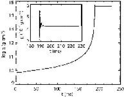
Figure 2: The central density is shown as a function of time for model R12B12X60.

Figure 2 shows the evolution of central density ($\rho_{c}$) for the period of $180~{}{\rm ms}\,\leq\,t\,\leq\,230~{}{\rm ms}$. The central density reaches its maximum, $5.49\times 10^{14}$ g cm^-3, at $t\,=\,189.05$ ms as well as in model R0B0. The period of dynamical collapse is a little longer and the maximum density is a little lower. The rotation and magnetic field delays the collapse a little as has been shown in earlier simulations. The PNS is only slightly flattened by rotation.

At $t\,=\,190.04$ ms (slightly after the bounce), the PNS has angular velocity of $\Omega_{c}\,=\,6.02\times 10^{3}~{}{\rm s}^{-1}$ and magnetic field of $B_{c}\,=\,7.56\times 10^{15}~{}{\rm G}$ at the center. The angular velocity and magnetic field increase by a factor of $5.0\times 10^{3}$ and $3.8\times 10^{3}$, respectively, from the initial values, while the density increases by a factor of $6.1\times 10^{4}$. These enhancements are consistent with the conservation of the specific angular momentum and magnetic flux, since the collapse is almost spherical. The angular velocity and magnetic field increase in proportion to $\rho^{2/3}$ when the collapse is spherical. The rotation axis changes little. At this stage the centrifugal force is only 3 % of the gravity at the center of the PNS. The magnetic force is much weaker than the gravity and than the centrifugal force.

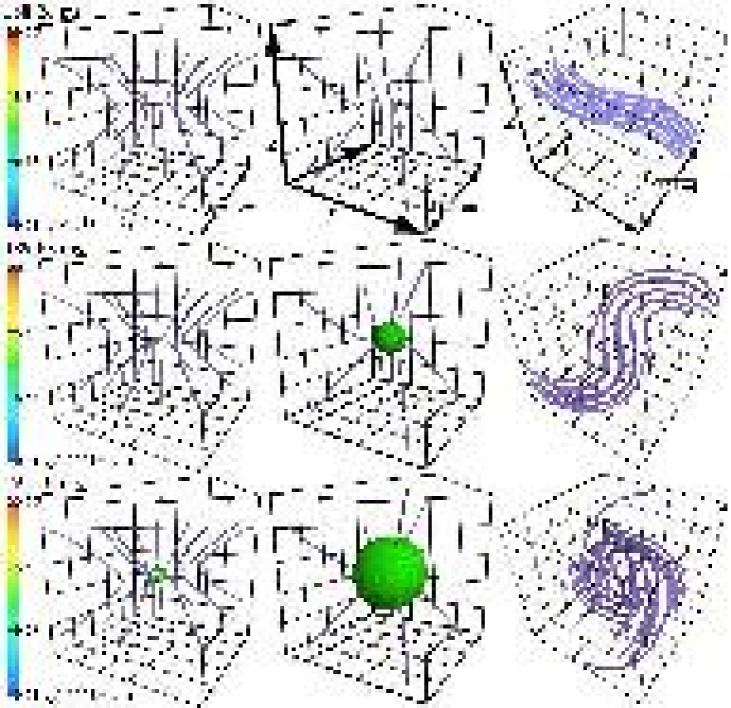
Figure 3: The evolution of magnetic field in model R12B12X60. Each panel denotes the magnetic field lines (purple lines) and the isovelocity surface of radial velocity, $v_{r}$, at a given stage. The panels are arranged in the time sequence from top to bottom. The top panels denote the stage of $t$ = 188.28 ms, while the bottom ones do that of $t$ = 191.10 ms. The left panels denote the central cube of (1691 km)³, while the central and right ones do the zoom-up views of of (423 km)³ and (26 km)³, respectively. The left color bars denote the radial velocity on the surface of the cubes in the unit of 10³ km s^-1.

The change in the magnetic field is illustrated in Figure 3. The magnetic field is almost radial near the end of dynamical collapse as shown in the top panels, in which the purple lines denote the magnetic field lines at $t$ = 188.28 ms by bird’s eye view. This is because the magnetic field is stretched in the radial direction by the dynamical collapse. The radial component of the magnetic field, $B_{r}$, is positive in the upper half of $z\,>\,0$, while it is negative in the lower half. Thus the split monopole is a good approximation to the magnetic field at this stage.

The magnetic field is twisted by the spin of PNS as shown in the middle and bottom panels of Figure 3. The azimuthal component of the magnetic field is amplified to have a large amplitude in the upper atmosphere of the PNS ($9~{}{\rm km}\,\lesssim\,r\,\lesssim\,14~{}{\rm km}$). The increase in the azimuthal component decreases the plasma beta down to $\beta\,\equiv\,P_{\rm gas}/P_{\rm mag}\,\simeq\,0.03$. The azimuthal component of the magnetic field is small inside the PNS, since the angular velocity is nearly constant. It is also small in the region very far from the center ($r\,>\,60~{}{\rm km}$) since the angular velocity is very small. It is also small near the rotation axis. Thus the region of strong twisted magnetic field has a torus-shape.

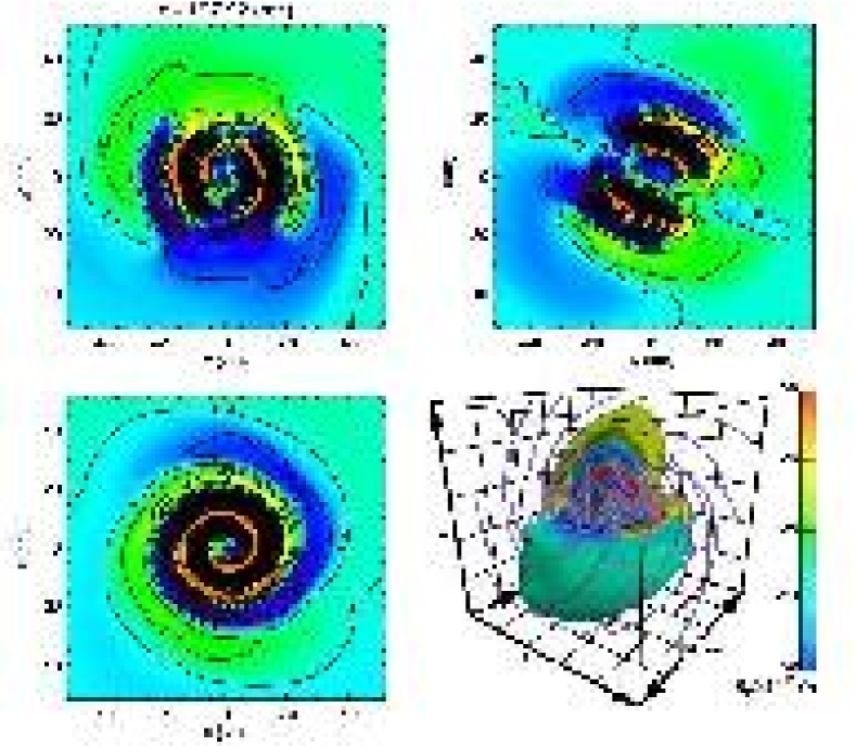
Figure 4: Structure of magnetic torus is shown by three cross sections and a bird’s eye view. The color denotes the azimuthal component of magnetic field, $B_{\varphi}\,=\,\mbox{\boldmath$e$}_{\varphi}\cdot\mbox{\boldmath$B$}$ on the planes of $x\,=\,0$ (upper left), $y\,=\,0$ (upper right), and $z\,=\,0$ (lower right) at $t\,=\,197.92$ ms. The contours denote $B_{\varphi}$ in unit of $10^{15}$ G. The lower right panels magnetic field lines (purple) and isosurface of $B_{\varphi}$ by the bird’s eye view.

The structure of twisted magnetic field is different from that in an aligned rotator. When the initial magnetic field is aligned to initial rotation axis, the twisted magnetic field has opposite directions in the upper and lower halves. The azimuthal component vanishes on the equator of rotation and has a large amplitude in the upper and lower tori. The magnetic field is uni-directional in each torus. In case of oblique rotator, however, these tori are mixed into a torus, in which the azimuthal component of magnetic field is bi-directional as a result. Figure 4 shows the distribution of toroidal component of magnetic field, $B_{\varphi}\,=\,(\mbox{\boldmath$e$}_{\varphi}\cdot\mbox{\boldmath$B$})$, at $t\,=\,197.92~{}{\rm ms}$, where $\mbox{\boldmath$e$}_{\varphi}\,=\,\mbox{\boldmath$e$}_{\Omega}\times\mbox{\boldmath$r$}/|\mbox{\boldmath$e$}_{\Omega}\times\mbox{\boldmath$r$}|$ ($\mbox{\boldmath$e$}_{\Omega}$ denotes the unit vector along the initial rotation axis and heads upper left in Figure 4). The toroidal component changes its sign alternately with an average interval of $\sim 5$ km.

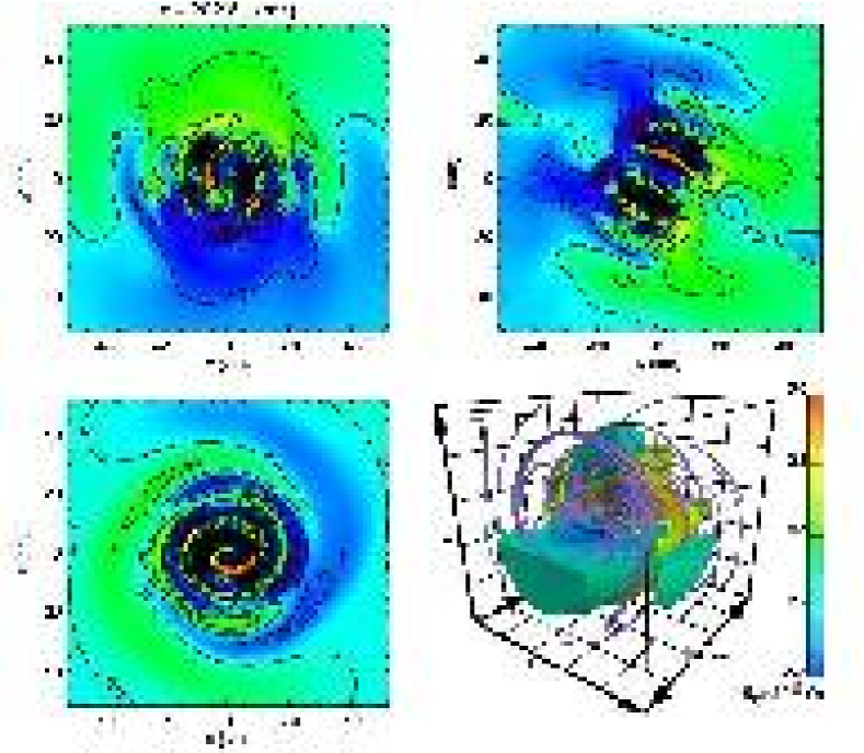
Figure 5: The same as Fig. 4 but for the stage at $t$ =202.81 ms.

Figure 5 is the same Figure 4 but for the 4.89 ms later stage. The magnetic field is wound more tightly inside the PNS and the toroidal component has extended outward.

A similar magnetic field is obtained semi-analytically as a model of pulsar magnetosphere by Bogovalov (1999). He approximated the initial magnetic field by split-monopole one and considered oblique rotation. As shown in his Figure 4, the toroidal component changes its sign with a regular interval in his pulsar wind solution. His idealized magnetic configuration is realized in our simulation. The magnetic multi-layers is inevitably formed when the initial magnetic field is split-monopole-like and inclined with respect to the rotation axis.

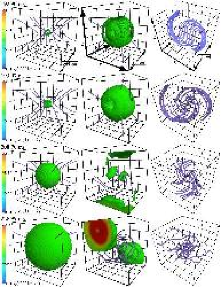
Figure 6: The same as Fig. 3 but for later stages of $t$ = 192.90 ms, 193.97 ms, 208.70 ms, and 228.99 ms.

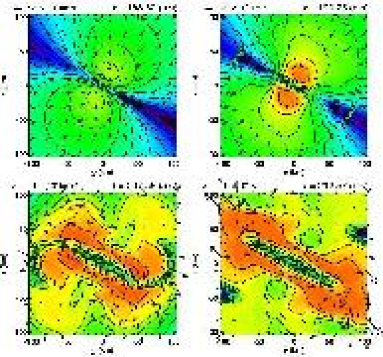
Figure 7: The evolution of rotation velocity. Each panel denotes the distribution of $\log\,v_{\varphi}$ (km s^-1) around the initial rotation axis in the cross section $x\,=\,0$ in model R12B12X60 by color and contours. The arrows denote the velocity within the plane. They denote the stages at $t$ = 188.52, 190.75, 207.56, and 212.96 ms.

Figure 6 shows later evolution of the magnetic field. The torus of twisted magnetic field expands slowly and bipolar jets are launched along the rotation axis. The jet reaches $r\,=\,400~{}{\rm km}$ at the last stage of computation ($t\,=\,228.99~{}{\rm ms}$). The jet velocity exceeds $3\times 10^{4}$ km s^-1. The jets are driven mainly by the magneto-centrifugal mechanism of Blandford & Payne (1982). Figure 7 shows the evolution of rotation velocity around the initial rotation axis. The rotation is nearly rigid in the sphere of $r\,\lesssim\,10~{}{\rm km}$ just before the bounce ($t$ = 188.52 ms). The rotation velocity increases up to $\sim\,5\times 10^{9}$ km s^-1 by the magnetic torque near the rotation axis. The magneto-centrifugal force is strong enough to drive jets. Although the centrifugal force is perpendicular to the rotation axis, the component perpendicular to the magnetic field is cancelled by the strong magnetic force. Thus the gas is accelerated along the poloidal magnetic field, i.e., along the rotation axis by the Blandford-Payne mechanism.

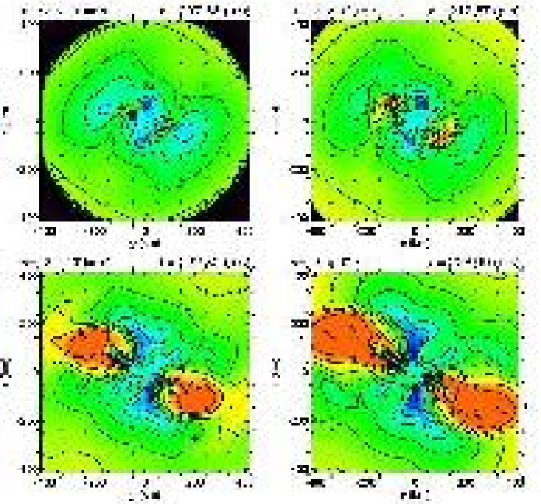
Figure 8: The radial velocity ($v_{r}$) distribution is denoted by color and contours for the stages at $t$ = 207.56, 212.57, 222.80, and 228.99 ms in model R12B12X60. The numbers attached to the contours denote $v_{r}$ in unit of $10^{4}$ km s^-1. The arrows denote the velocity within the cross section.

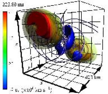
Figure 9: Jets and fast radial inflows in model R12B12X60. The panel denotes the central cube of $(423~{}{\rm km})^{3}$ at $t$ = 222.80 ms by bird’s eye view. The magnetic field lines are denoted by the purple lines, while the radial velocity is denoted by the isosurfaces. The blue denotes the fast radial inflow ($v_{r}\leq-1.0\times 10^{4}$ km s^-1), while the others do jets ($v_{r}\geq 2.0\times 10^{4}$ km s^-1). The color bar is for the radial velocity distribution on the cube surfaces.

The increase in the radial velocity follows that in the rotation velocity. The acceleration of jets are shown in Figure 8. The radial velocity is still low at the stage shown in the upper left panel ($t$ = 207.56 ms). The high velocity jets emerge not from the PNS surface but from the upper layer of $r\,\simeq\,60$ km. The mass flux through the sphere of $r\,=\,300$ km is $\dot{M}$ = 0.0, 7.64, 5.43, 5.58, 3.75, 2.07 M_⊙ s^-1 at $t$ = 190.75, 207.56, 212.96, 222.80, and 228.99 ms, respectively. Figure 9 shows the jets by bird’s eye view at the stage of $t$ = 222.80 ms. The jets are bipolar and well collimated.

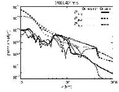
Figure 10: Pressure distribution is shown for the stage at $t$ = 208.42 ms. The solid curves denote the magnetic pressure, $|\mbox{\boldmath$B$}|^{2}/8\pi$, while the dashed curves denote the gas pressure. The dash-dotted curves denote the dynamical pressure, $\rho|\mbox{\boldmath$v$}|^{2}$. The thick curves are for the values on the initial rotation axis while the thin curves for those on equator.

The magnetic force is comparable to the gas pressure in the jets. Figure 10 denotes the magnetic pressure distribution at $t$ = 208.42 ms. The thick solid curve denotes the magnetic pressure, $|\mbox{\boldmath$B$}|^{2}/8\pi$, along the initial rotation axis, while thin solid curve does that on the equator. The magnetic pressure is enhanced by winding in the range $50~{}{\rm km}\,\lesssim\,r\,\lesssim\,100~{}{\rm km}$ on the axis. Also the dynamical pressure (rotation energy) is enhanced in the same region. Since these energies are large enough, the jets will extend outwards even if the prompt shock has stalled around $r\,\simeq\,100$ km.

We computed the energy of magnetic field, rotation and jets to evaluate the efficiency of energy conversion. The magnetic energy distribution is evaluated by

$$\varepsilon_{\rm mag}(r,~{}t)\;\equiv\;\int\int r^{3}\,\frac{|\mbox{\boldmath$B$}\,(r,~{}\theta,~{}\varphi,~{}t)|^{2}}{8\pi}\,\sin\theta\,d\theta\,d\varphi\,,$$ (20)

i.e., the energy stored in a unit logarithmic radial distance. The total magnetic energy is expressed as

$$E_{\rm mag}(t)\;=\;\int\,\varepsilon_{\rm mag}(r,~{}t)\,d\ln r\,.$$ (21)

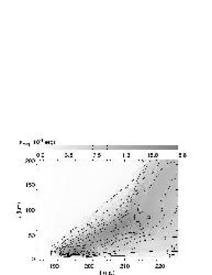
Figure 11: The magnetic energy stored in a unit logarithmic radial distance, $\varepsilon_{\rm mag}(r,~{}t)$, is shown by darkness. The contour levels are set to be $\Delta\varepsilon_{\rm mag}=10^{48}$ erg. The abscissa is the time ($t$) while the ordinate is radial distance ($r$).

Figure 11 shows that the magnetic energy has a sharp peak of $\varepsilon_{\rm mag}=1.88\times 10^{49}$ erg in the layer of $r\,\simeq\,18~{}{\rm km}$ at $t~{}\simeq~{}196~{}{\rm ms}$. The peak of the magnetic energy shifts outward at the apparent radial velocity of $3\times 10^{3}$ km s^-1, which coincides with the Alfvén velocity. The peak declines beyond $r\,\gtrsim\,80$ km.

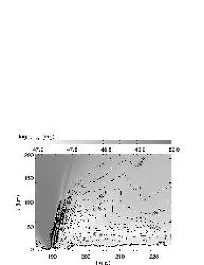
Figure 12: The same as Fig. 11 but for the radial kinetic energy, $\varepsilon_{\rm kin,rad}$.

Figure 12 is the same as Figure 11 but for the radial kinetic energy stored in a unit logarithmic radial distance,

$$\varepsilon_{{\rm kin,rad}}(r,~{}t)\;\equiv\;\int\int r^{3}\,\frac{\rho\,(r,~{}\theta,~{}\varphi)\,|\mbox{\boldmath$n$}\cdot\mbox{\boldmath$v$}\,(r,~{}\theta,~{}\varphi,~{}t)|^{2}}{2}\,\sin\theta\,d\theta\,d\varphi\,,$$ (22)

where $\mbox{\boldmath$n$}\,\equiv\,\mbox{\boldmath$r$}/|\mbox{\boldmath$r$}|$ denotes the unit radial vector. In the region far from the center, the dynamical collapse dominates in the radial kinetic energy. After the bounce ($t\,>\,189.72~{}{\rm ms}$), the prompt shock propagates and the region of the dynamical collapse retreats. (The propagation of prompt shock is mainly due to neglect of neutrino loss. If we had incorporated the neutrino cooling, the prompt shock should have stalled around 100-200 km.) The radial kinetic energy is small in the region of $r\,\lesssim\,60~{}{\rm km}$ after the bounce. The bipolar jets increase the radial kinetic energy in the region of $r\,\gtrsim\,80~{}{\rm km}$. The rise in $\varepsilon_{{\rm kin,rad}}$ coincides with the decline in $\varepsilon_{\rm mag}$. This is an evidence that the jets are accelerated by magnetic force.

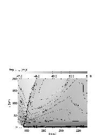
Figure 13: The same as Fig. 11 but for the rotational energy, $\varepsilon_{{\rm kin,rot}}$.

Figure 13 shows the distribution of the kinetic energy stored in a unit logarithmic radial distance,

$$\varepsilon_{{\rm kin,rot}}(r,~{}t)\;\equiv\;\int\int r^{3}\,\frac{\rho\,(r,~{}\theta,~{}\varphi)\,|\mbox{\boldmath$n$}\times\mbox{\boldmath$v$}\,(r,~{}\theta,~{}\varphi,~{}t)|^{2}}{2}\,\sin\theta\,d\theta\,d\varphi\,.$$ (23)

A large amount of rotation energy is stored in the region of $10~{}{\rm km}\,\lesssim\,r\,\lesssim\,20~{}{\rm km}$. Only a small fraction of it is converted into the energy of twisted magnetic field and eventually into the energy of jets.

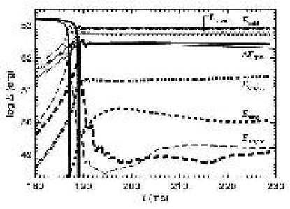
Figure 14: The evolution of energy in model R12B12X60. Each thick curve denotes a component of the energy stored in the sphere of $r\,\leq\,63$ km. The thin curves denote those in model R0B0.

Figure 14 shows the evolution of energy stored in the volume of $r\,\leq\,63~{}{\rm km}$ for each component. The gravitational energy, which is evaluated to be

$$E_{\rm grav}\;=-\;\int_{0}^{63~{}{\rm km}}\,\frac{|\mbox{\boldmath$g$}|^{2}}{8\pi G}\,dV\,,$$ (24)

is the most dominant and the internal energy is comparable. The thick solid curve denotes, $\Delta E_{\rm grav}\,\equiv\,E_{\rm grav}\,-\,E_{\rm grav,\min}$, the difference from the minimum value, i.e., the gravitational energy at the stage of the maximum central density (bounce). The rotation energy is order of magnitude smaller than them and the magnetic energy is further smaller. Only a small fraction of the rotation energy is converted into magnetic energy, which is mostly due to toroidal magnetic field. The energy available for jet ejection is limited by the conversion factor from rotation energy to magnetic energy. The radial kinetic energy is only of the order of $\sim 10^{49}$ erg in the period $t\,\geq\,195$ ms since the prompt shock and jets are outside the region. For comparison we show the evolution of the energy stored in model R0B0 by thin curves.

Note that the rotational energy available is much smaller than those in Obergaulinger et al. (2006a). Since the initial rotation energy was much larger in their simulation, the PNS shrunk appreciably after liberating the angular momentum through magnetic braking. Even if the rotation energy were released completely in our model, the PNS would not shrink appreciably.

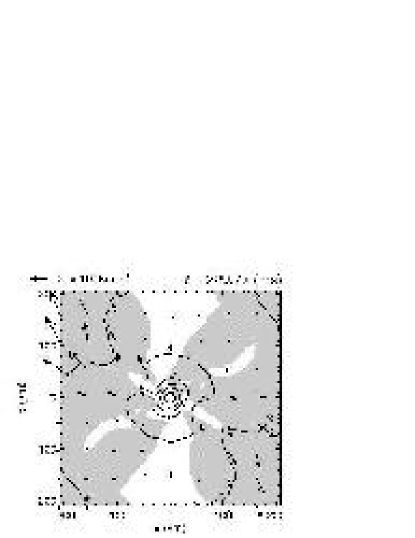
Figure 15: The velocity distribution are denoted by the arrows on the plane of $x\,=\,0$ at $t\,=\,229.77~{}{\rm ms}$. The scale is shown on the upper left corner. The darkness denotes the region of positive $v_{r}$ while the contours denote isodensity curves and labeled by $\log\,\rho$.

When the fast jets are ejected along the initial rotation axis, two other radial flows are observed. Figure 15 shows the velocity distribution on the plane of $x\,=\,0$ at $t\,=\,229.77~{}{\rm ms}$. One is slow outflow extending near the equator of initial rotation. The outflow velocity is approximately $2.5\times 10^{4}~{}{\rm km}~{}{\rm s}^{-1}$. The other is fast radial inflow located between the jets and equatorial outflow. The inflow is less dense and its dynamical pressure is much smaller than the magnetic pressure.

As shown earlier, the bipolar jets emanate from $r\,\simeq\,60~{}{\rm km}$. In the outer region of $r\,\gtrsim\,60~{}{\rm km}$, the density is lower than $\rho\,\lesssim\,10^{10}~{}{\rm gm}~{}{\rm cm}^{-3}$ (see Figure 1 for the average density distribution in model R0B0) and hence the Alfvén velocity is high. In other words, the magnetic force dominates over the pressure force. The centrifugal force is also important in the outer region. If the magnetic field corotates with the PNS, the rotation velocity is evaluated to be

$$v_{\varphi}\;=\;3.6\times 10^{4}\,\left(\frac{\Omega_{c}}{6\times 10^{3}~{}{\rm s}^{-1}}\right)\,\left(\frac{\varpi}{60~{}{\rm km}}\right)\,{\rm~{}km~{}s^{-1}},$$ (25)

where $\varpi$ denotes the distance from the rotation axis. The rotation velocity is close to the Keplerian velocity,

$$v_{K} = \sqrt{\frac{GM}{r}}$$ (26)

$$= 4.70\times 10^{4}\,\left(\frac{M}{1~{}{\rm M}_{\odot}}\right)^{1/2}\left(\frac{r}{60~{}{\rm km}}\right)^{-1/2}\,{\rm~{}km~{}s^{-1}}$$ (27)

where $M$ and $r$ denote the PNS mass and the distance from the center, respectively. In other words, the centrifugal force is comparable with the gravity. Thus the foot point of MHD jets coincides with the inner edge of the region in which the magnetic and centrifugal forces are dominant over the gravity.

As shown in Figure 4 the twisted magnetic field are ordered and has no structures suggesting development of magneto-rotational instability (MRI; see e.g., Akiyama et al., 2003). However, this is likely due to limited spatial resolution and will not exclude the possibility of MRI. Etienne, Liu, & Shapiro (2006) demonstrated that MRI can not grow unless the cell width is shorter than a tenth wavelength of the fastest growing mode. Since the wavelength is evaluated to be

$$\lambda_{\rm MRI} \approx 4\pi\,\left(r\frac{d\Omega^{2}}{dr}\right)^{-1/2}\,\frac{B}{\sqrt{4\pi\rho}}$$ (28)

$$= 1.18\,\left[\frac{d\Omega^{2}/d\ln r}{\left(3000~{}{\rm s}^{-1}\right)^{2}}\right]^{-1/2}\,\left(\frac{B}{10^{15}~{}{\rm G}}\right)\,\left(\frac{\rho}{10^{14}~{}{\rm g}~{}{\rm cm}^{-3}}\right)^{-1/2}\,{\rm km}\,,$$ (29)

we need the spatial resolution of $\sim~{}120$ m to observe MRI.

3.3 Dependence on $B_{0}$

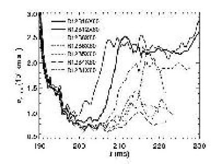
Figure 16: The maximum radial velocity is shown as a function of time for various models having different initial magnetic field.

To examine the effect of initial magnetic field we made 6 models by changing only $B_{0}$ from model R12B12X60. Figure 16 shows the maximum radial velocity ($v_{r,\max}$) as a function of time. It declines sharply in the period of $t\leq 195$ ms, since the prompt shock wave slows down. The early decline is delayed when $B_{0}$ is larger. The delay is, however, smaller than 1 ms since the magnetic energy is much smaller than the gravitational energy at the PNS formation. See Table 3 for comparison of models at the bounce.

The late rise in $v_{r,\max}$, i.e., the launch of MHD jets depends strongly on $B_{0}$. When $B_{0}$ is larger, the radial velocity rises earlier and stays at a high level. When $B_{0}$ is smaller than $1.0\times 10^{12}~{}{\rm G}$, the radial velocity increases late but decreases soon before reaching a high level.

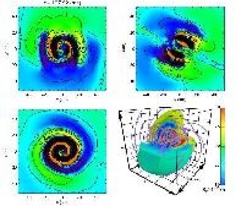
Figure 17: The same as Fig. 4 but for model R12B16X60.

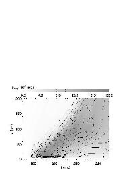
Figure 18: The same as Fig. 11 but for model R12B16X60.

When $B_{0}$ is large, the magnetic field is less tightly twisted since the twisted component drifts upward faster. Figure 17 is the same as Figure 4 but for model R12B16X60, in which $B_{0}$ is $4/3$ times larger than in the standard model R12B12X60. The toroidal component, $B_{\varphi}$, changes its sign with a longer average interval of 5–6 km on the average, while it does with an interval of 5 km in the standard model. At $t\,\simeq\,206~{}{\rm ms}$, the twisted magnetic field reaches $r\,=\,60~{}{\rm km}$ as shown in Figure 18 and the MHD jets initiate.

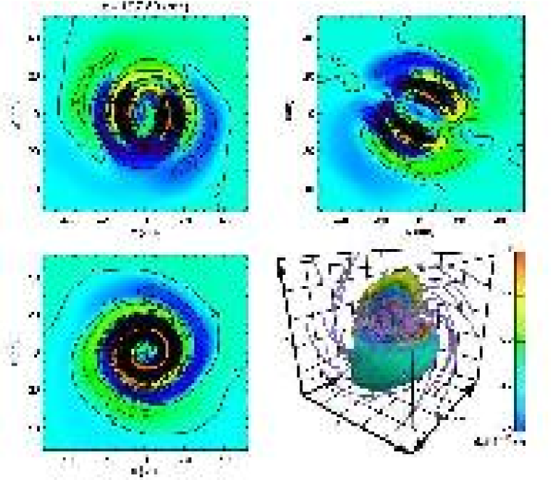
Figure 19: The same as Fig. 4 but for model R12B8X60.

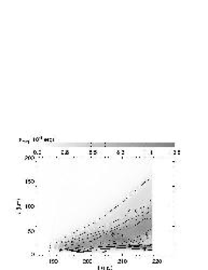
Figure 20: The same as Fig. 11 but for model R12B8X60.

On the other hand, the magnetic field is more tightly twisted when $B_{0}$ is smaller. Figure 19 is the same as Figure 4 but for model R12B8X60. The toroidal component, $B_{\varphi}$, changes its sign with a shorter interval of 3–4 km on the average. The twisted magnetic field rises up slowly and dwindles as shown in Figure 20. Accordingly the jets are launched but late and weak as shown in Figure 19, where the evolution of the maximum radial velocity, $v_{r,{\rm max}}$, is shown for various models having different $B_{0}$. The weakness of the jet is at least partly due to numerical diffusion. Remember that the spatial resolution is 0.826 km in the central cube of (53.0 km)³. Thus the numerical diffusion is appreciably large for the magnetic multi-layers since the typical interval is less than 10 km. The MHD jets would be more powerful if the numerical diffusion were suppressed.

See Table 4 to compare models at the final stages.

3.4 Dependence on $\Omega_{0}$

To examine the effect of initial rotation, we made 5 models by changing only $\Omega_{0}$ from model R12B12X60. All the models show qualitatively similar results. The differences are mainly quantitative.

The initial rotation is twice slower in model R6B12X60 than in model R12B12X60. Accordingly the PNS has twice lower angular velocity in model R6B12X60. The magnetic field is twisted by rotation also in model R6B12X60 but the toroidal component is weaker since the rotation is slower. The MHD jets are launched but at a little later epoch.

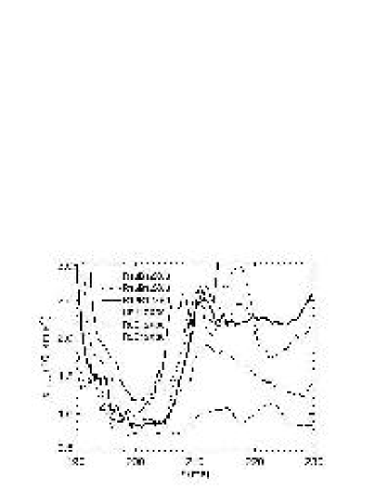
Figure 21: The same as Fig. 16 but various models having different initial angular velocity.

Figure 21 shows the evolution of the maximum radial velocity, $v_{r,\max}$, as a function of time for various models having different $\Omega_{0}$. The early decline in $v_{r,\max}$ is due to the deceleration of the prompt shock. The late rise in $v_{r,\max}$ is due to the launch of jets. When $\Omega_{0}$ is larger, the PNS is formed a little later and the jets are ejected a little earlier. The maximum radial velocity is slower when $\Omega_{0}$ is small.

The rotation energy of PNS is proportional to $\Omega_{0}^{2}$. It is $E_{\rm rot}\,=\,3.8\times 10^{52}~{}{\rm erg}$ in model R18B12X60 while it is $E_{\rm rot}\,=\,4.5\times 10^{51}~{}{\rm erg}$ in model R6B12X60. The energy of the jets, which is evaluated to be radial kinetic energy of outflowing gas, is also large in a model having a large $\Omega_{0}$.

3.5 Dependence on $\theta_{\Omega}$

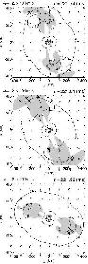
Figure 22: Comparison of radial velocity distribution between the models having different rotation axis ($\theta_{\Omega}$). The inclination angle is $\theta_{\Omega}~{}=~{}15^{\circ}$ (top), 30^∘ (middle), and 60^∘ (bottom), respectively. The arrows denote the velocity within the plane and the scale is shown on the top left of each panel. The radial velocity exceeds $v_{r}\,>\,5\times 10^{3}$ km s^-1 in the gray area. The contours denote the isodensity in the logarithmic scale and labeled by $\log\,\rho$.

To examine the effect of the initial inclination angle, we made 5 models by changing only $\theta_{\Omega}$ from model R12B12X60. Also in these models, the MHD jets are launched along the initial rotation axis (see Fig. 22).

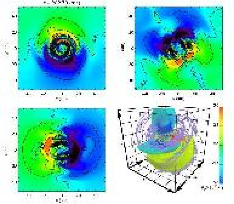
Figure 23: The same as Fig. 4 but for model R12B12X30 at $t$ =202.79 ms.

Figure 23 denotes the magnetic multi layer formed in model R12B12X30. The structure of magnetic multi layer depends on the inclination angle. When the inclination angle is smaller, it is confined in a narrower region around the equator. The radial interval of changing $B_{\varphi}$ depends little on the inclination angle.

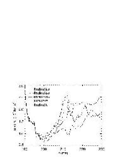
Figure 24: The same as Fig. 21 for various models having different initial inclination angle.

Figure 24 shows the evolution of the maximum radial velocity in these models. When $\theta_{\Omega}$ is larger, the maximum radial velocity rises earlier. In other words, the MHD jets are launched earlier when the rotation axis is inclined.

Although the rise is different, the maximum radial velocity reaches a certain value independently of the inclination angle. In other words, the terminal velocity is independent of the inclination angle, $\theta_{\Omega}$.

4 SUMMARY AND DISCUSSIONS

In this paper we have shown three dimensional MHD simulations of core collapse supernova for the first time. The numerical simulations explore the effects of inclined magnetic field and dependence on the initial magnetic field and rotation. We summarize the results and discuss the implications.

First we have confirmed that the MHD jets are ejected along the initial rotation axis. This is because the energy of rotation dominates over the magnetic energy at the moment of PNS formation. The magnetic force is too weak to change the rotation axis appreciably. Thus the magneto-centrifugal force accelerates gas along the initial rotation axis through the Blandford-Payne mechanism (see §3.2).

If the initial magnetic field were relatively strong, the rotation axis could change appreciably and also the jet direction could be different. A similar problem has been studied by Machida et al. (2006) for formation of a protostar. They considered collapse of a rotating molecular cloud core having an oblique magnetic field. They have found that the evolution of magnetic field and rotation axis depends on their relative strength. When the magnetic field is relatively strong, the magnetic braking acts to align the rotation axis with the magnetic field. Then the jets are ejected in the direction parallel to the initial magnetic field as shown first by Matsumoto & Tomisaka (2004).

The relative strength between rotation and magnetic field can be evaluated from the ratio of the angular velocity to the magnetic field, $\Omega/B$. The ratio remains nearly constant during the dynamical collapse since the free-fall timescale is very short. Both the angular velocity and magnetic field increase in proportion to the inverse square of core radius, since both the specific angular momentum and magnetic flux change little during the short dynamical collapse phase. Machida et al. (2006) proposed $\Omega_{0}/B_{0}\,>\,0.39~{}G^{1/2}c_{s}^{-1}$, as a criterion for the jets parallel to the initial rotation axis, where $c_{s}$ denotes the isothermal sound speed of the molecular cloud. Since the dynamics of collapse is similar, we can expect that the criterion holds also for core collapse supernova if we replace $c_{s}$ with an appropriate one. The criterion is rewritten as

$$\frac{\Omega_{0}\,c_{s}}{G^{1/2}\,B_{0}}\,>\,0.39\,.$$ (30)

The left hand side is evaluated to be

$$\frac{\Omega_{0}\,c_{s}}{G^{1/2}\,B_{0}} = 3.87\,\left(\frac{\Omega_{0}}{1~{}{\rm s}^{-1}}\right)\,\left(\frac{B_{0}}{10^{12}~{}{\rm G}}\right)^{-1}\,\left(\frac{c_{s}}{10^{4}\,{\rm km~{}s}^{-1}}\right)\,.$$ (31)

The criterion is consistent with our numerical simulations since the sound speed increases from $c_{s}\,=\,10^{4}~{}{\rm km~{}s}^{-1}$ to $10^{5}~{}{\rm km~{}s}^{-1}$ during the dynamical collapse. Although the assumed initial magnetic field is strong, it is still too weak to change the rotation axis unless the initial rotation is slow. Thus it is reasonable that the rotation is unchanged during the dynamical collapse since young pulsars are spinning fast.

Next we discuss the fate of magnetic multi-layers in which the toroidal magnetic field changes its direction with a regular interval. The magnetic multi-layers are a natural outcome of oblique rotation as shown in the previous section. These layers are potentially unstable against reconnection, although no features are seen for reconnection. It is also interesting to study the magnetic multi-layers with a higher spatial resolution. If the magnetic fields are reconnected, a large amount of the magnetic energy is released to lead an explosive process.

Next we discuss the lag between the bounce and jet ejection. When the initial magnetic field is weaker, the lag is longer as already shown in Ardeljan et al. (2004), Moiseenko et al. (2006), and Burrows et al. (2007). Our numerical simulations have suggested that the lag is related to the Alfvén transit time; the MHD jets are ejected when the twisted magnetic field reaches a certain radius, i.e., 60 km in our simulations. When the initial magnetic field is weak, the Alfvén transit time is longer and the magnetic field is amplified for a longer duration before the jet ejection. Since the larger amplification compensates for a weak seed field, almost the same amount of toroidal magnetic field is generated irrespectively of the initial magnetic field strength. This implies that strong MHD jets can be ejected even if the initial magnetic field is weak. If we could suppress numerical diffusion by improving resolution, strong MHD jets should be ejected also in model R12B5X60 and others having a weaker initial magnetic field as discussed in the previous section.

The Alfvén transit time is evaluated to be

$$\tau_{A} \equiv \int^{r_{j}}\frac{1}{v_{A}}\,dr$$ (32)

$$= \int^{r_{j}}\frac{\sqrt{4\pi\rho}}{B_{r}}\,dr\,,$$ (33)

where $r_{j}~{}$($\simeq$ 60 km) denotes the radius at the foot point of the jets. The radial magnetic field decreases in proportion to the inverse square of the radius ($\propto\,r^{-2}$) since the split monopole is a good approximation for the magnetic field at the epoch of PNS formation. The density decreases also roughly proportional to the inverse square of the radius ($\propto\,r^{-2}$) in the upper atmosphere of the PNS (see Figure 1). Accordingly the Alfvén velocity is roughly proportional to the radius, $v_{A}\,\propto\,r$ and the Alfvén transit time depends only weakly on $r_{j}$.

The above argument suggests a factor controlling the jet energy. The rotation energy of the PNS is much larger than the energy of jets. If the magnetic field is twisted for a longer period, i.e., if the Alfvén transit time is longer, a larger fraction of the rotation energy is converted into the jet energy. The Alfvén transit time can be extended if the magnetic field is twisted in a deep interior of the PNS.

Appendix A An Approximate Riemann Solution of the MHD Equations for Non-ideal Equation of State

For the approximate EOS of Takahara & Sato (1982), we have found a numerical flux which satisfies the property U of Roe (1981). The numerical flux is the same as that of Cargo & Gallice (1997) except for the correction term,

$$G\;=\;\overline{\varepsilon_{\rm cold}}\,+\,\overline{\rho}\,\frac{\Delta\varepsilon_{\rm cold}}{\Delta\rho}\,-\,\frac{1}{\gamma_{\rm t}\,-\,1}\,\frac{\Delta P_{\rm cold}}{\Delta\rho}\,$$ (A1)

where

$$\varepsilon_{\rm cold}\;=\;\int_{0}^{\rho}\frac{P_{\rm cold}}{\rho^{2}}\,d\rho\,.$$ (A2)

Here the bared symbols denote the Roe average while the symbols with the capital delta denote the differences between the two adjacent cells. The average specific enthalpy, $\bar{H}$, should be replaced with $\bar{H}\,-\,G$ in the computation of $a$ and $a_{*}$. Accordingly, the characteristic speeds propagating in the $x$-direction are evaluated to be

$$a^{2}\;=\;(\gamma_{t}\,-\,1)\,\left(\bar{H}\,-\,G\,-\,\frac{\bar{u}^{2}\,+\,\bar{v}^{2}\,+\,\bar{w}^{2}}{2}\,+\,\frac{B_{x}^{2}\,+\,\bar{B}_{y}^{2}\,+\,\bar{B}_{z}^{2}}{4\pi\bar{\rho}}\,-\,\delta{b}^{2}\right)\,,$$ (A3)

$$a_{*}^{2} = (\gamma_{t}\,-\,1)\,\left(\bar{H}\,-\,G\,-\,\frac{\bar{u}^{2}\,+\,\bar{v}^{2}\,+\,\bar{w}^{2}}{2}\,-\,\delta{b}^{2}\right)$$ (A4)

$$\;-\,(\gamma_{t}\,-\,2)\,\left(\frac{B_{x}^{2}\,+\,\bar{B}_{y}^{2}\,+\,\bar{B}_{z}^{2}}{4\pi\bar{\rho}}\right)\,,$$

where

$$\delta b^{2}\;=\;\frac{\gamma_{t}\,-\,1}{\gamma_{t}\,-\,2}\,\frac{\Delta B_{y}^{2}\,+\,\Delta B_{z}^{2}}{4\pi\,(\sqrt{\rho_{\rm L}}\,+\,\sqrt{\rho_{\rm R}})^{2}}\,.$$ (A5)

Here, $(u,\,v,\,w)$ and $(B_{x},\,B_{y},\,B_{z})$ denote the velocity and magnetic field, respectively. The symbols, $\Delta B_{y}$ and $\Delta B_{z}$, denote the difference between the two adjacent cells, while the symbols, $\rho_{\rm L}$ and $\rho_{\rm R}$ denote the density in the left hand side and that in the right hand side, respectively.

At the same time, the correction term $G$ should be added to the last component of the eigen vector of the entropy wave. This correction term is similar to that obtained by Nobuta & Hanawa (1999) for the numerical flux of hydrodynamical equations. Thus the right eigen vector for the entropy wave is expressed as,

$${}^{t}\mbox{\boldmath$r$}_{\rm entropy}\;=\;\left(1,\,\bar{u},\,\bar{v},\bar{w},\,0,\,0,\,0,\,\frac{\bar{u}^{2}\,+\,\bar{v}^{2}\,+\,\bar{w}^{2}}{2}\,+\,G\right)\,.$$ (A6)

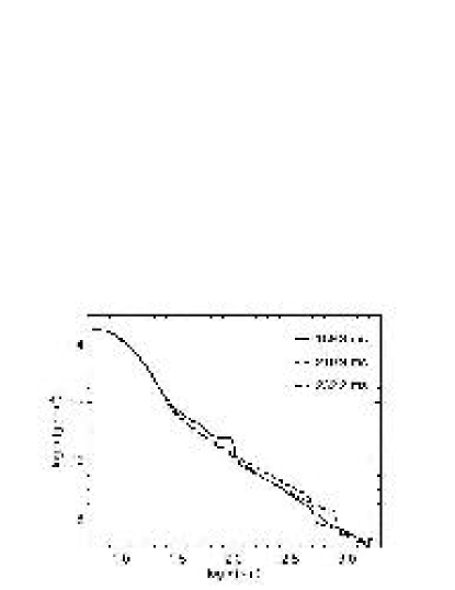
Figure 1: The angle averaged density, $\rho\,(r,~{}t)$, is shown as a function of $r$ for model R0B0.

Table 1: Model parameters for $P_{c}$. See Eq. 8.

$i$	$\rho_{i}$	$K_{i}$	$\gamma_{i}$
1	$4.0\times 10^{9}$	$1.767\times 10^{27}$	$4/3$
2	$1.0\times 10^{12}$	$2.446\times 10^{30}$	1.31
3	$2.8\times 10^{14}$	$4.481\times 10^{33}$	$4/3$
4	$1.0\times 10^{15}$	$1.080\times 10^{35}$	2.5

Table 2: Summary of the models. The initial gravitational energy is $W\,=\,-4.75\times 10^{51}$ erg in all the models. The models underlined are shown in detail in the main text.

model	$\Omega_{0}$	$E_{\rm kin}$	$\left|E_{\rm kin}/E_{\rm grav}\right|$	$B_{0}$	$E_{\rm mag}$	$\left|E_{\rm mag}/E_{\rm grav}\right|$	$\theta_{\Omega}$
	(s-1)	(erg)	(%)	(G)	(erg)	(%)
R0B0	0	0	0	0	0	0	$\cdots$
R12B12X60	1.2	2.2$\times 10^{48}$	$5.0\times 10^{-4}$	2.0$\times 10^{12}$	1.4$\times 10^{48}$	$2.9\times 10^{-4}$	60∘
R18B12X60	1.8	4.9$\times 10^{48}$	$1.1\times 10^{-3}$	2.0$\times 10^{12}$	1.4$\times 10^{48}$	$2.9\times 10^{-4}$	60∘
R15B12X60	1.8	3.4$\times 10^{48}$	$1.1\times 10^{-3}$	2.0$\times 10^{12}$	1.4$\times 10^{48}$	$2.9\times 10^{-4}$	60∘
R8B12X60	0.81	9.6$\times 10^{47}$	$2.0\times 10^{-4}$	2.0$\times 10^{12}$	1.4$\times 10^{48}$	$2.9\times 10^{-4}$	60∘
R6B12X60	0.61	5.4$\times 10^{47}$	$1.1\times 10^{-5}$	2.0$\times 10^{12}$	1.4$\times 10^{48}$	$2.9\times 10^{-4}$	60∘
R3B12X60	0.31	1.4$\times 10^{47}$	$2.0\times 10^{-4}$	2.0$\times 10^{12}$	1.4$\times 10^{48}$	$2.9\times 10^{-4}$	60∘
R12B16X60	1.2	2.2$\times 10^{48}$	$5.0\times 10^{-4}$	2.7$\times 10^{12}$	2.5$\times 10^{48}$	$5.8\times 10^{-4}$	60∘
R12B8X60	1.2	2.2$\times 10^{48}$	$5.0\times 10^{-4}$	1.3$\times 10^{12}$	6.2$\times 10^{47}$	$1.4\times 10^{-4}$	60∘
R12B6X60	1.2	2.2$\times 10^{48}$	$5.0\times 10^{-4}$	1.0$\times 10^{12}$	3.5$\times 10^{47}$	$8.1\times 10^{-5}$	60∘
R12B5X60	1.2	2.2$\times 10^{48}$	$5.0\times 10^{-4}$	8.4$\times 10^{11}$	2.4$\times 10^{47}$	$5.6\times 10^{-5}$	60∘
R12B4X60	1.2	2.2$\times 10^{48}$	$5.0\times 10^{-4}$	6.7$\times 10^{11}$	1.6$\times 10^{47}$	$3.6\times 10^{-5}$	60∘
R12B1X60	1.2	2.2$\times 10^{48}$	$5.0\times 10^{-4}$	1.7$\times 10^{11}$	9.7$\times 10^{45}$	$2.3\times 10^{-6}$	60∘
R12B12X30	1.2	2.2$\times 10^{48}$	$5.0\times 10^{-4}$	2.0$\times 10^{12}$	1.4$\times 10^{48}$	$2.9\times 10^{-4}$	30∘
R12B12X15	1.2	2.2$\times 10^{48}$	$5.0\times 10^{-4}$	2.0$\times 10^{12}$	1.4$\times 10^{48}$	$2.9\times 10^{-4}$	15∘
R12B12X7	1.2	2.2$\times 10^{48}$	$5.0\times 10^{-4}$	2.0$\times 10^{12}$	1.4$\times 10^{48}$	$2.9\times 10^{-4}$	7∘
R12B12X0	1.2	2.2$\times 10^{48}$	$5.0\times 10^{-4}$	2.0$\times 10^{12}$	1.4$\times 10^{48}$	$2.9\times 10^{-4}$	0∘

Table 3: Comparison of models at the bounce.

model	$t$	$T/\left|W\right|$	${\cal M}/\left|W\right|$	$T$	${\cal M}$	$\omega_{\rm max}$	$B_{\rm max}$
	(ms)	(%)	(%)	($10^{50}$ erg)	($10^{50}$ erg)	(kHz)	($10^{15}$ G)
R0B0	$191.9$	$0.5854$	0.000	$8.359$	0.000	$0.1421$	0.000
R12B12X60	$192.2$	$2.137$	$0.1002$	$30.46$	$1.428$	$29.97$	$17.96$
R18B12X60	$192.2$	$4.315$	$0.07094$	$57.21$	$0.9405$	$38.21$	$13.48$
R15B12X60	$194.1$	$2.703$	$0.1679$	$37.72$	$2.344$	$38.44$	$21.25$
R8B12X60	$191.9$	$1.309$	$0.07185$	$18.61$	$1.021$	$26.50$	$16.08$
R6B12X60	$193.1$	$0.9306$	$0.07122$	$13.24$	$1.013$	$16.72$	$18.46$
R3B12X60	$193.2$	$0.6340$	$0.04088$	$9.019$	$0.5815$	$6.329$	$18.04$
R12B16X60	$192.7$	$2.033$	$0.1721$	$28.91$	$2.447$	$28.20$	$23.09$
R12B8X60	$192.3$	$2.150$	$0.05520$	$30.53$	$0.7840$	$28.39$	$13.41$
R12B6X60	$192.6$	$2.022$	$0.1000$	$28.17$	$1.394$	$7.656$	$16.68$
R12B5X60	$192.3$	$2.180$	$0.02334$	$30.96$	$0.3314$	$27.82$	$9.320$
R12B4X60	$220.7$	$2.887$	$0.01407$	$41.06$	$0.2001$	$31.03$	$9.416$
R12B1X60	$192.5$	$2.127$	$0.08790$	$30.23$	$1.249$	$35.31$	$16.50$
R12B12X30	$194.9$	$1.986$	$0.1384$	$27.98$	$1.950$	$42.41$	$16.26$
R12B12X15	$194.9$	$1.981$	$0.1423$	$27.91$	$2.005$	$41.17$	$16.83$
R12B12X7	$192.7$	$2.036$	$0.03528$	$28.22$	$0.4889$	$43.35$	$6.467$

Table 4: Comparison of models at the final stage.

model	$t$	$T/\left|W\right|$	${\cal M}/\left|W\right|$	$T$	${\cal M}$	$\Delta E_{\rm grav}$	$\omega_{\rm max}$	$B_{\rm max}$
	(ms)	(%)	(%)	($10^{50}$ erg)	($10^{50}$ erg)	($10^{50}$ erg)	(kHz)	($10^{15}$ G)
R0B0	$232.2$	$0.1552$	0.000	$2.312$	0.000	$61.53$	$5.123$	0.000
R12B12X60	$229.0$	$2.277$	$0.1835$	$32.44$	$2.615$	$1.002$	$27.80$	$12.80$
R18B12X60	$215.8$	$3.497$	$0.1955$	$48.38$	$2.705$	$57.54$	$32.85$	$15.89$
R15B12X60	$224.4$	$2.988$	$0.2084$	$42.11$	$2.937$	$13.59$	$32.59$	$14.21$
R8B12X60	$228.7$	$1.200$	$0.1547$	$17.33$	$2.235$	$23.50$	$19.85$	$13.99$
R6B12X60	$231.9$	$0.7440$	$0.1066$	$10.94$	$1.568$	$47.14$	$12.32$	$14.89$
R3B12X60	$233.2$	$0.2592$	$0.06470$	$3.853$	$0.9616$	$63.81$	$5.220$	$11.56$
R12B16X60	$230.5$	$2.010$	$0.2382$	$28.77$	$3.409$	$8.921$	$24.99$	$12.74$
R12B8X60	$227.7$	$2.514$	$0.1548$	$35.67$	$2.197$	$1.261$	$38.35$	$13.37$
R12B6X60	$224.9$	$1.773$	$0.1817$	$23.26$	$2.383$	$81.68$	$12.02$	$12.99$
R12B5X60	$220.5$	$2.550$	$0.1770$	$35.96$	$2.495$	$9.983$	$29.23$	$17.35$
R12B4X60	$223.7$	$3.011$	$0.01702$	$43.08$	$0.2435$	$7.955$	$31.27$	$11.05$
R12B1X60	$217.6$	$1.933$	$0.2232$	$27.24$	$3.145$	$12.26$	$38.46$	$15.85$
R12B12X30	$230.6$	$2.208$	$0.3719$	$30.72$	$5.174$	$17.36$	$43.41$	$14.15$
R12B12X15	$209.0$	$1.712$	$0.3392$	$23.83$	$4.722$	$16.61$	$34.29$	$28.97$
R12B12X7	$231.8$	$1.864$	$0.2876$	$23.79$	$3.669$	$110.0$	$37.51$	$34.89$

References

- Akiyama et al. (2003) Akiyama, S., Wheeler, J.C., Meier, D. L., & Lichtenstadt, I., 2003, ApJ, 584, 954
- Ardeljan et al. (2004) Ardeljan, N. V., Bisnovatyi-Kogan, G. S., Kosmachevskii, K. V., & Moiseenko, S. G. 2004, Astrophys., 47, 1
- Balsara (2001) Balsara, D. S., 2001, J. Comput. Phys., 174, 614
- Balsara & Spicer (1999) Balsara, D. S., & Spicer, D. S., 1999, J. Comput. Phys., 149, 270
- Blandford & Payne (1982) Blandford, R. D., Payne, D. G. 1982, MNRAS, 199, 838
- Blondin et al. (2003) Blondin, J. M., Mezzacappa, A., & Demarino, C. 2003, ApJ, 584, 971
- Blondin & Mezzacappa (2007) Blondin, J. M., Mezzacappa, A. 2007, Nature, 445, 58
- Bogovalov (1999) Bogovalov, S. V. 1999, A&A, 349, 1017
- Buras et al. (2007) Buras, R., Janka, H.-Th., Rampp, M., & Kifonidis, K. A&A, 457, 281
- Burrows et al. (2006) Burrows, A., Livne, E., Dessart, L., Ott, C. D., & Murphy, J. 2006, 640, 878
- Burrows et al. (2007) Burrows, A., Dessart, L., Livne, E., Ott, C., & Murphy, J. 2007, ApJ, 664, 416
- Cargo & Gallice (1997) Cargo, P. & Gallice, G. 1997, J. Comput. Phys., 136, 446
- Etienne, Liu, & Shapiro (2006) Etienne, Z. B., Liu, Y. T., & Shapiro, S. L. 2006, Phys. Rev. D, 74 044030
- Evans & Hawley (1998) Evans, C., & Hawley, J. F., 1988, ApJ, 332, 659
- Hanawa et al. (2007) Hanawa, T., Mikami, H., Matsumoto, T. 2007, private communication (submitted to the Journal of Computational Physics in April 2007)
- Heger, Woosley, & Spruit (2005) Heger, A., Woosley, S. E., & Spruit, H. C. 2005, ApJ, 623, 350
- Hwang et al. (2004) Hwang, U. et al. 2004, ApJ, 615, L117
- LeBlanc & Wilson (1970) LeBlanc, J. M., & Wilson, J. R. 1970, ApJ, 161, 541
- Leonard et al. (2006) Leonard, D. C. et al. 2006, Nature, 440, 505
- Machida et al. (2006) Machida, M. N., Matsumoto, T., Hanawa, T., & Tomisaka, K. 2006, ApJ, 645, 1227
- Matsumoto & Hanawa (2003) Matsumoto, T., & Hanawa, T. 2003, ApJ, 595, 913
- Matsumoto & Tomisaka (2004) Matsumoto, T., & Tomisaka, K. 2004, ApJ, 616, 266
- Moiseenko et al. (2006) Moiseenko, S. G., Bisnovatyi-Kogan, G. S., & Ardeljan, N. V. 2006, MNRAS, 370, 501
- Nobuta & Hanawa (1999) Nobuta, K., & Hanawa, T. 1999, ApJ, 510, 614
- Obergaulinger et al. (2006a) Obergaulinger, M., Aloy, M. A., & Müller 2006, A&A, 450, 1170
- Obergaulinger et al. (2006b) Obergaulinger, M., Aloy, M. A., Dimmelmeir, H., & Müller 2006, A&A, 457, 209
- Roe (1981) Roe, P. L. J. Comput. Phys., 43, 357
- Sawai (2005) Sawai, H., Kotake, K., & Yamada, S. 2005, ApJ, 631, 446
- Shibata et al. (2006) Shibata, M., Liu, Y. T., Shapiro, S. L., & Stephens, B. C. 2006, Phys. Rev. D, 74, 104026
- Sumiyoshi et al. (2005) Sumiyoshi, K., Yamada, S., Suzuki, H., Shen, H., Chiba, S., & Toki, H. 2005, ApJ, 629, 922
- Takahara & Sato (1982) Takahara, M., Sato, K. 1982, Prog. Theor. Phys., 68, 79
- Takiwaki et al. (2004) Takiwaki, T., Kotake, K., Nagataki, S., & Sato, K. 2004, ApJ, 616, 1086
- Wang et al. (2003) Wang, L., Baade, D., Höfligh, P., & Wheeler, J. C. 2003, ApJ, 592, 457
- Wang et al. (2002) Wang, L. et al. 2002, ApJ, 579, 671
- Woosley et al. (2002) Woosley, S. E., Heger, A., Weaver, T. A., 2002, Rev. Mod. Phys., 74, 1015
- Yamada & Sawai (2004) Yamada, S., & Sawai, H. 2004, ApJ, 608, 907