AC magnetization transport and power absorption in non-itinerant spin chains

Abstract

We investigate the ac transport of magnetization in non-itinerant quantum systems such as spin chains described by the XXZ Hamiltonian. Using linear response theory, we calculate the ac magnetization current and the power absorption of such magnetic systems. Remarkably, the difference in the exchange interaction of the spin chain itself and the bulk magnets (i.e. the magnetization reservoirs), to which the spin chain is coupled, strongly influences the absorbed power of the system. This feature can be used in future spintronic devices to control power dissipation. Our analysis allows to make quantitative predictions about the power absorption and we show that magnetic systems are superior to their electronic counter parts.

Power dissipation is one of the most important limitations of state-of-the-art electronic systems. The same is true for spintronic devices in which spin transport is accompanied by charge transport. In non-itinerant quantum systems, the dissipation problem is reduced since true magnetization transport generates typically much less power than charge currents hall2006 ; ovchi2008 . This is one of the main reasons for putting so much hope and effort into spin-based devices for future applications wolf2001 ; awschalom2002 ; awschalom2007 .

Here, we analyze non-itinerant quantum systems described by a spin Hamiltonian in which ac magnetization transport occurs via magnons or spinons (without the transport of charge). In Ref. meier2003 , the spin conductance of such a device has been derived with a particular focus on the role of the magnetization reservoirs to which a one-dimensional spin chain is attached. We generalize this theory to the response to an ac magnetization source. This allows us to directly calculate (and thus estimate) the power absorption of such magnetic systems at a given driving frequency $\omega$ using linear response theory. In general, the exchange coupling $J$ in the spin chain and in the reservoirs will be different which is schematically illustrated in Fig. 1. It turns out that the difference of the exchange coupling plays a crucial role in the dependence of the absorbed power as a function of $\omega$. The larger the difference the stronger will be the suppression of power dissipation at finite frequencies. At low frequencies, however, the dissipative power is independent of the difference of the exchange couplings and takes a universal value determined by $J$ in the reservoirs.

We analyze the ac transport problem in quantum spin chains by a mapping of the spin Hamiltonian coupled to magnetization reservoirs to the so-called inhomogeneous Luttinger liquid (LL) Hamiltonian maslov1995 ; ponomarenko1995 ; safi1995 . Interestingly, the absorbed power that is derived in this letter has an astonishingly simple dependence on the interaction parameters of the LL model, see Eq. (AC magnetization transport and power absorption in non-itinerant spin chains) below. This makes it a prime candidate for the experimental observation of LL physics in nature.

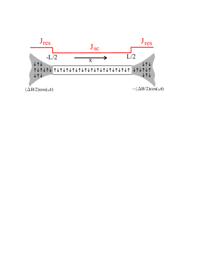
Figure 1: (color online) Schematic of a quantum spin chain coupled to magnetization reservoirs. The magnetic field bias $\Delta B$ changes periodically in time. In the upper part of the figure, we illustrate that the exchange coupling in the spin chain $J_{\rm sc}$ (for $|x|<L/2$) can in general be different from the exchange coupling in the grey-shaded magnetization reservoirs $J_{\rm res}$. As suggested in Ref. meier2003 , this setup can be realized by a bulk material with an intra-chain exchange much stronger than the inter-chain exchange, where the material is heated to a temperature $T>T_{N}$ in the central part and cooled to $T\ll T_{N}$ in the reservoir parts. ($T_{N}$ is the Néel ordering temperature.)

In order to describe the system shown in Fig. 1, we consider a one-dimensional XXZ spin chain in the presence of a time-dependent magnetic field $\mathbf{B}(\mathbf{x}_{i},t)=B_{i}(t)\mathbf{e}_{z}$ which can be described by the Hamiltonian $H=H_{\rm XXZ}+H_{B}(t)$, where

$$H_{\rm XXZ} = J\sum_{\langle i,j\rangle}\Bigl{(}s_{i,x}s_{j,x}+s_{i,y}s_{j,y}+\Delta s_{i,z}s_{j,z}\Bigr{)},$$ (1)

$$H_{B}(t) = g_{e}\mu_{B}\sum_{i}B_{i}(t)s_{i,z}.$$ (2)

Here, $s_{i,\alpha}$ is the $\alpha$-component of the spin operator at $\mathbf{x}_{i}$, $\langle i,j\rangle$ denotes nearest neighbor sites, $g_{e}$ is the g-factor, $\mu_{B}$ Bohr’s magneton, and we assume anti-ferromagnetic coupling with $J,\Delta>0$. A possible realization of spin chains described by $H_{\rm XXZ}$ is, for instance, a bulk structure of KCuF₃ or Sr₂CuO₃, where the exchange among different chains in the crystal is much weaker than the intra-chain exchange tennant1995 ; solog2001 ; hess2001 . It is well-known that the Hamiltonian $H_{\rm XXZ}$ can be mapped onto a LL of spinless fermions haldane1980 ; affleck1989 ; fradkin1991

$$H_{\rm LL}=\frac{\hbar v}{2}\int dx\left[g(\Pi(x))^{2}+\frac{1}{g}\left(\partial_{x}\varphi(x)\right)^{2}\right],$$ (3)

where we have ignored Umklapp scattering foot1 and made the identifications $v=v_{B}/g$, $v_{B}=Ja\sin(k_{B}a)/\hbar$, and $g=(1+4\Delta/\pi)^{-1/2}$ ($a$ is the lattice constant). In Eq. (3), $\varphi(x)$ is the standard Bose field operator in bosonization associated with spinon excitations here, $\Pi(x)$ its conjugate momentum density, $v$ the spinon velocity, $v_{B}$ the bare spinon velocity (at $\Delta=0$), $k_{B}$ the bare spinon wave vector, and $g$ the interaction parameter ($g=1$ corresponding to a non-interacting system, i.e. $\Delta=0$, and, in general for a $H_{\rm XXZ}$ spin chain, $1/2\leq g\leq 1$) gogolin1999 ; giamarchi2004 .

In order to be able to properly describe the effect of reservoirs, we modify the Hamiltonian $H_{\rm LL}$ in the spirit of the inhomogeneous LL model maslov1995 ; ponomarenko1995 ; safi1995 described by a Hamiltonian $H_{\rm ILL}$, where we assign a spatial dependence to $v$ and $g$ such that $v(x)=v_{l}$ and $g(x)=g_{l}$ being the spinon velocity and the interaction parameter in the reservoirs (for $|x|>L/2$), respectively, and $v(x)=v_{w}$ and $g(x)=g_{w}$ being the corresponding quantities in the spin chain region (for $|x|<L/2$). Within this model, non-equilibrium transport phenomena such as the non-linear $I-V$ characteristics and the current noise in the presence of impurities have been analyzed extensively peca2003 ; dolcini2003 ; trauzettel2004 ; dolcini2005 ; recher2006 . In this letter, we are interested in a different situation, namely the ac magnetization transport in the linear response regime which should be seen complementary to the electric ac response analyzed in Ref. cuni1998 ; safi1999a .

The Hamiltonian $H_{B}(t)$ describes a spatially varying and time-dependent magnetic field $\delta B(x)\cos(\omega t)\mathbf{e}_{z}$ with $\delta B(x)=-\Delta B/2$ ($\Delta B/2$) for $x<-L/2$ ($x>L/2$). For $|x|<L/2$, $\delta B(x)$ interpolates smoothly between the values $\pm\Delta B/2$ in the reservoirs foot2 . The dc ($\omega=0$) magnetization transport of such a system has been analyzed in Ref. meier2003 and a spin conductance $G_{s}=g_{l}(g_{e}\mu_{B})^{2}/h$ has been predicted.

The magnetization current in linear response to an oscillating magnetic field can be evaluated using the following expression

$$I_{m}(x,t)=\int_{-\infty}^{\infty}d\tau\int_{-\infty}^{\infty}dy\sigma_{0}(x,y,\tau)\partial_{y}\delta B(y,t-\tau)$$ (4)

with

$$\sigma_{0}(x,y,\tau)=2i\frac{(g_{e}\mu_{B})^{2}}{h}\Theta(\tau)\partial_{\tau}\Bigl{\langle}[\varphi(x,\tau),\varphi(y,0)]\Bigr{\rangle}$$ (5)

and the expectation value is taken with respect to $H_{\rm ILL}$. For $x>L/2$ and $|y|\leq L/2$, the spin conductivity is given by

$$\sigma_{0}(x,y,\tau)=g_{l}\frac{(g\mu_{B})^{2}}{h}(1-\gamma)\Theta(\tau)\sum_{p=0}^{\infty}\sum_{\alpha=\pm}\times$$ (6)

$$\Bigl{\{}\gamma^{2p}\delta\Bigl{(}\tau+\alpha\Bigl{(}\frac{x-L/2}{v_{l}}+\frac{L/2-y}{v_{w}}+\frac{2pL}{v_{w}}\Bigr{)}\Bigr{)}+$$

$$\gamma^{2p+1}\delta\Bigl{(}\tau+\alpha\Bigl{(}\frac{x-L/2}{v_{l}}+\frac{L/2+y}{v_{w}}+\frac{(2p+1)L}{v_{w}}\Bigr{)}\Bigr{)}\Bigr{\}},$$

where $\gamma=(g_{l}-g_{w})/(g_{l}+g_{w})$ is the reflection coefficient of spinon excitations at a sharp boundary with different interaction coefficients $g_{l}$ and $g_{w}$ safi1995 and $\Theta(\tau)$ the Heaviside function. The resulting spin current under continuous wave radiation reads

$$I^{({\rm cw})}_{m}(x,t)=2(1-\gamma)\frac{g_{l}v_{w}}{\omega}\frac{(g_{e}\mu_{B})^{2}}{h}\frac{\Delta B}{L}\sum_{p=0}^{\infty}\gamma^{2p}\times$$

$$\sin\Bigl{(}\frac{\omega L}{2v_{w}}\Bigr{)}\Bigl{\{}\cos\Bigl{[}\omega\left(t-\frac{(2p+1/2)L}{v_{w}}+\frac{L-2x}{2v_{l}}\right)\Bigr{]}$$

$$+\gamma\cos\Bigl{[}\omega\left(t-\frac{(2p+3/2)L}{v_{w}}+\frac{L-2x}{2v_{l}}\right)\Bigr{]}\Bigr{\}}.$$ (7)

We clearly observe an interaction-dependence of the magnetization current in Eq. (AC magnetization transport and power absorption in non-itinerant spin chains) through $g_{l}$ and $\gamma$. The presence of higher harmonics due to higher order terms in $\gamma^{m}$ would be a strong experimental evidence for the spatial inhomogeneity of spin-spin coupling in realizations of XXZ spin chains. The physics behind the result in Eq. (AC magnetization transport and power absorption in non-itinerant spin chains) is the following one: the system is driven with a continuous wave due to the ac magnetization source; therefore spinon excitations constantly enter and leave the spin chain from and to the reservoirs. Whenever, they experience a boundary in the exchange interaction, they are partly transmitted and partly reflected with a reflection coefficient $\gamma$. The resulting expression (AC magnetization transport and power absorption in non-itinerant spin chains) is the superposition of all possible contributions to the spin current after infinitely many reflection processes.

As a natural consequence, one may wonder whether an initial magnetization signal is actually transmitted through the spin chain. This depends crucially on the value of $\gamma$. To answer this question, we look at the magnetization current in linear response to a unit pulse described by $\partial_{y}\delta B(y,t)=\delta B_{p}\delta\tau_{p}\delta(t-t_{0})\delta(y-y_{0})$ with $y_{0}\in[-L/2,L/2]$ (where $\delta B_{p}$ corresponds to the height and $\delta\tau_{p}$ to the duration of the pulse). If we plug this expression into Eq. (4), we obtain for the spin current

$$I^{({\rm pul})}_{m}(x,t)=g_{l}\delta B_{p}\delta\tau_{p}\frac{(g_{e}\mu_{B})^{2}}{h}(1-\gamma)\Theta(t-t_{0})\sum_{p=0}^{\infty}\times$$

$$\sum_{\alpha=\pm}\Bigl{\{}\gamma^{2p}\delta\Bigl{(}\tau+\alpha\Bigl{[}\frac{x-L/2}{v_{l}}+\frac{L/2-y_{0}}{v_{w}}+\frac{2pL}{v_{w}}\Bigr{]}\Bigr{)}+$$

$$\gamma^{2p+1}\delta\Bigl{(}\tau+\alpha\Bigl{[}\frac{x-L/2}{v_{l}}+\frac{L/2+y_{0}}{v_{w}}+\frac{(2p+1)L}{v_{w}}\Bigr{]}\Bigr{)}\Bigr{\}}.$$

The derivation of $I^{({\rm pul})}_{m}(x,t)$ demonstrates that the initially sharp $\delta$-pulse is decomposed into a sum of infinitely many $\delta$-pulses. Importantly, the amplitude of these pulses decreases by a factor $\gamma$ in a stepwise fashion once in each time interval $L/v_{w}$ corresponding to the transit time in the wire. So, to answer the question how much signal has been transmitted we have to fix $x$, $y_{0}$, $t_{0}$, and $\gamma$ in Eq. (AC magnetization transport and power absorption in non-itinerant spin chains) and sum up all the prefactors of the $\delta$-functions that can be non-zero in a given time interval between $t_{0}$ and $t$. This analysis implies that all the dissipation happens in the leads and intrinsic relaxation is absent which is a direct consequence of the fact that the LL Hamiltonian describes a free boson. Once we introduce impurities the situation is different and intrinsic dissipation matters which we will briefly address below.

We now turn to the discussion of the power absorption under continuous wave radiation. It turns out that the absorbed power is an ideal physical quantity to measure the reflection coefficient $\gamma$. We derive the absorbed power of the 1D spin chain using Fermi’s golden rule and linear response theory where particular care has to be taken of the spatial inhomogeneity of systems. The resulting expression is

$$W(\omega)=\frac{1}{2}\left\{\int_{-L/2}^{L/2}dx\int_{-L/2}^{L/2}dy{\rm Re}\,\sigma_{0}(x,y,\omega)\right\}\left|\frac{\Delta B}{L}\right|^{2},$$ (9)

where

$${\rm Re}\,\sigma_{0}(x,y,\omega) = g_{w}\frac{(g_{e}\mu_{B})^{2}}{h}\Bigl{\{}\cos({\tilde{\omega}}({\tilde{x}}-{\tilde{y}}))$$

$$+ \frac{2\gamma(1-\gamma^{2})\cos({\tilde{\omega}})\cos({\tilde{\omega}}({\tilde{x}}+{\tilde{y}}))}{1+\gamma^{4}-2\gamma^{2}\cos(2{\tilde{\omega}})}$$

$$+ \frac{2\gamma^{2}\cos({\tilde{\omega}}({\tilde{x}}-{\tilde{y}}))(\cos(2{\tilde{\omega}})-\gamma^{2})}{1+\gamma^{4}-2\gamma^{2}\cos(2{\tilde{\omega}})}\Bigr{\}},$$

and we have introduced dimensionless variables ${\tilde{x}}=x/L$, ${\tilde{y}}=y/L$, and ${\tilde{\omega}}=\omega/\omega_{L}$ with $\omega_{L}=v_{w}/L$. It is straightforward to do the two remaining integrals in Eq. (9) and the final result reads

$$W(\omega) = g_{w}\frac{(g_{e}\mu_{B}\Delta B)^{2}}{2h}\left(\frac{\sin({\tilde{\omega}}/2)}{{\tilde{\omega}}/2}\right)^{2}$$

$$\times \frac{1-\gamma^{4}+2\gamma(1-\gamma^{2})\cos({\tilde{\omega}})}{1+\gamma^{4}-2\gamma^{2}\cos(2{\tilde{\omega}})}.$$

This is the main result of our work. It demonstrates that a measurement of the absorbed power due to ac response of the quantum spin chain is a simple and feasible way to measure interaction dependent coefficients such as $g_{w}$ and $\gamma$. In Eq. (AC magnetization transport and power absorption in non-itinerant spin chains), these coefficients just appear as pre-factors and not in a complicated power-law fashion as it is usually the case in observable quantities of systems described by LL physics. In Fig. 2, we show the interaction dependence of the absorbed power $W(\omega)$. This demonstrate that stronger repulsive interactions inside the wire with respect to the leads suppress the dissipative power.

If we compare Eqs. (AC magnetization transport and power absorption in non-itinerant spin chains) and (AC magnetization transport and power absorption in non-itinerant spin chains) we observe an interesting finite-size effect, namely that $W(\omega)$ vanishes as $(\sin({\tilde{\omega}}/2))^{2}$ close to $\tilde{\omega}\approx 2\pi$ whereas the leading contribution to $I_{m}^{({\rm cw})}(x,t)$ vanishes only as $\sin({\tilde{\omega}}/2)$ close to that driving frequency. Thus, the power absorption is more strongly suppressed than the magnetization current at frequencies close to $2\pi\omega_{L}$. This feature can be used in future devices to transfer data at special frequencies with low power dissipation.

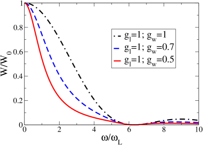
Figure 2: (color online) The absorbed power is shown in units of $W_{0}\equiv(g_{e}\mu_{B}\Delta B)^{2}/2h$ as a function of the ac frequency $\omega$ in units of the ballistic frequency $\omega_{L}=v_{w}/L$. It is clearly visible that stronger repulsive interactions inside the wire decrease the absorbed power in the system.

In the limit $\omega\rightarrow 0$, we obtain $W(0)=g_{l}(g_{e}\mu_{B}\Delta B)^{2}/2h$ corresponding to Joule heating where $W(0)=I_{m}^{2}(\omega=0)/(2G_{s})$.

We now address the robustness of our main result (AC magnetization transport and power absorption in non-itinerant spin chains) against impurity scattering. An impurity can be modeled as an altered link in the $H_{\rm XXZ}$ chain, i.e. a local change in $J$ on a nearest-neighbor link kane1992 ; eggert1992 . Within bosonization, such a scatterer at position $x_{0}$ in the system can be written as $H_{I}=\lambda\cos[\sqrt{4\pi}\varphi(x_{0},t)+2k_{B}x_{0}]$. If one of the two energy scales $\hbar v_{w}/L$ or $\hbar\omega$ is larger than $\lambda$ (the bare impurity strength), we can treat $H_{I}$ perturbatively up to lowest non-trivial order (which is second order in $\lambda$). In the presence of impurity scattering, the spin conductivity that enters into the calculation of Eq. (9) is subject to a (small) correction $\sigma_{I}(x,y,\omega)$ which has been derived for the corresponding electric case in Ref. dolcini2005 . For finite frequencies, $\sigma_{I}(x,y,\omega)$ needs to be evaluated numerically. In the zero frequency limit, one finds power-law corrections to the spin conductance maslov1995b ; safi1999b resulting in power-law corrections to the absorbed power. In any case, as long as either $\hbar v_{w}/L$ or $\hbar\omega$ are larger than the local change in $J$ of the sample, the effect of impurity scattering is weak.

The system which we considered previously consists of a spin chain smoothly connected to reservoirs. One may wonder how the previous result gets modified for isolated finite size spin chains, to which a time-dependent oscillating magnetic field is applied along the chain (such that $dB(x,t)/dx=\Delta B\cos(\omega t)$). For long Heisenberg chains, $H_{\rm XXZ}$ still maps onto a LL of spinless fermions as in Eq. (3) but with open boundary conditions (OBC). Following Ref. mattsson , we can establish that ${\rm Re}\,\sigma_{0}^{OBC}(x,y,\omega)=2g_{w}\frac{(g_{e}\mu_{B})^{2}}{h}\sin(\omega x/v_{w})\sin(\omega y/v_{w})$ for $\omega=\omega_{n}\equiv\pi nv_{w}/L$ ($n=1,\cdots,(L-a)/a$) and $0$ otherwise. From this expression, we can infer directly the power needed to spatially shake the spin chain, using Eq. (9),

$$W_{\rm OBC}(\omega)=g_{w}\frac{(g_{e}\mu_{B}\Delta B)^{2}}{h}\left(\frac{\sin({\tilde{\omega}}/2)}{{\tilde{\omega}}/2}\right)^{2}\sin^{2}({\tilde{\omega}}/2),$$ (12)

for $\tilde{\omega}=\omega_{n}/\omega_{L}$ and $0$ otherwise. Note that this power cannot be identified as dissipative power because a disconnected LL does not contain a dissipative term. Instead, $W_{\rm OBC}(\omega)$ is the work per unit time needed to shake the system. This is the major difference to the case with leads, i.e. Eq. (AC magnetization transport and power absorption in non-itinerant spin chains), where dissipation happens in the reservoirs. In the limit $\omega\to 0$, $W_{\rm OBC}\to 0$ due to the absence of reservoirs.

Let us now compare typical values for the absorbed power in electric systems versus magnetic systems. We set $g_{l}=g_{w}=1$ for simplicity but keep in mind how finite interactions change the power absorption according to Eq. (AC magnetization transport and power absorption in non-itinerant spin chains). The absorbed electric power in the dc limit is given by $W_{\rm el}=(e\Delta V)^{2}/h$. For a typical electric bias of $\Delta V=1$mV, we obtain $W_{\rm el}\approx 3.87\cdot 10^{-11}$Js^-1 whereas the absorbed magnetic power for a typical magnetic bias of $\Delta B=0.1$T is $W\approx 2.59\cdot 10^{-15}$Js^-1 (assuming $g_{e}=2$) which is four orders of magnitude smaller. The rule of the thumb is $W_{\rm el}(\Delta V=0.1{\rm mV})\sim W(\Delta B=1{\rm T})$. Thus, we expect substantial advantages of magnetic systems versus electric systems as far as power consumption is concerned.

In summary, we have analyzed the magnetization current and the power absorption of quantum spin chains coupled to magnetization reservoirs with a time-dependent magnetic field applied to the reservoirs. Both physical quantities depend crucially on the difference of the exchange interactions within the wire as compared to the magnetization leads. In fact, we envision to use this dependence as a way to control power dissipation in non-itinerant quantum systems in which magnetization transport occurs via spinons. Finally, we have briefly described the case of a finite size chain and the influence of impurity scattering on spin current.

We acknowledge financial support by the Swiss NSF, NCCR Nanoscience, and JST ICORP.

References

- (1) K.C. Hall and M.E. Flatté, Appl. Phys. Lett. 88, 162503 (2006).
- (2) I.V. Ovchinnikov and K.L. Wang, Appl. Phys. Lett. 92, 093503 (2008).
- (3) S.A. Wolf et al., Science 294, 1488 (2001).
- (4) Semiconductor Spintronics and Quantum Computation, edited by D.D. Awschalom, D. Loss, and N. Samarth (Springer-Verlag, Berlin, 2002).
- (5) D.D. Awschalom and M.E. Flatté, Nature Phys. 3, 153 (2007).
- (6) F. Meier and D. Loss, Phys. Rev. Lett. 90, 167204 (2003).
- (7) D.L. Maslov and M. Stone, Phys. Rev. B 52, R5539 (1995).
- (8) V.V. Ponomarenko, Phys. Rev. B 52, R8666 (1995).
- (9) I. Safi and H.J. Schulz, Phys. Rev. B 52, R17040 (1995).
- (10) D.A. Tennant et al., Phys. Rev. B 52, 13368 (1995).
- (11) A.V. Sologubenko et al., Phys. Rev. B 64, 054412 (2001).
- (12) C. Hess et al., Phys. Rev. B 64, 184305 (2001).
- (13) F.D.M. Haldane, Phys. Rev. Lett. 45, 1358 (1980).
- (14) I. Affleck, J. Phys. Condens. Matter 1, 3047 (1989).
- (15) E. Fradkin, Field Theories of Condensed Matter Systems (Addison-Wesley, Reading, 1991).
- (16) The Umklapp scattering term , where , that we have ignored in Eq. (3), is an irrelevant term (in a renormalization group sense) for which corresponds to .
- (17) A.O. Gogolin, A.A. Nersesyan, and A.M. Tsvelik, Bosonization and Strongly Correlated Systems (Cambridge University Press, Cambridge, 1999).
- (18) T. Giamarchi, Quantum Physics in One Dimension (Oxford University Press, Oxford, 2004).
- (19) C.S. Peca, L. Balents, and K.J. Wiese, Phys. Rev. B 68, 205423 (2003).
- (20) F. Dolcini et al., Phys. Rev. Lett. 91, 266402 (2003).
- (21) B. Trauzettel et al., Phys. Rev. Lett. 92, 226405 (2004).
- (22) F. Dolcini et al., Phys. Rev. B 71, 165309 (2005).
- (23) P. Recher, N.Y. Kim, and Y. Yamamoto, Phys. Rev. B 74, 235438 (2006).
- (24) G. Cuniberti, M. Sassetti, and B. Kramer, Phys. Rev. B 57, 1515 (1998).
- (25) I. Safi, Eur. Phys. J. B 12, 451 (1999).
- (26) We assume that is a long time-scale as compared to typical relaxation times in the reservoirs such that a local thermal equilibrium is established in both reservoirs. Furthermore, we request that , where is the high-energy cutoff frequency of the LL model. Additionally, we assume that the wire is isolated and the spinon number is conserved.
- (27) C.L. Kane and M.P.A. Fisher, Phys. Rev. B 46, 15233 (1992).
- (28) S. Eggert and I. Affleck, Phys. Rev. B 46, 10866 (1992).
- (29) D.L. Maslov, Phys. Rev. B 52, R14368 (1995).
- (30) I. Safi and H.J. Schulz, Phys. Rev. B 59, 3040 (1999).
- (31) A. E. Mattsson, S. Eggert, and H. Johannesson, Phys. Rev. B 56, 15615 (1997).