The Berry–Tabor conjecture for spin chains of Haldane–Shastry type

Abstract

According to a long-standing conjecture of Berry and Tabor, the distribution of the spacings between consecutive levels of a “generic” integrable model should follow Poisson’s law. In contrast, the spacings distribution of chaotic systems typically follows Wigner’s law. An important exception to the Berry–Tabor conjecture is the integrable spin chain with long-range interactions introduced by Haldane and Shastry in 1988, whose spacings distribution is neither Poissonian nor of Wigner’s type. In this letter we argue that the cumulative spacings distribution of this chain should follow the “square root of a logarithm” law recently proposed by us as a characteristic feature of all spin chains of Haldane–Shastry type. We also show in detail that the latter law is valid for the rational counterpart of the Haldane–Shastry chain introduced by Polychronakos.

I Introduction

It is well known Guhr et al. (1998) that the distribution of (suitably normalized) spacings between consecutive eigenvalues for the Gaussian ensembles in random matrix theory is approximately given by Wigner’s surmise

$$p(s)=(\pi/2)\mspace{1.0mu}s\exp(-\pi s^{2}/4)\,.$$

This behavior, which was first observed in the spectra of complex atomic nuclei, also seems to be characteristic of quantum chaotic systems like polygonal billiards Mehta (2004). On the other hand, for a “generic” quantum integrable system Berry and Tabor have conjectured Berry and Tabor (1977) that the spacings distribution should instead follow Poisson’s law $p(s)=\mathrm{e}^{-s}$. Over the years, this conjecture has been verified for many integrable models of physical interest, such as the Heisenberg chain, the $t$-$J$ model, the Hubbard model Poilblanc et al. (1993) and the chiral Potts model d’Auriac et al. (2002). In a recent paper Finkel and González-López (2005) it has been shown that there is an important exception to Berry and Tabor’s conjecture, namely the integrable spin chain introduced by Haldane and Shastry in 1988 Haldane (1988); Shastry (1988), whose spacings distribution follows neither Poisson’s nor Wigner’s law. It is the purpose of this letter to gain a deeper understanding of this fact, and to explore whether this property is shared by the analogous chain introduced by Polychronakos in ref. Polychronakos (1993).

The (antiferromagnetic) Haldane–Shastry (HS) spin chain describes a system of $N$ spins equally spaced on a circle with long-range exchange interactions inversely proportional to the square of the chord distance between the spins. More precisely, its Hamiltonian is given by

$${\mathcal{H}}_{\mathrm{HS}}=\frac{1}{2}\sum_{i<j}\sin(\vartheta_{i}-\vartheta_{j})^{-2}(1+S_{ij}),\qquad\vartheta_{k}=\frac{k\pi}{N}\,,$$ (1)

where $S_{ij}$ is the operator permuting the $i$-th and $j$-th spins. (Unless otherwise stated, throughout the paper all sums and products run from $1$ to $N$.) The HS chain is closely related to the Hubbard model; for instance, the chain’s ground state coincides exactly with Gutzwiller’s variational wave function for the Hubbard model when the on-site interaction tends to infinity Hubbard (1963); Gutzwiller (1963); Gebhard and Vollhardt (1987). Another important characteristic of the HS chain is its connection with the Sutherland spin model of $A_{N}$ type Sutherland (1971, 1972); Ha and Haldane (1992); Hikami and Wadati (1993); Minahan and Polychronakos (1993), from which it can be obtained by means of the so-called “freezing trick” Polychronakos (1993). This technique essentially consists in taking the strong coupling limit in the spin Sutherland model, so that the internal and dynamical degrees of freedom decouple and the spins become frozen at the equilibrium positions of the scalar part of the potential, which are precisely the chain sites $\vartheta_{k}$. This procedure can in fact be applied to all spin models of Calogero and Sutherland type, associated with both the $A_{N}$ and $BC_{N}$ roots systems in Olshanetsky and Perelomov’s scheme Olshanetsky and Perelomov (1983). For instance, the spin Calogero model of $A_{N}$ type Calogero (1971); Minahan and Polychronakos (1993)

$$H=-\sum_{i}\partial_{x_{i}}^{2}+a^{2}\sum_{i}x_{i}^{2}+a\sum_{i\neq j}\frac{a+S_{ij}}{(x_{i}-x_{j})^{2}}$$ (2)

yields the Hamiltonian of the so-called Polychronakos–Frahm (PF) spin chain Polychronakos (1993); Frahm (1993)

$${\mathcal{H}}_{\mathrm{PF}}=\sum_{i<j}(\xi_{i}-\xi_{j})^{-2}(1+S_{ij})\,.$$ (3)

The sites of this chain are the coordinates of the unique critical point of the scalar part of the potential of the Hamiltonian (2) in the domain $x_{1}<\cdots<x_{N}$, namely the numbers $\xi_{1}<\cdots<\xi_{N}$ determined by the algebraic system

$$\xi_{i}=2\sum_{j,j\neq i}\frac{1}{(\xi_{i}-\xi_{j})^{3}}\,,\qquad i=1,\dots,N\,.$$ (4)

Remarkably, these numbers are just the roots of the Hermite polynomial of degree $N$, as first pointed out by Calogero Calogero (1977).

In order to compute the spacings distributions of a spectrum, it is first necessary to transform the “raw” spectrum by applying the so-called unfolding mapping Haake (2001). This mapping is defined by decomposing the cumulative level density $F({\mathcal{E}})$ as the sum of a fluctuating part $F_{\mathrm{f{}l}}({\mathcal{E}})$ and a continuous part $\eta({\mathcal{E}})$, which is then used to transform each energy ${\mathcal{E}}_{i}$, $i=1,\dots,n$, into an unfolded energy $\eta_{i}=\eta({\mathcal{E}}_{i})$. In this way one obtains a uniformly distributed spectrum $\{\eta_{i}\}_{i=1}^{n}$, regardless of the initial level density. One finally considers the normalized spacings $s_{i}=(\eta_{i+1}-\eta_{i})/\Delta$, where $\Delta=(\eta_{n}-\eta_{1})/(n-1)$ is the mean spacing of the unfolded energies, so that $\{s_{i}\}_{i=1}^{n-1}$ has unit mean. The analysis of the spacings distribution has been carried out so far for the original ($A_{N}$-type) HS chain Finkel and González-López (2005), its supersymmetric version Basu-Mallick and Bondyopadhaya (2006) and, very recently Barba et al. (2008), for the PF chain of $BC_{N}$-type introduced by Yamamoto and Tsuchiya Yamamoto and Tsuchiya (1996). The corresponding spacings distributions were found to be qualitatively very similar, and differed essentially from both Wigner’s and Poisson’s distributions.

For the PF chain of $BC_{N}$ type, we showed in ref. Barba et al. (2008) that for large $N$ the cumulative spacings distribution $P(s)\equiv\int_{0}^{s}p(t)\mspace{1.0mu}\mathrm{d}t$ was approximately given by

$$P(s)\simeq 1-\frac{2}{\sqrt{\pi}\,s_{\mathrm{max}}}\,\sqrt{\log\Big{(}\frac{s_{\mathrm{max}}}{s}\Big{)}}\,,$$ (5)

where $s_{\mathrm{max}}$ is the maximum spacing. In fact, the above approximation holds for any spectrum ${\mathcal{E}}_{1}\equiv{\mathcal{E}}_{\mathrm{min}}<\cdots<{\mathcal{E}}_{n}\equiv{\mathcal{E}}_{\mathrm{max}}$ obeying the following conditions:

(i)  The energies are equispaced, i.e., ${\mathcal{E}}_{i+1}-{\mathcal{E}}_{i}=d$ for $i=1,\dots,n-1$.

(ii)  The level density (normalized to unity) is approximately given by the Gaussian law

$$g({\mathcal{E}})=\frac{1}{\sqrt{2\pi}\sigma}\,\mathrm{e}^{-\frac{({\mathcal{E}}-\mu)^{2}}{2\sigma^{2}}}\,,$$ (6)

where $\mu$ and $\sigma$ are respectively the mean and the standard deviation of the spectrum.

(iii)  ${\mathcal{E}}_{\mathrm{max}}-\mu\,,\,\mu-{\mathcal{E}}_{\mathrm{min}}\gg\sigma$.

(iv)  ${\mathcal{E}}_{\mathrm{min}}$ and ${\mathcal{E}}_{\mathrm{max}}$ are approximately symmetric with respect to $\mu$, namely $|{\mathcal{E}}_{\mathrm{min}}+{\mathcal{E}}_{\mathrm{max}}-2\mu|\ll{\mathcal{E}}_{\mathrm{max}}-{\mathcal{E}}_{\mathrm{min}}$.

As shown in ref. Barba et al. (2008), the above assumptions lead to the formula (5) with the following explicit expression for $s_{\mathrm{max}}$:

$$s_{\mathrm{max}}=\frac{(n-1)d}{\sqrt{2\pi}\sigma}\,.$$ (7)

It is relatively straightforward to check Barba et al. (2008) that conditions (i)–(iv) are indeed satisfied by the PF chain of $BC_{N}$ type (with $d=1$). In the rest of this letter we shall discuss the applicability of the approximation (5) to the original ($A_{N}$-type) PF and HS chains. We shall see that conditions (i)–(iv) are all satisfied by the PF chain, so that eq. (5) is guaranteed to work in this case. On the other hand, we shall explain why the latter formula is still an excellent approximation for the HS chain, even if not all of the above conditions hold for this chain.

II The Polychronakos–Frahm chain

The initial step in our analysis of the statistical properties of the spectrum of the PF chain is the explicit knowledge of the partition function, which makes it possible to compute the energy levels and their degeneracies for relatively large values of $N$. As first shown by Polychronakos Polychronakos (1994), the partition function can be evaluated in closed form by applying the freezing trick to the spin Calogero model (2). We shall present here an alternative expression for the partition function of the PF chain, which is more amenable to numerical computations than Polychronakos’s original formula.

The starting point in our derivation is the identity

$$H=H^{\mathrm{sc}}+2a{\mathcal{H}}_{\mathrm{PF}}\big{|}_{\xi_{k}\to x_{k}}\,,$$

where $H^{\mathrm{sc}}=H\big{|}_{S_{ij\to 1}}$ is the Hamiltonian of the scalar Calogero model. As explained in Barba et al. (2008), this identity implies that for large $a$ the energies of $H$ are approximately of the form

$$E_{ij}\simeq E^{\mathrm{sc}}_{i}+2a{\mathcal{E}}_{j}\,,$$

where $E^{\mathrm{sc}}_{i}$ and ${\mathcal{E}}_{j}$ are two arbitrary eigenvalues of $H^{\mathrm{sc}}$ and ${\mathcal{H}}_{\mathrm{PF}}$. Although this relation cannot be used directly to compute the chain energies ${\mathcal{E}}_{j}$, one can use it to express the partition function ${\mathcal{Z}}_{\mathrm{PF}}$ of the PF chain as

$${\mathcal{Z}}_{\mathrm{PF}}(T)=\lim_{a\to\infty}\frac{Z(2aT)}{Z^{\mathrm{sc}}(2aT)}$$ (8)

in terms of the partition functions $Z$ and $Z^{\mathrm{sc}}$ of $H$ and $H^{\mathrm{sc}}$, respectively. Both of these partition functions can be readily computed. Indeed, in the scalar case the energies are given by Calogero (1971)

$$E^{\mathrm{sc}}_{\mathbf{n}}=E_{0}+2a\sum_{i}n_{i},\quad E_{0}\equiv aN\big{(}a(N-1)+1\big{)},$$ (9)

with $\mathbf{n}=(n_{1},\dots,n_{N})$, where $n_{1}\geqslant\cdots\geqslant n_{N}$ are nonnegative integers. Setting $q=\mathrm{e}^{-1/(k_{\mathrm{B}}T)}$ and neglecting the ground state energy $E_{0}$ (which will also be subtracted from the energies of $H$), we obtain

$$Z^{\mathrm{sc}}(2aT)=\sum_{n_{1}\geqslant\cdots\geqslant n_{N}\geqslant 0}q^{\sum\limits_{i}n_{i}}\,.$$

Calling $p_{j}=n_{j}-n_{j+1}$, $j=1,\dots,N-1$, and $p_{N}=n_{N}$, so that $\sum\limits_{i}n_{i}=\sum\limits_{i}\sum\limits_{j\geqslant i}p_{j}=\sum\limits_{j}jp_{j}$, we finally have

$$Z^{\mathrm{sc}}(2aT)=\sum_{p_{1},\dots,p_{N}\geqslant 0}q^{\sum\limits_{j}jp_{j}}=\prod_{i}\big{(}1-q^{i}\big{)}^{-1}\,.$$ (10)

The energies of the spin Hamiltonian $H$ are still given by the RHS of (9), but now there is a degeneracy factor $d_{\mathbf{n}}$ due to the spin Basu-Mallick et al. (1999). More precisely, if $m$ is the number of internal degrees of freedom ($su(m)$ spin) and

$$\mathbf{n}=\big{(}\overbrace{\vphantom{1}\nu_{1},\dots,\nu_{1}}^{k_{1}},\dots,\overbrace{\vphantom{1}\nu_{r},\dots,\nu_{r}}^{k_{r}}\big{)},\qquad\nu_{1}>\cdots>\nu_{r}\geqslant 0,$$

then

$$d_{\mathbf{n}}=\prod_{i=1}^{r}\binom{m}{k_{i}}\equiv d(\mathbf{k})\,,\qquad\mathbf{k}=(k_{1},\dots,k_{r})\,.$$

Therefore

$$Z(2aT)=\sum_{\mathbf{k}\in{\mathcal{P}}_{N}}\sum_{\nu_{1}>\cdots>\nu_{r}\geqslant 0}d(\mathbf{k})\,q^{\,\sum\limits_{i=1}^{r}k_{i}\nu_{i}}\,,$$ (11)

where ${\mathcal{P}}_{N}$ denotes the set of ordered partitions of $N$. Calling again $p_{j}=\nu_{j}-\nu_{j+1}>0$, $j=1,\dots,r-1$, and $p_{r}=\nu_{r}\geqslant 0$, we have

$$\sum_{i=1}^{r}k_{i}\nu_{i}=\sum_{i=1}^{r}k_{i}\sum_{j=i}^{r}p_{j}=\sum_{j=1}^{r}K_{j}p_{j}\,,$$

where $K_{j}=\sum\limits_{i=1}^{j}k_{i}$. Substituting the previous equation into (11) and proceeding as before we easily obtain

$$Z(2aT)=\sum_{\mathbf{k}\in{\mathcal{P}}_{N}}q^{\sum\limits_{i=1}^{r-1}K_{i}}\prod_{i=1}^{r}\frac{\binom{m}{k_{i}}}{1-q^{K_{i}}}\,.$$ (12)

Since $1\leqslant K_{1}<\cdots<K_{r-1}<K_{r}=N$, we can define $N-r$ natural numbers $K^{\prime}_{i}$ by

$$\{K^{\prime}_{1},\dots,K^{\prime}_{N-r}\}=\{1,\dots,N-1\}-\{K_{1},\dots,K_{r-1}\}\,.$$

From eqs. (8), (10) and (12), it immediately follows that the partition function of the PF chain can be written as

$${\mathcal{Z}}_{\mathrm{PF}}(T)=\sum_{\mathbf{k}\in{\mathcal{P}}_{N}}\prod_{i=1}^{r}\binom{m}{k_{i}}\cdot q^{\sum\limits_{i=1}^{r-1}K_{i}}\cdot\prod_{i=1}^{N-r}\big{(}1-q^{K^{\prime}_{i}}\big{)}\,.$$ (13)

One can show that the latter expression is equivalent to Polychronakos’s by arguing as in ref. Basu-Mallick et al. (2007). Moreover, in the latter reference it is shown that eq. (13) implies that the energies of the PF chain are given by

$${\mathcal{E}}(\boldsymbol{\delta})=\sum_{i=1}^{N-1}\delta_{i}i\,,$$ (14)

where the motif $\boldsymbol{\delta}=(\delta_{1},\dots,\delta_{N-1})$ is a sequence of $0$’s and $1$’s with at most $m-1$ consecutive $0$’s. From the previous formula it follows that the spectrum of the PF chain is a set of consecutive integers, so that condition (i) in the previous section is satisfied with spacing $d=1$. Hence the number of distinct energies $n$ is simply the difference ${\mathcal{E}}_{\mathrm{max}}-{\mathcal{E}}_{\mathrm{min}}+1$, where the minimum and maximum energies can be computed with the help of eq. (14). Indeed, the maximum energy is obviously obtained from the motif $(1,\dots,1)$, so that

$${\mathcal{E}}_{\mathrm{max}}=\sum_{i=1}^{N-1}i=\frac{1}{2}\,N(N-1)\,.$$ (15)

On the other hand, the minimum energy corresponds to the motif

$$\boldsymbol{\delta}=\big{(}\dots,1,\overbrace{0,\dots,0}^{m-1},1,\overbrace{0,\dots,0}^{m-1}\big{)},$$ (16)

in which $\delta_{i}=1$ for $i=N-j\mspace{1.0mu}m$ with $j=1,\dots,k\equiv\lfloor N/m\rfloor$. Thus

$${\mathcal{E}}_{\mathrm{min}} =\sum_{j=1}^{k}(N-j\mspace{1.0mu}m)=kN-\frac{m}{2}\,k(k+1)$$

$$=\frac{N^{2}}{2m}-\frac{N}{2}+\frac{l(m-l)}{2m}\,,\qquad l\equiv N\operatorname{mod}m\,.$$ (17)

We shall next examine the validity of the second condition in the previous section for the PF chain. In fact, eq. (13) for the partition function turns out to be very efficient for computing the spectrum of this chain for large values of $N$ (up to $N=26$ for $m=2$ or $N=20$ for $m=3$, using Mathematica™ on a personal computer). In this way we have ascertained that the level density obeys the Gaussian law (6); cf. fig. 1 for the case $N=25$ and $m=2$.

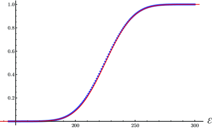
Figure 1: Cumulative energy density (at its discontinuity points) and its continuous approximation $\int_{-\infty}^{\mathcal{E}}g(t)\mathrm{d}t$ (continuous red line) for the PF chain with $N=25$ and $m=2$.

The mean energy $\mu$ and the variance $\sigma$ in eq. (6) can be computed in closed form for arbitrary values of $N$ and $m$ using several classical identities for the zeros of Hermite polynomials. More precisely, from the equality $\operatorname{tr}S_{ij}=m^{N-1}$ we easily obtain

$$\mu=\frac{\operatorname{tr}{\mathcal{H}}_{\mathrm{PF}}}{m^{N}} =\frac{1}{2}\,\Big{(}1+\frac{1}{m}\Big{)}\sum_{i\neq j}(\xi_{i}-\xi_{j})^{-2}$$

$$=\frac{1}{6}\,\Big{(}1+\frac{1}{m}\Big{)}\Big{[}2N(N-1)-\sum_{i}\xi_{i}^{2}\Big{]}\,,$$ (18)

where in the last equality we have used eq. (3.3b) of ref. Ahmed et al. (1979). In order to evaluate the last sum, we use the well-known identity (Ahmed et al., 1979, eq. (3.3a))

$$\sum_{j,j\neq i}\frac{1}{\xi_{i}-\xi_{j}}=\xi_{i}\,.$$ (19)

Since, by antisymmetry,

$$\sum_{i\neq j}\frac{\xi_{i}}{\xi_{i}-\xi_{j}}=\frac{1}{2}\,N(N-1)\,,$$

multiplying eq. (19) by $\xi_{i}$ and summing over $i$ we obtain

$$\sum_{i}\xi_{i}^{2}=\frac{1}{2}\,N(N-1)\,,$$ (20)

and therefore

$$\mu=\frac{1}{4}\,\Big{(}1+\frac{1}{m}\Big{)}N(N-1)\,.$$ (21)

Similarly, using the identity

$$\operatorname{tr}(S_{ij}S_{kl})=m^{N-2+2\delta_{ik}\delta_{jl}+2\delta_{il}\delta_{jk}}\,,$$

and proceeding as in ref. Enciso et al. (2005), we obtain

$$\sigma^{2}=\frac{\operatorname{tr}({\mathcal{H}}_{\mathrm{PF}}^{2})}{m^{N}}-\frac{(\operatorname{tr}{\mathcal{H}}_{\mathrm{PF}})^{2}}{m^{2N}}\\ =\frac{1}{2}\Big{(}1-\frac{1}{m^{2}}\Big{)}\sum_{i\neq j}(\xi_{i}-\xi_{j})^{-4}.$$ (22)

From (Ahmed et al., 1979, eq. (3.3d)) and (20) it follows that

$$45\sum_{i\neq j}(\xi_{i}-\xi_{j})^{-4}=N(N-1)(2N+7)+\sum_{i}\xi_{i}^{4}\,.$$ (23)

Multiplying eq. (19) by $\xi_{i}^{3}$ and summing over $i$ we obtain

$$\sum_{i}\xi_{i}^{4} =\sum_{i\neq j}\frac{\xi_{i}^{3}}{\xi_{i}-\xi_{j}}=\frac{1}{2}\sum_{i\neq j}\big{(}\xi_{i}^{2}+\xi_{i}\xi_{j}+\xi_{j}^{2}\big{)}$$

$$=\Big{(}N-\frac{3}{2}\Big{)}\sum_{i}\xi_{i}^{2}+\frac{1}{2}\Big{(}\sum_{i}\xi_{i}\Big{)}^{2}$$

$$=\frac{1}{2}\,N(N-1)\Big{(}N-\frac{3}{2}\Big{)}\,,$$ (24)

where we have used eq. (20) and the obvious identity $\sum_{i}\xi_{i}=0$. From eqs. (22), (23) and (24) we finally have

$$\sigma^{2}=\frac{1}{36}\Big{(}1-\frac{1}{m^{2}}\Big{)}N(N-1)\Big{(}N+\frac{5}{2}\Big{)}.$$ (25)

Equations (15), (II), (21) and (25) imply that both $({\mathcal{E}}_{\mathrm{max}}-\mu)/\sigma$ and $(\mu-{\mathcal{E}}_{\mathrm{min}})/\sigma$ grow as $N^{1/2}$ when $N\to\infty$, so that condition (iii) in the previous section is satisfied. The last of these conditions is also satisfied for large $N$, since by the equations just quoted $|{\mathcal{E}}_{\mathrm{min}}+{\mathcal{E}}_{\mathrm{max}}-2\mu|=O(N)$ while ${\mathcal{E}}_{\mathrm{max}}-{\mathcal{E}}_{\mathrm{min}}=O(N^{2})$. By the discussion in the previous section, it follows that the cumulative spacings distribution of the PF chain is approximately given by eq. (5) for large $N$. We have indeed verified that (5) holds with great accuracy by computing $P(s)$ for a wide range of values of $N$ and $m$ using eq. (13) for the partition function. For instance, in the case $N=25$ and $m=2$ presented in fig. 2 the RHS of (5) fits the numerical data with a mean square error of $8.4\times 10^{-5}$.

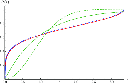
Figure 2: Cumulative spacings distribution $P(s)$ and its analytic approximation (5) (continuous red line) for the PF chain with $N=25$ and $m=2$. For convenience, we have also plotted Poisson’s (green, long dashes) and Wigner’s (green, short dashes) cumulative distributions.

It should be noted that the parameter $s_{\mathrm{max}}$ in the formula (5) for $P(s)$ can be computed explicitly as a function of $N$ and $m$ using (7) (with $d=1$), (25), the identity $n-1={\mathcal{E}}_{\mathrm{max}}-{\mathcal{E}}_{\mathrm{min}}$, and eqs. (15) and (II). In particular, for large $N$ the maximum spacing $s_{\mathrm{max}}$ behaves as

$$s_{\mathrm{max}}=\frac{3}{\sqrt{2\pi}}\,\sqrt{\frac{m-1}{m+1}}\>N^{1/2}+O\big{(}N^{-1/2}\big{)}\,,$$

just as for the PF chain of $BC_{N}$ type Barba et al. (2008). We thus conclude that for $N\gg 1$ the spacings distributions of the PF chains of $A_{N}$ and $BC_{N}$ types are asymptotically equal, in spite of the fact that the spectra of these models are quite different.

III The Haldane–Shastry chain

It is well-known that the spectrum of the original HS chain (1) is not equispaced, so that the first condition in section 1 does not hold in this case. However, it was recently noted Barba et al. (2008) that the cumulative spacings distribution of this chain can be still approximated with great accuracy by a function of the form (5). The parameter $s_{\mathrm{max}}$ is given again by eq. (7), but now $d$ is the spacing ${\mathcal{E}}_{i+1}-{\mathcal{E}}_{i}$ with highest frequency and $n$ is the total number of energy levels. As an example, in fig. 3 we present the plot of $P(s)$ and its approximation (5) in the case $N=25$ and $m=2$, for which $d=2$, $n=562$, and hence $s_{\mathrm{max}}\simeq 3.113$.

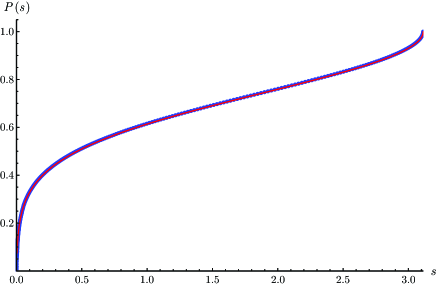
Figure 3: Cumulative spacings distribution $P(s)$ and its analytic approximation (5) (continuous red line) for the HS chain with $N=25$ and $m=2$. The mean square error of the fit is $1.8\times 10^{-5}$.

In the rest of this section we shall analyze why eq. (5) provides an excellent approximation to the cumulative spacings distribution of the HS chain, in spite of the fact that condition (i) in section 1 is not satisfied. We shall start by verifying that the remaining conditions (ii)–(iv) are satisfied in this case. In the first place, the fact that the level density is approximately Gaussian was established in ref. Finkel and González-López (2005), where it was also shown that the mean energy and its standard deviation are respectively given by

$$\mu =\frac{1}{12}\,\Big{(}1+\frac{1}{m}\Big{)}N(N^{2}-1)\,,$$ (26)

$$\sigma^{2} =\frac{1}{360}\Big{(}1-\frac{1}{m^{2}}\Big{)}\,N(N^{2}-1)(N^{2}+11)\,.$$ (27)

As to the third condition, recall that the maximum energy is given by Finkel and González-López (2005)

$${\mathcal{E}}_{\mathrm{max}}=\frac{N}{6}(N^{2}-1)\,.$$ (28)

The minimum energy can be computed from the analogue of eq. (14), which for the HS chain reads Haldane et al. (1992); Finkel and González-López (2005)

$${\mathcal{E}}(\boldsymbol{\delta})=\sum_{i=1}^{N-1}\delta_{i}i(N-i)\,,$$

where again $\boldsymbol{\delta}$ is a motif with at most $m-1$ consecutive $0$’s. It can be shown that the motif yielding the minimum energy is again given by (16) (or, alternatively, by the complementary motif $\boldsymbol{\delta}^{\prime}$ with $\delta^{\prime}_{i}=\delta_{N-i}$), so that

$${\mathcal{E}}_{\mathrm{min}}=\sum_{j=1}^{k}jm(N-jm)\,,$$

with $k=\lfloor N/m\rfloor$. Evaluating the latter sum we easily obtain

$${\mathcal{E}}_{\mathrm{min}}=\frac{1}{6m}\,(N-l)(N+m-l)(N-m+2l)\,,$$ (29)

where $l\equiv N\operatorname{mod}m$. Equations (26)–(29) imply that (as for the PF chain) $({\mathcal{E}}_{\mathrm{max}}-\mu)/\sigma$ and $(\mu-{\mathcal{E}}_{\mathrm{min}})/\sigma$ grow as $N^{1/2}$ when $N\to\infty$, so that condition (iii) is clearly satisfied. Finally, from the previous equations it follows that $|{\mathcal{E}}_{\mathrm{min}}+{\mathcal{E}}_{\mathrm{max}}-2\mu|=O(N)$ while ${\mathcal{E}}_{\mathrm{max}}-{\mathcal{E}}_{\mathrm{min}}=O(N^{3})$, which implies condition (iv).

We shall next discuss in more detail to what extent the first condition fails. To this end, we have used the formula for the partition function of the HS chain given in (Finkel and González-López, 2005, eq. (22)) to compute the spectrum for a wide range of values of $m$ and $N$ such that $m^{N}\leqslant 2^{28}$. Our results evidence that when $N$ is sufficiently large the vast majority of the differences $d_{i}\equiv{\mathcal{E}}_{i+1}-{\mathcal{E}}_{i}$ are equal to $d=1$ (for even $N$) or $d=2$ (for odd $N$), as shown in fig. 4. Thus, we can say that the spectrum of the HS chain is quasi-equispaced for large $N$. Moreover, our computations indicate that the differences $d_{i}\neq d$ correspond to energies ${\mathcal{E}}_{i}$ in the tail of the Gaussian distribution $g({\mathcal{E}})$; see, e.g., fig. 5 for the case $m=2$, $N=26$.

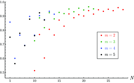
Figure 4: Ratio $\displaystyle\frac{\#(d_{i}=d)}{n-1}$ for the HS chain with $m=2,3,4,5$ and $N$ up to $28$.

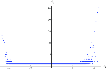
Figure 5: Differences $d_{i}\equiv{\mathcal{E}}_{i+1}-{\mathcal{E}}_{i}$ versus $\varepsilon_{i}\equiv({\mathcal{E}}_{i}-\mu)/\sigma$ for the HS chain with $N=26$ and $m=2$.

The two features of the spectrum of the HS chain just described provide the key to understanding why the formula (5), with $s_{\mathrm{max}}$ given by (7), still works remarkably well in this case. Indeed, since the level density is approximately Gaussian, we have

$$\eta({\mathcal{E}})=\int_{-\infty}^{\mathcal{E}}g(t)\mspace{1.0mu}\mathrm{d}t\,,$$

so that

$$\eta_{i+1}-\eta_{i}\equiv\eta({\mathcal{E}}_{i+1})-\eta({\mathcal{E}}_{i})\simeq\eta^{\prime}({\mathcal{E}}_{i})d_{i}=g({\mathcal{E}}_{i})d_{i}\,.$$

By condition (iii) in section 1 we have $\eta_{n}\simeq 1$ and $\eta_{1}\simeq 0$, and thus $\Delta\simeq 1/(n-1)$. Hence, the normalized spacings $s_{i}$ are approximately given by

$$s_{i}=\frac{\eta_{i+1}-\eta_{i}}{\Delta}\simeq(n-1)d_{i}\mspace{1.0mu}g({\mathcal{E}}_{i})\equiv\frac{(n-1)d_{i}}{\sqrt{2\pi}\sigma}\,\mathrm{e}^{-\frac{({\mathcal{E}}_{i}-\mu)^{2}}{2\sigma^{2}}}\,.$$

Since the few values of $d_{i}$ different from $d$ correspond to energies ${\mathcal{E}}_{i}$ several standard deviations away from $\mu$, their associated spacings $s_{i}$ turn out to be very small. Therefore, we can write with great accuracy

$$s_{i}\simeq\frac{(n-1)d}{\sqrt{2\pi}\sigma}\,\mathrm{e}^{-\frac{({\mathcal{E}}_{i}-\mu)^{2}}{2\sigma^{2}}}\equiv s_{\mathrm{max}}\,\mathrm{e}^{-\frac{({\mathcal{E}}_{i}-\mu)^{2}}{2\sigma^{2}}}\,,$$ (30)

except for a few spacings $s_{i}$ very small compared to $s_{\mathrm{max}}$; see, e.g., fig. 6 for the case $N=26$, $m=2$. As shown in ref. Barba et al. (2008), eq. (30) leads directly to the approximate formula (5) for the cumulative spacings distribution $P(s)$. This explains why the latter formula is also valid for the HS chain, with the value of $s_{\mathrm{max}}$ given in eq. (7).

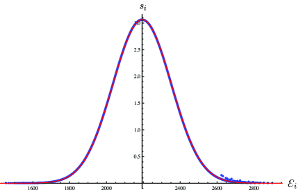
Figure 6: Comparison of the normalized spacings $s_{i}$ (blue dots) with the Gaussian distribution (30) (continuous red curve) for the HS chain with $N=26$ and $m=2$.