Landau levels on the 2-D torus: a numerical approach

Enrico Onofri ^a,b

Abstract

A numerical method is presented which allows to compute the spectrum of the Schroedinger operator for a particle constrained on a two dimensional flat torus under the combined action of a transverse magnetic field and any conservative force. The method employs a fast Fourier transform to accurately represent the momentum variables and takes into account the twisted boundary conditions required by the presence of the magnetic field. An accuracy of twelve digits is attained even with coarse grids. Landau levels are reproduced in the case of a uniform field satisfying Dirac’s condition. A new fine structure of levels within the single Landau level is formed when the field has a sinusoidal component with period commensurable to the integer magnetic charge.

PACS numbers: 31.15.-p, 71.70.Di

^a) Laboratoire de Physique Théorique et Astroparticules, Université Montpellier II, Place E. Bataillon, 34095 Montpellier Cedex 05, France.

^b) Permanent address: Università di Parma and INFN, Gruppo Collegato di Parma, 43100 Parma, Italy.

1. Introduction

The quantum mechanics of a charged particle living on a two-dimensional torus in presence of a uniform magnetic field, orthogonal to the surface, has been solved years ago [1, 2, 3]. The degeneration of the ground state coincides with the flux of the magnetic field, in units of the elementary flux $hc/e$ (in this paper we shall adopt units such that $\hslash=e/c=1$). This is a simple example of the more general theorem about cohomology groups for hermitian line bundles [4], known in the physical literature as Dirac’s quantization condition: quantum mechanics requires that the flux of the magnetic field across a closed surface must be quantized. This is also known as the Weil-Souriau-Kostant quantization condition.

In this paper we present a numerical algorithm which is accurate enough in representing the momentum variables and it respects the constraints posed by differential geometry. The algorithm computes the spectrum of the quantum particle on the torus in presence of both a transverse magnetic field and a scalar potential. If the potential vanishes and the magnetic field is uniform the algorithm reproduces the known spectrum, in terms of eigenvalues and degeneration, to a typical accuracy of twelve digits. The effect of the potential energy is to split the Landau Levels; this fact is at the basis of Klauder’s formulation of path integrals in phase space [5] and our algorithm could be used to explore this approach to quantization theory. The case of a non-uniform magnetic field and the corresponding splitting pattern of Landau levels can be studied using our algorithm. We consider the case of a sinusoidal contribution to the magnetic field in the last section. A peculiar fine structure emerges, which is made visible by the accuracy of the algorithm. This fine-structure within each Landau level could be dubbed Landau-Mathieu levels and it manifests itself when the number of oscillations of the perturbed field is commensurate to the quantized magnetic flux. This fact suggests that an undulating stationary magnetic field could be used to tune the number of states in the fine structure of Landau-Mathieu sub levels.

2. The model

Quantum mechanics on a compact surface, in the presence of a magnetic field transverse to the surface, requires the introduction of either a singular magnetic potential (Dirac’s string) or a collection of local potentials $A_{\alpha}$, one for each local chart of a given atlas on the surface. The description in terms of local potentials is preferable for its mathematical rigor [6]. The implementation of the local description within a numerical approach should be easily achieved in terms of finite elements methods. In this paper we take an alternative route, working on a single chart, but imposing the correct (twisted) boundary conditions to the wave function, as we explain in the next section.

3. Local charts and twisted boundary conditions

Let the torus be identified with the two-dimensional plane $\mathbb{R}^{2}$ modulo the discrete subgroup of translations generated by $x\to x+L_{1},y\to y+L_{2}$. We cover the torus with four charts defined as follows

(1) $$\begin{matrix}\mathcal{C}_{\alpha}:\begin{cases}0<x<L_{1}\phantom{+\delta_{2}}\\ 0<y<L_{2}\end{cases}&\mathcal{C}_{\beta}:\begin{cases}\delta_{1}<x<L_{1}+\delta_{1}\\ 0<y<L_{2}\end{cases}\\[1.99997pt] \mathcal{C}_{\gamma}:\begin{cases}0<x<L_{1}\\ \delta_{2}<y<L_{2}+\delta_{2}\end{cases}&\mathcal{C}_{\delta}:\begin{cases}\delta_{1}<x<L_{1}+\delta_{1}\\ \delta_{2}<y<L_{2}+\delta_{2}\end{cases}\end{matrix}$$

In each chart we define a local magnetic potential by

(2) $$\forall i:\boldsymbol{\mathcal{A}}_{i}=(-\mbox{\small$\frac{1}{2}$}By,\mbox{\small$\frac{1}{2}$}Bx)$$

(remember we use units where $e/c=1$). All local potentials are defined in the same way, but their values are different. Within the overlaps of the local charts we easily find the transition functions realizing the gauge transformations from one description to another. For instance, the chart $\beta$ overlaps $\alpha$ in two distinct regions, $\mathcal{I}^{(1)}_{\alpha\beta}=\{\delta_{1}<x_{\alpha}=x_{\beta}<L_{1}\}$ and $\mathcal{I}^{(2)}_{\alpha\beta}=\{0<x_{\alpha}<\delta_{1},L_{1}<x_{\beta}<L_{1}+\delta_{1}\}$. In the overlap $\mathcal{I}^{(1)}_{\alpha\beta}$ the value of the potentials coincide, while in $\mathcal{I}^{(2)}_{\alpha\beta}$ we have

(3) $$\begin{split}\boldsymbol{\mathcal{A}}_{\beta}&=\boldsymbol{\mathcal{A}}_{\alpha}+(0,\mbox{\small$\frac{1}{2}$}BL_{1})\\ &=\boldsymbol{\mathcal{A}}_{\alpha}+\nabla\chi_{\alpha\beta}\end{split}$$

with $\chi_{\alpha\beta}=\mbox{\small$\frac{1}{2}$}BL_{1}y$. The other transition functions are determined similarly. For instance in $\mathcal{I}^{(2)}_{\alpha\gamma}=\{0<y_{\alpha}<\delta_{2},L_{2}<y_{\gamma}<L_{2}+\delta_{2}\}$ it holds

(4) $$\begin{split}\boldsymbol{\mathcal{A}}_{\gamma}&=\boldsymbol{\mathcal{A}}_{\alpha}+(-\mbox{\small$\frac{1}{2}$}BL_{2},0)\\ &=\boldsymbol{\mathcal{A}}_{\alpha}+\nabla\chi_{\alpha\gamma}\end{split}$$

with $\chi_{\alpha\gamma}=-\mbox{\small$\frac{1}{2}$}BL_{2}x$.

Now, to build the Hamiltonian operator, which is formally given by the usual minimal coupling, one has to establish the transition functions proper to the local wave functions. As it is well-known these are obtained by exponentiating the transition functions, i.e.

(5) $$\psi_{\beta}(x,y)=e^{i\chi^{(j)}_{\alpha\beta}}\psi_{\alpha}(x,y)\qquad{\rm on}\;\mathcal{I}^{(j)}_{\alpha\beta}$$

Now take a sequence of points $s_{1}$ converging to $(L_{1},y)$ from the left and a second sequence $s_{2}$ converging from the right to the same point. On $s_{1}$ we have $\psi_{\alpha}=\psi_{\beta}\to\psi_{\alpha}(L_{1},y)$; on $s_{2}$ we have $\psi_{\beta}\to\psi_{\alpha}(0,y)\exp\{\mbox{\small$\frac{1}{2}$}i\,BL_{1}\,y\}$. By continuity of $\psi_{\beta}$ we get a condition on $\psi_{\alpha}$ namely

(6) $$\psi_{\alpha}(L_{1},y)=e^{\mbox{ $\scriptstyle\frac{1}{2}$}i\,BL_{1}\,y}\,\psi_{\alpha}(0,y)\,.$$

By a similar argument we find a second condition

(7) $$\psi_{\alpha}(x,L_{2})=e^{-\mbox{ $\scriptstyle\frac{1}{2}$}i\,BL_{2}\,x}\,\psi_{\alpha}(x,0)\,.$$

At this point we are allowed to work on a single local chart (let’s choose $\mathcal{C}_{\alpha}$) and the Hamiltonian is defined by

(8) $$H=\mbox{\small$\frac{1}{2}$}(-i\partial_{x}+\mbox{\small$\frac{1}{2}$}B\,y)^{2}\,+\mbox{\small$\frac{1}{2}$}(-i\partial_{y}-\mbox{\small$\frac{1}{2}$}B\,x)^{2}+V(x,y)$$

on a domain of differentiable functions satisfying Eq.s(6,7) as boundary conditions. Notice that the b.c. are only consistent if Dirac’s condition is satisfied. To see this, compute $\psi(L_{1},L_{2})$ by applying the b.c. in two different orders:

(9) $$\psi(L_{1},L_{2}) = \psi(0,L_{2})\,e^{\mbox{ $\scriptstyle\frac{1}{2}$}iBL_{1}L_{2}}=\psi(0,0)\,e^{\mbox{ $\scriptstyle\frac{1}{2}$}iBL_{1}L_{2}}$$

(10) $$\psi(L_{1},L_{2}) = \psi(L_{1},0)\,e^{-\mbox{ $\scriptstyle\frac{1}{2}$}iBL_{1}L_{2}}=\psi(0,0)\,e^{-\mbox{ $\scriptstyle\frac{1}{2}$}iBL_{1}L_{2}}$$

hence $\exp\{i\,B\,L_{1}\,L_{2}\}=1$. All this is well–known, but it was recalled here to introduce the main idea behind the algorithm we describe in the next section.

4. The algorithm

A simple code, based on a discrete approximation of partial derivatives, is easily produced; the twisted boundary conditions Eq.s (6, 7) are implemented without difficulty. However this methods has serious limitations in attaining good accuracies. A test run with $B=2\pi$, $L_{1}=L_{2}=2$ performed with a $64\times 64$ grid in configuration space yields the low energy spectrum (first 20 eigenvalues) with an average error of $1.5\%$. In particular the first four eigenvalues, which should coincide with $\pi$, turn out to be $\pi\times(0.9997,1.0082,1.0082,1.0419)$. With a finer mesh ($128\times 128$) the error improves ($0.5\%$) but the computing time grows considerably (from 25 sec to $\approx 400$ sec). This fact encourages to design an algorithm with a better accuracy on partial derivatives. This is achieved by using a “spectral method” based on the Fourier transform.

4.1. The spectral method

A very accurate representation of partial derivatives can be obtained by using Fourier transform, in one of its efficient implementations as a numerical code; we shall use FFTW [8], which is now included in Matlab. However, Fourier transform assumes a periodic wave-function, which is not the case with our problem. The way out is to apply FFT separately along $x$ and $y$; the $x$ transform is applied to the function $\phi=\exp\{-\mbox{\small$\frac{1}{2}$}iB\,x\,y\}\,\psi$, which turns out to be periodic in $x$ with period $L_{1}$. The minimal coupling is then recovered by realizing that

(11) $$(-i\partial_{x}+\mbox{\small$\frac{1}{2}$}B\,y)\,\psi\equiv e^{\mbox{\small$\frac{1}{2}$}iBxy}(-i\partial_{x}\phi)+B\,y\,\psi\;.$$

Now the partial derivative can be computed in $x-$Fourier space. Similarly $\phi=\exp\{\mbox{\small$\frac{1}{2}$}iB\,x\,y\}\,\psi$ is periodic in $y$ with the right period, and we may compute

(12) $$(-i\partial_{y}-\mbox{\small$\frac{1}{2}$}B\,x)\,\psi\equiv e^{-\mbox{\small$\frac{1}{2}$}iBxy}(-i\partial_{y}\phi)-B\,x\,\psi\;.$$

The idea is used to compute with high accuracy the action of the Hamiltonian on any function satisfying the twisted b.c.; this is then used as the unique piece of information needed by the Arnoldi algorithm to get the spectrum. We also have to choose an initial vector, if do not feel easy about a random initial vector. A function satisfying the boundary conditions can be constructed as follows. Choose any $\psi_{0}(x,y)$, e.g. a Gaussian centered in the middle of the rectangle of sides $L_{1},L_{2}$. Let $BL_{1}L_{2}=2\pi N$; then the following equation defines a “good” wave-function:

(13) $$\psi(x,y)=\sum_{n_{1},n_{2}}(-1)^{n_{1}\,n_{2}\,N}\,e^{\mbox{\small$\frac{1}{2}$}iBL_{2}\,x-\mbox{\small$\frac{1}{2}$}iBL_{1}\,y}\,\psi_{0}(x+n_{1}L_{1},y+n_{2}L_{2})$$

The series can be truncated if $\psi_{0}$ is a Gaussian with a width small with respect to $L_{i}$.

These are the ingredients which can be used to make a call to Matlab’s routine eigs, which provides a very friendly interface to the Arnoldi package Arpack[9]. The result is rather spectacular as we report next.

4.2. Test runs and error estimates

We apply the algorithm to a grid $n\times n$, starting with very coarse grids. In Tab.1 we report the average error and the timings to compute the first 20 eigenvalues with the same data as before.

n	Relative Error	Time (sec)
8	$1.8\times 10^{-2}$	0.15
10	$2.5\times 10^{-3}$	0.25
12	$5.3\times 10^{-7}$	0.35
16	$1.0\times 10^{-13}$	0.60
24	$1.8\times 10^{-13}$	1.35
32	$2.4\times 10^{-13}$	2.85
64	$6.0\times 10^{-13}$	24.7

Table 1.

As we see, the algorithm reproduces the correct spectrum (including degeneracy) already at very low $n$. The relative error saturates around $10^{-12}$ which seems to be inherent to the Arnoldi algorithm as implemented in Matlab (routine eigs).

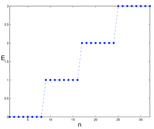
Figure 1. The Landau levels with $N=\tfrac{1}{2\pi}BL_{1}L_{2}=8$, in units of the Larmor frequency.

In Fig.1 we see a typical spectrum obtained with the algorithm. The degeneracy of the eigenvalues is within $10^{-12}$, obtained with a $32\times 32$ grid.

Let us notice that if we plug a value of $B$ which does not respect Dirac’c condition, the degeneracy is broken; this fact can be interpreted as due to the fact that there is a spurious singular contribution to the magnetic field at the boundary of the local chart which breaks the original symmetry.

Another check for accuracy can be performed by adding a potential energy $\mbox{\small$\frac{1}{2}$}\omega^{2}(x^{2}+y^{2})$, in which case the spectrum is known in the limit of large $L_{1}$ and $L_{2}$. In the case $B=2,\omega=1$, we get the spectrum $E=(n_{1}+\mbox{\small$\frac{1}{2}$})\omega_{1}+(n_{2}+\mbox{\small$\frac{1}{2}$})\omega_{2}$ with a relative error of $10^{-13}$ on a $64\times 64$ grid. The presence of a potential energy requires a relatively finer mesh.

5. Fine structure Landau-Mathieu levels

Having an algorithm which allows for accurate eigenvalue computations is like having a microscope with higher resolution power: you can resolve details which would otherwise be invisible. It came then as a surprise, using the new algorithm, to discover a structure in Landau levels when the uniform magnetic field is perturbed by an undulating additive contribution $B\to B(1+\lambda\sin(2\pi\nu x/L_{1})$. Notice that boundary conditions adapted to this choice of gauge fields must be reformulated, along the lines of Sec. 3. Fig.2 shows the splitting of the first Landau level which occurs at $\nu=4$.

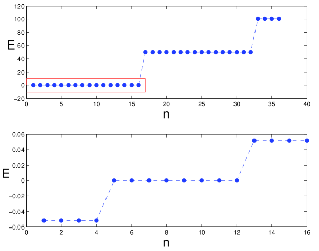
Figure 2. The fine structure pattern of the first Landau level, $\nu=4,N_{0}=16$. The picture below is a blow–up of the portion of the rectangle in the picture above.

The pattern is reproduced for other choices of parameters and it looks numerically very stable and degeneracy within the fine structure levels is observed numerically at 12 digits precision.(see Fig. 3). There are $N_{0}=\frac{1}{2\pi}BL_{1}L_{2}$ states in the first level; these are subdivided in finer sub-levels if $N_{0}$ is a multiple of $\nu$: degeneracy is given by the greatest common divisor ${\rm gcd}(N_{0},2\nu)$, hence it is destroyed if $N_{0}$ and $\nu$ are relatively prime, but it is left unchanged if $\nu$ is a multiple of $N_{0}$.

We also explored the stability of this phenomenon with respect to deformation of the magnetic field, by keeping its periodicity on the torus, e.g. by adding a higher harmonic contribution; the pattern of degeneracy stays the same, only the eigenvalues are shifted (see Fig. 4).

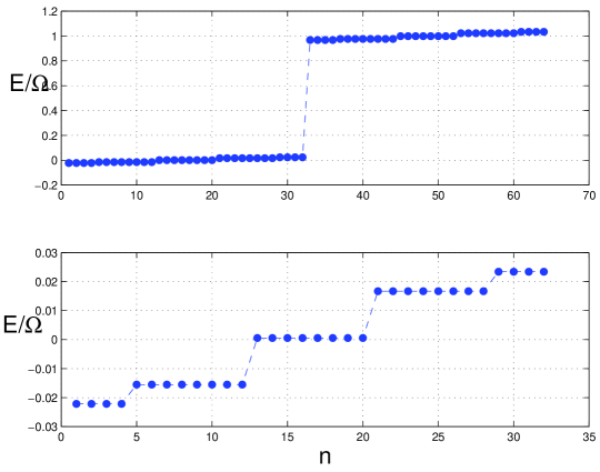
Figure 3. The fine structure pattern of the first Landau level for $\nu=4$, $N_{0}=32$, $\lambda=1/10$.

The finite structure energy gap is not uniform, but a regular pattern emerges looking at sufficiently large $N_{0}/\nu$. The evidence is that the gaps are approximately reproduced by

(14) $$E_{n+1}-E_{n}\propto\sin(n\pi/N_{0})\,,\quad n+\nu/2\equiv 0\mod(2\nu)\,,$$

at least when the degeneracy pattern $\{\nu,2\nu,2\nu,...,2\nu,\nu\}$ is realised. At this level, however, the study is still preliminary.

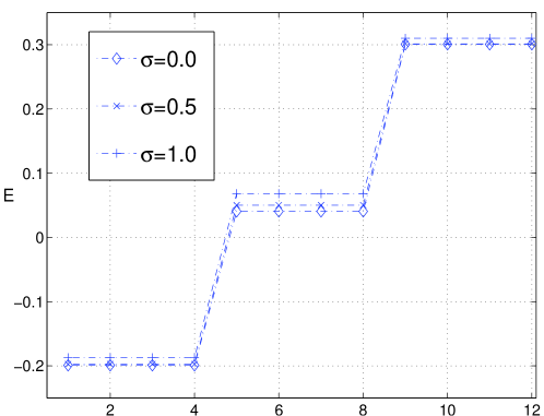
Figure 4. The gaps in the fine structure of the first Landau level under a periodic deformation of the magnetic field, $\nu=4,N_{0}=12$, $\sigma$ is the coupling of the higher harmonic.

6. Concluding remarks

We presented a spectral algorithm which can compute the energy spectrum for a scalar particle on the 2-D flat torus, subject to a transverse magnetic field and any potential energy. To realize the algorithm, it is crucial to implement the correct boundary conditions in order to be able to apply the spectral method based on Fourier transform. The spectrum is typically obtained to a relative error of $10^{-12}$ even on rather coarse meshes. When the field deviates from uniformity in a sinusoidal way, we find a fine structure in the splitting of Landau levels with a regular degeneracy pattern. The problem we considered here originated from the formulation of the Hamiltonian path integral introduced long ago by J.R. Klauder [5]; see also [7]

References

- [1] S. Fubini, “Finite Euclidean magnetic group and theta functions”, Int. J. Mod. Phys., A7, (1992) 4671-4692.
- [2] E. Onofri, “Landau Levels on a torus”, Int. J. Theoret. Phys., 2001, 40, 2, 537–549.
- [3] B. Morariu AND A.P. Polychronakos, “Quantum mechanics on the noncommutative torus”, Nuclear Phys. B, (2001) 610, 3, 531-544
- [4] F. Hirzebruch, “Topologial Methods in Algebraic Geometry”, Springer-Verlag, 1978, 131, Grundlehren der mathematischen Wissenschaften
- [5] J. R. Klauder, “Quantization is Geometry, After All” Annals of Phys. (NY), 188 (1988) 120-130.
- [6] O. Alvarez, “Topological Quantization and Cohomology”, Commun. Math. Phys. 100 (1985), 279–309.
- [7] J.R. Klauder and E. Onofri, “Landau levels and Geometric Quantization”, Int. J. Mod. Phys.”, A4, (1989) 3939.
- [8] M. Frigo and S. G. Johnson The Design and Implementation of FFTW3, Proceedings of the IEEE (2005), 93(2) 216–231
- [9] R. B. Lehoucq, D. C. Sorensen and C. Young, ARPACK Users’ Guide, SIAM, Philadelphia 1998. Matlab’s implementation on R. Radke’s Thesis http://www.caam.rice.edu/software/ARPACK/DOCS/radke.ps.gz.