On The Behavior of Subgradient Projections Methods for Convex Feasibility Problems in Euclidean Spaces

Abstract

We study some methods of subgradient projections for solving a convex feasibility problem with general (not necessarily hyperplanes or half-spaces) convex sets in the inconsistent case and propose a strategy that controls the relaxation parameters in a specific self-adapting manner. This strategy leaves enough user-flexibility but gives a mathematical guarantee for the algorithm’s behavior in the inconsistent case. We present numerical results of computational experiments that illustrate the computational advantage of the new method.

1 Introduction

In this paper we consider, in an Euclidean space framework, the method of simultaneous subgradient projections for solving a convex feasibility problem with general (not necessarily linear) convex sets in the consistent and inconsistent cases. To cope with this situation, we propose two algorithmic developments. One uses steering parameters instead of relaxation parameters in the simultaneous subgradient projection method, and the other is a strategy that controls the relaxation parameters in a specific self-adapting manner that leaves enough user-flexibility while yielding some mathematical guarantees for the algorithm’s behavior in the inconsistent case. For the algorithm that uses steering parameters there is currently no mathematical theory. We present numerical results of computational experiments that show the computational advantage of the mathematically-founded algorithm implementing our specific relaxation strategy. In the remainder of this section we elaborate upon the meaning of the above-made statements.

Given $m$ closed convex subsets $Q_{1},Q_{2},\cdots,Q_{m}\subseteq R^{n}$ of the $n$-dimensional Euclidean space, expressed as

$$Q_{i}=\left\{x\in R^{n}\mid f_{i}(x)\leq 0\right\},$$ (1.1)

where $f_{i}:R^{n}\rightarrow R$ is a convex function, the convex feasibility problem (CFP) is

$$\text{find a point }x^{\ast}\in Q:=\cap_{i=1}^{m}Q_{i}.$$ (1.2)

As is well-known, if the sets are given in any other form then they can be represented in the form (1.1) by choosing for $f_{i}$ the squared Euclidean distance to the set. Thus, it is required to solve the system of convex inequalities

$$\text{ }f_{i}(x)\leq 0,\text{ \ \ }i=1,2,\ldots,m.$$ (1.3)

A fundamental question is how to approach the CFP in the inconsistent case, when $Q=\cap_{i=1}^{m}Q_{i}=\emptyset.$ Logically, algorithms designed to solve the CFP by finding a point $x^{\ast}\in Q$ are bound to fail and should, therefore, not be employed. But this is not always the case. Projection methods that are commonly used for the CFP, particularly in some very large real-world applications (see details below) are applied to CFPs without prior knowledge whether or not the problem is consistent. In such circumstances it is imperative to know how would a method, that is originally known to converge for a consistent CFP, behave if consistency is not guaranteed.

We address this question for a particular type of projection methods. In general, sequential projection methods exhibit cyclic convergence in the inconsistent case. This means that the whole sequence of iterates does not converge, but it breaks up into $m$ convergent subsequences (see Gubin, Polyak and Raik [34, Theorem 2] and Bauschke, Borwein and Lewis [5]). In contrast, simultaneous projection methods generally converge, even in the inconsistent case, to a minimizer of a proximity function that “measures” the weighted sum of squared distances to all sets of the CFP, provided such a minimizer exists (see Iusem and De Pierro [37] for a local convergence proof and Combettes [26] for a global one).

Therefore, there is an advantage in using simultaneous projection methods from the point of view of convergence. Additional advantages are that (i) they are inherently parallel already at the mathematical formulation level due to the simultaneous nature, and (ii) they allow the user to assign weights (of importance) to the sets of the CFP. However, a severe limitation, common to sequential as well as simultaneous projection methods, is the need to solve an inner-loop distance-minimization step for the calculation of the orthogonal projection onto each individual set of the CFP. This need is alleviated only for convex sets that are simple to project onto, such as hyperplanes or half-spaces.

A useful path to circumvent this limitation is to use subgradient projections that rely on calculation of subgradients at the current (available) iteration points, see Censor and Lent [20] or [21, Section 5.3]. Iusem and Moledo [41] studied the simultaneous projection method with subgradient projections but only for consistent CFPs. To the best of our knowledge, there does not exist a study of the simultaneous projection method with subgradient projections for the inconsistent case. Our present results are a contribution towards this goal.

The CFP is a fundamental problem in many areas of mathematics and the physical sciences, see, e.g., Combettes [25, 27] and references therein. It has been used to model significant real-world problems in image reconstruction from projections, see, e.g., Herman [35], in radiation therapy treatment planning, see Censor, Altschuler and Powlis [17] and Censor [15], and in crystallography, see Marks, Sinkler and Landree [42], to name but a few, and has been used under additional names such as set-theoretic estimation or the feasible set approach. A common approach to such problems is to use projection algorithms, see, e.g., Bauschke and Borwein [4], which employ orthogonal projections (i.e., nearest point mappings) onto the individual sets $Q_{i}.$ The orthogonal projection $P_{\Omega}(z)$ of a point $z\in R^{n}$ onto a closed convex set $\Omega\subseteq R^{n}$ is defined by

$$P_{\Omega}(z):=\operatorname{argmin}\{\parallel z-x\text{ }\|\mid\text{ }x\in\Omega\},$$ (1.4)

where, throughout this paper, $\parallel\cdot\parallel$ and $\left\langle\cdot,\cdot\right\rangle$ denote the Euclidean norm and inner product, respectively, in $R^{n}.$ Frequently a relaxation parameter is introduced so that

$$P_{\Omega,\lambda}(z):=(1-\lambda)z+\lambda P_{\Omega}(z)$$ (1.5)

is the relaxed projection of $z$ onto $\Omega$ with relaxation $\lambda.$ Many iterative projection algorithms for the CFP were developed, see Subsection 1.1 below.

1.1 Projection methods: Advantages and earlier work

The reason why the CFP is looked at from the viewpoint of projection methods can be appreciated by the following brief comments, that we made in earlier publications, regarding projection methods in general. Projections onto sets are used in a variety of methods in optimization theory but not every method that uses projections really belongs to the class of projection methods. Projection methods are iterative algorithms which use projections onto sets. They rely on the general principle that projections onto the given individual sets are easier to perform then projections onto other sets derived from the given individual sets (intersections, image sets under some transformation, etc.)

A projection algorithm reaches its goal, related to the whole family of sets, by performing projections onto the individual sets. Projection algorithms employ projections onto convex sets in various ways. They may use different kinds of projections and, sometimes, even use different types of projections within the same algorithm. They serve to solve a variety of problems which are either of the feasibility or the optimization types. They have different algorithmic structures, of which some are particularly suitable for parallel computing, and they demonstrate nice convergence properties and/or good initial behavior patterns.

Apart from theoretical interest, the main advantage of projection methods, which makes them successful in real-world applications, is computational. They commonly have the ability to handle huge-size problems that are beyond the ability of more sophisticated, currently available, methods. This is so because the building blocks of a projection algorithm are the projections onto the given individual sets (which are easy to perform) and the algorithmic structure is either sequential or simultaneous (or in-between).

The field of projection methods is vast and we mention here only a few recent works that can give the reader some good starting points. Such a list includes, among many others, the works of Crombez [29, 30], the connection with variational inequalities, see, e.g., Aslam-Noor [43], Yamada [48] which is motivated by real-world problems of signal processing, and the many contributions of Bauschke and Combettes, see, e.g., Bauschke, Combettes and Kruk [6] and references therein. Bauschke and Borwein [4] and Censor and Zenios [21, Chapter 5] provide reviews of the field.

Systems of linear equations, linear inequalities, or convex inequalities are all encompassed by the CFP which has broad applicability in many areas of mathematics and the physical and engineering sciences. These include, among others, optimization theory (see, e.g., Eremin [33], Censor and Lent [20] and Chinneck [22]), approximation theory (see, e.g., Deutsch [31] and references therein), image reconstruction from projections in computerized tomography (see, e.g., Herman [35, 36]) and control theory (see, e.g., Boyd et al. [8].)

Combettes [28] and Kiwiel [40] have studied the subgradient projection method for consistent CFPs. Their work presents more general algorithmic steps and is formulated in Hilbert space. Some work has already been done on detecting infeasibility with certain subgradient projection methods by Kiwiel [38, 39]. However, our approach differs from the latter in that it aims at a subgradient projection method that “will work” regardless of the feasibility of the underlying CFP and which does not require the user to study in advance whether or not the CFP is consistent. Further questions arise such as that of combining our work, or the above quoted results, with Pierra’s [45] product space formalism, as extended to handle inconsistent situations by Combettes [26]. These questions are currently under investigation.

2 Simultaneous subgradient projections with steering parameters

Subgradient projections have been incorporated in iterative algorithms for the solution of CFPs. The cyclic subgradient projections (CSP) method for the CFP was given by Censor and Lent [20] as follows.

Algorithm 2.1

The method of cyclic subgradient projections (CSP).

Initialization: $x^{0}\in R^{n}$ is arbitrary.

Iterative step: Given $x^{k},$ calculate the next iterate $x^{k+1}$ by

$$x^{k+1}=\left\{\begin{array}[c]{ll}x^{k}-\alpha_{k}\frac{\displaystyle f_{i(k)}(x^{k})}{\displaystyle\parallel\;t^{k}\parallel^{2}}t^{k},&\mathrm{if}\;\;f_{i(k)}(x^{k})>0,\\ x^{k},&\mathrm{if}\;\;f_{i(k)}(x^{k})\leq 0,\end{array}\right.$$ (2.1)

where $t^{k}\in\partial f_{i(k)}(x^{k})$ is a subgradient of $f_{i(k)}$ at the point $x^{k}$, and the relaxation parameters $\{\alpha_{k}\}_{k=0}^{\infty}$ are confined to an interval $\epsilon_{1}\leq\alpha_{k}\leq 2-\epsilon_{2}$, for all $k\geq 0$, with some, arbitrarily small, $\epsilon_{1},\epsilon_{2}>0.$

Control: Denoting $I:=\{1,2,\ldots,m\},$ the sequence $\{i(k)\}_{k=0}^{\infty}$ is an almost cyclic control sequence on $I$. This means (see, e.g., [21, Definition 5.1.1]) that $i(k)\in I$ for all $k\geq 0$ and there exists an integer $C\geq m$ such that, for all $k\geq 0$, $I\subseteq\{i(k+1),i(k+2),\ldots,i(k+C)\}.$

Observe that if $t^{k}=0$, then $f_{i(k)}$ takes its minimal value at $x^{k}$, implying, by the nonemptiness of $Q$, that $f_{i(k)}(x^{k})\leq 0$, so that $x^{k+1}=x^{k}$. Relations of the CSP method to other iterative methods for solving the convex feasibility problem and to the relaxation method for solving linear inequalities can be found, e.g., in [21, Chapter 5], see also, Bauschke and Borwein [4, Section 7]. Since sequential projection methods for CFPs commonly have fully-simultaneous counterparts, the simultaneous subgradient projections (SSP) method of Dos Santos [32] and Iusem and Moledo [41] is a natural algorithmic development.

Algorithm 2.2

The method of simultaneous subgradient projections (SSP).

Initialization: $x^{0}\in R^{n}$ is arbitrary.

Iterative step: (i) Given $x^{k},$ calculate, for all $i\in I=\{1,2,\ldots,m\},$ intermediate iterates $y^{k+1,i}$ by

$$y^{k+1,i}=\left\{\begin{array}[c]{ll}x^{k}-\alpha_{k}\frac{\displaystyle f_{i}(x^{k})}{\displaystyle\parallel\;t^{k}\parallel^{2}}t^{k},&\mathrm{if}\;\;f_{i}(x^{k})>0,\\ x^{k},&\mathrm{if}\;\;f_{i}(x^{k})\leq 0,\end{array}\right.$$ (2.2)

where $t^{k}\in\partial f_{i}(x^{k})$ is a subgradient of $f_{i}$ at the point $x^{k}$, and the relaxation parameters $\{\alpha_{k}\}_{k=0}^{\infty}$ are confined to an interval $\epsilon_{1}\leq\alpha_{k}\leq 2-\epsilon_{2}$, for all $k\geq 0$, with some, arbitrarily small, $\epsilon_{1},\epsilon_{2}>0.$

(ii) Calculate the next iterate $x^{k+1}$ by

$$x^{k+1}=\sum_{i=1}^{m}w_{i}y^{k+1,i}$$ (2.3)

where $w_{i}$ are fixed, user-chosen, positive weights with $\sum_{i=1}^{m}w_{i}=1.$

The convergence analysis for this algorithm is currently available only for consistent ($Q\neq\emptyset$) CFPs, see [32, 41]. In our experimental work, reported in the sequel, we applied Algorithm 2.2 to CFPs without knowing whether or not they are consistent. Convergence is diagnosed by performing plots of a proximity function that measures in some manner the infeasibility of the system. We used the weighted proximity function of the form

$$p(x):=(1/2)\sum_{i=1}^{m}w_{i}\parallel P_{i}(x)-x\parallel^{2}$$ (2.4)

were $P_{i}(x)$ is the orthogonal projection of the point $x$ onto $Q_{i}.$ To combat instabilities in those plots that appeared occasionally in our experiments we used steering parameters $\sigma_{k}$ instead of the relaxation parameters $\alpha_{k}$ in Algorithm 2.2. To this end we need the following definition.

Definition 2.3

A sequence $\{\sigma_{k}\}_{k=0}^{\infty}$ of real numbers $0\leq\sigma_{k}<1$ is called a steering sequence if it satisfies the following conditions:

$$\lim_{k\rightarrow\infty}\sigma_{k}=0,$$ (2.5)

$$\sum_{k=0}^{\infty}\sigma_{k}=+\infty,$$ (2.6)

$$\sum_{k=0}^{\infty}\mid\sigma_{k}-\sigma_{k+m}\mid<+\infty.$$ (2.7)

A historical and technical discussion of these conditions can be found in [3]. The sequential and simultaneous Halpern-Lions-Wittmann-Bauschke (HLWB) algorithms discussed in Censor [16] employ the parameters of a steering sequence to “force” (steer) the iterates towards the solution of the best approximation problem (BAP). This steering feature of the steering parameters has a profound effect on the behavior of any sequence of iterates $\{x^{k}\}_{k=0}^{\infty}$. We return to this point in Section 6.

Algorithm 2.4

The method of simultaneous subgradient projections (SSP) with steering.

Initialization: $x^{0}\in R^{n}$ is arbitrary.

Iterative step: (i) Given $x^{k},$ calculate, for all $i\in I=\{1,2,\ldots,m\},$ intermediate iterates $y^{k+1,i}$ by

$$y^{k+1,i}=\left\{\begin{array}[c]{ll}x^{k}-\sigma_{k}\frac{\displaystyle f_{i}(x^{k})}{\displaystyle\parallel\;t^{k}\parallel^{2}}t^{k},&\mathrm{if}\;\;f_{i}(x^{k})>0,\\ x^{k},&\mathrm{if}\;\;f_{i}(x^{k})\leq 0,\end{array}\right.$$ (2.8)

where $t^{k}\in\partial f_{i}(x^{k})$ is a subgradient of $f_{i}$ at the point $x^{k}$, and $\{\sigma_{k}\}_{k=0}^{\infty}$ is a sequence of steering parameters.

(ii) Calculate the next iterate $x^{k+1}$ by

$$x^{k+1}=\sum_{i=1}^{m}w_{i}y^{k+1,i}$$ (2.9)

where $w_{i}$ are fixed, user-chosen, positive weights with $\sum_{i=1}^{m}w_{i}=1.$

3 Subgradient projections with strategical relaxation: Preliminaries

Considering the CFP (1.2), the envelope of the family of functions $\{f_{i}\}_{i=1}^{m}$ is the function

$$f(x):=\max\{f_{i}(x)\mid i=1,2,\ldots,m\}$$ (3.1)

which is also convex. Clearly, the consistent CFP is equivalent to finding a point in

$$Q=\cap_{i=1}^{m}Q_{i}=\{x\in R^{n}\mid f(x)\leq 0\}.$$ (3.2)

The subgradient projections algorithmic scheme that we propose here employs a strategy for controlling the relaxation parameters in a specific manner, leaving enough user-flexibility while giving some mathematical guarantees for the algorithm’s behavior in the inconsistent case. It is described as follows:

Algorithm 3.1

Initialization: Let $M$ be a positive real number and let $x^{0}\in R^{n}$ be any initial point.

Iterative step: Given the current iterate $x^{k},$ set

$$I(x^{k}):=\{i\mid 1\leq i\leq m\text{ \ and \ }f_{i}(x^{k})=f(x^{k})\}$$ (3.3)

and choose a nonnegative vector $w^{k}=(w_{1}^{k},w_{2}^{k},\ldots,w_{m}^{k})\in R^{m}$ such that

$$\sum_{i=1}^{m}w_{i}^{k}=1\text{ \ and \ }w_{i}^{k}=0\text{ \ if \ }i\notin I(x^{k}).\text{}$$ (3.4)

Let $\lambda_{k}$ be any nonnegative real number such that

$$\max\left(0,\text{ }f(x^{k})\right)\leq\lambda_{k}M^{2}\leq 2\max\left(0,\text{ }f(x^{k})\right)$$ (3.5)

and calculate

$$x^{k+1}=x^{k}-\lambda_{k}\sum_{i\in I(x^{k})}w_{i}^{k}\xi_{i}^{k},$$ (3.6)

where, for each $i\in I(x^{k}),$ we take a subgradient $\xi_{i}^{k}\in\partial f_{i}(x^{k}).\vskip 6.0pt plus 2.0pt minus 2.0pt$

It is interesting to note that any sequence $\left\{x^{k}\right\}_{k=0}^{\infty}$ generated by this algorithm is well-defined, no matter how $x^{0}$ and $M$ are chosen. Similarly to other algorithms described above, Algorithm 3.1 requires computing subgradients of convex functions. In case a function is differentiable, this reduces to gradient calculations. Otherwise, one can use the subgradient computing procedure presented in Butnariu and Resmerita [12].

The procedure described above was previously studied in Butnariu and Mehrez [11]. The main result there shows that the procedure converges to a solution of the CFP under two conditions: (i) that the solution set $Q$ has nonempty interior and (ii) that the envelope $f$ is uniformly Lipschitz on $R^{n},$ that is, there exists a positive real number $L$ such that

$$\left|f(x)-f(y)\right|\leq L\left\|x-y\right\|,\text{ \ for all \ }x,y\in R^{n}.$$ (3.7)

Both conditions (i) and (ii) are restrictive and it is difficult to verify their validity in practical applications. In the following we show that this method converges to solutions of consistent CFPs under less demanding conditions. In fact, we show that if the solution set $Q$ of the given CFP has nonempty interior, then convergence of Algorithm 3.1 to a point in $Q$ is ensured even if the function $f$ is not uniformly Lipschitz on $R^{n}$ (i.e., even if $f$ does not satisfy condition (ii) above). However, verifying whether $\operatorname{int}Q\neq\varnothing$ prior to solving a CFP may be difficult or even impossible. Therefore, it is desirable to have alternative conditions, which may be easier to verify in practice, that can ensure convergence of our algorithm to solutions of the CFP, provided that such solutions exist. This is why we prove convergence of Algorithm 3.1 to solutions of consistent CFPs whenever the envelope $f$ of the functions $f_{i}$ involved in the given CFP is strictly convex. Strict convexity of the envelope function $f$ associated with a consistent CFP implies that either the solution set $Q$ of the CFP is a singleton, in which case $\operatorname{int}Q=\varnothing$, or that $Q$ contains (at least) two different solutions of the CFP implying that int $Q\neq\varnothing$. Verification of whether $Q$ is a singleton or not is as difficult as deciding whether int $Q\neq\varnothing$. By contrast, since $f$ is strictly convex whenever each $f_{i}$ is strictly convex, verification of strict convexity of $f$ may be relatively easily done in some situations of practical interest, such as when each $f_{i}$ is a quadratic convex function. In the latter case, strict convexity of $f_{i}$ amounts to positive definiteness of the matrix of its purely quadratic part.

It is interesting to note in this context that when the envelope $f$ of the CFP is not strictly convex one may consider a “regularized” CFP in which each $f_{i}$ which is not strictly convex is replaced by

$$\overline{f_{i}}(x):=f_{i}(x)+\alpha\|x\|^{2}$$ (3.8)

for some positive real number $\alpha.$ Clearly, all $\overline{f_{i}}$ are strictly convex and, thus, so is the envelope $\overline{f}$ of the regularized problem. Therefore, if the regularized problem has solutions, then our Algorithm 3.1 will produce approximations of such solutions. Moreover, any solution of the regularized problem is a solutions of the original problem and, thus, by solving the regularized problem we implicitly solve the original problem. The difficult part of this approach is that, even if the original CFP is consistent then the regularized version of it may be inconsistent for all, or for some, values $\alpha>0.$ How to decide whether an $\alpha>0$ exists such that the corresponding regularized CFP is consistent and how to compute such an $\alpha$ (if any) are questions whose answers we do not know.

4 Subgradient projections with strategical relaxation: convergence analysis

In order to discuss the convergence behavior of the subgradient projections method with strategical relaxation, recall that convex functions defined on the whole space $R^{n}$ are continuous and, consequently, are bounded on bounded sets in $R^{n}$. Therefore, the application of Butnariu and Iusem [10, Proposition 1.1.11] or Bauschke and Borwein [4, Proposition 7.8] to the convex function $f$ shows that it is Lipschitz on bounded subsets of $R^{n},$ i.e., for any nonempty bounded subset $S\subseteq R^{n}$ there exists a positive real number $L(S),$ called a Lipschitz constant of $f$ over the set $S,$ such that

$$\left|f(x)-f(y)\right|\leq L(S)\left\|x-y\right\|,\text{ for all \ }x,y\in S.$$ (4.1)

Our next result is a convergence theorem for Algorithm 3.1 when applied to a consistent CFP. It was noted in the previous section that Algorithm 3.1 is well-defined regardless of how the initial point $x^{0}$ or the positive constant $M$ involved in the algorithm are chosen. However, this is no guarantee that a sequences $\{x_{k}\}_{k=0}^{\infty}$ generated by Algorithm 3.1 for random choices of $x^{0}$ and $M$ will converge to solutions of the CFP, even if such solutions exist. The theorem below shows a way of choosing $x^{0}$ and $M$ which ensures that, under some additional conditions for the problem data, the sequence $\{x_{k}\}_{k=0}^{\infty}$ generated by Algorithm 3.1 will necessarily approximate a solution of the CFP (provided that solutions exist). As shown in Section 5 below, determining $x^{0}$ and $M$ as required in the next theorem can be quite easily done for practically significant classes of CFPs. Also, as shown in Section 6, determining $x^{0}$ and $M$ in this manner, enhances the self-adaptability of the procedure to the problem data and makes Algorithm 3.1 produce approximations of solutions of the CFP which, in many cases, are more accurate than those produced by other CFP solving algorithms.

Theorem 4.1

If a positive number $M$ and an initial point $x^{0}$ in Algorithm 3.1 are chosen so that $M\geq L(B(x^{0},r))$ for some positive real number $r$ satisfying the condition

$$B(x^{0},r/2)\cap Q\neq\emptyset,$$ (4.2)

and if at least one of the following conditions holds:

(i) $B(x^{0},r/2)\cap\operatorname*{int}\,Q\neq\emptyset,$

(ii) the function $f$ is strictly convex,
then any sequence $\left\{x^{k}\right\}_{k=0}^{\infty},$ generated by Algorithm 3.1, converges to an element of $Q.\vskip 3.0pt plus 1.0pt minus 1.0pt$

We present the proof of Theorem 4.1 as a sequence of lemmas. To do so, note that if $\left\{x^{k}\right\}_{k=0}^{\infty}$ is generated by Algorithm 3.1 then for each integer $k\geq 0,$ we have

$$x^{k+1}=x^{k}-\lambda_{k}\nu^{k},$$ (4.3)

where

$$\nu^{k}:=\sum_{i\in I(x^{k})}w_{i}^{k}\xi_{i}^{k}\in\operatorname*{conv}\cup_{i\in I(x^{k})}\partial f_{i}(x^{k}).$$ (4.4)

Using (4.3), for any $z\in R^{n},$ we have

$$\left\|x^{k+1}-z\right\|^{2}=\left\|x^{k}-z\right\|^{2}+\lambda_{k}\left(\lambda_{k}\left\|\nu^{k}\right\|^{2}-2\left\langle\nu^{k},x^{k}-z\right\rangle\right).$$ (4.5)

By Clarke [24, Proposition 2.3.12] we deduce that

$$\partial f(x^{k})=\operatorname*{conv}\cup_{i\in I(x^{k})}\partial f_{i}(x^{k})$$ (4.6)

and this implies that $\nu^{k}\in\partial f(x^{k})$ because of (4.4). Therefore,

$$\left\langle\nu^{k},z-x^{k}\right\rangle\leq f_{+}^{\prime}(x^{k};z-x^{k})$$ (4.7)

where $f_{+}^{\prime}(u;v)$ denotes the right-sided directional derivative at $u$ in the direction $v.$ Now suppose that $M,$ $r$ and $x^{0}$ are chosen according to the requirements of Theorem 4.1, that is,

$$r>0\text{, \ }M\geq L(B(x^{0},r))\text{ and }B(x^{0},r/2)\cap Q\neq\emptyset.$$ (4.8)

Next we prove the following basic fact.

Lemma 4.2

If (4.8) is satisfied and if $z\in B(x^{0},r/2)\cap Q,$ then for all $k\geq 0$, we have for any sequence $\left\{x^{k}\right\}_{k=0}^{\infty},$ generated by Algorithm 3.1,

$$x^{k+1}\in B(x^{0},r)\text{ and }\left\|x^{k+1}-z\right\|\leq\left\|x^{k}-z\right\|\leq r/2\text{.}$$ (4.9)

Proof. We first show that if, for some integer $k\geq 0$,

$$x^{k}\in B(x^{0},r)\text{ and }\left\|x^{k}-z\right\|\leq r/2$$ (4.10)

then (4.9) holds. If $\lambda_{k}=0$ or $\nu^{k}=0,$ then, by (4.3), we have $x^{k+1}=x^{k}$ which, combined with (4.10), implies (4.9). Assume now that $\lambda_{k}\neq 0$ and $\nu^{k}\neq 0.$ Since, by (4.10), $x^{k}\in B(x^{0},r),$ by (4.8) and by [24, Proposition 2.1.2(a)], we deduce that

$$M\geq L(B(x^{0},r))\geq\left\|\nu^{k}\right\|.$$ (4.11)

According to (3.5), we also have $f(x^{k})>0$ (otherwise $\lambda_{k}=0$). Since $f(z)\leq 0$ we obtain from the subgradient inequality

$$\left\langle\nu^{k},x^{k}-z\right\rangle\geq f(x^{k})-f(z)\geq f(x^{k})>0.$$ (4.12)

This and (4.11) imply

$$2\left\langle\nu^{k},x^{k}-z\right\rangle\geq 2f(x^{k})\geq\lambda_{k}M^{2}\geq\lambda_{k}\left\|\nu^{k}\right\|^{2},$$ (4.13)

showing that the quantity inside the parentheses in (4.5) is nonpositive. Thus, we deduce that

$$\left\|x^{k+1}-z\right\|\leq\left\|x^{k}-z\right\|\leq r/2$$ (4.14)

in this case too. This proves that if (4.10) is true for all $k\geq 0$, then so is (4.9). Now, we prove by induction that (4.10) is true for all $k\geq 0$. If $k=0$ then (4.10) obviously holds. Suppose that (4.10) is satisfied for some $k=p.$ As shown above, this implies that condition (4.9) is satisfied for $k=p$ and, thus, we have that

$$x^{p+1}\in B(x^{0},r)\text{ and }\left\|x^{p+1}-z\right\|\leq r/2.$$ (4.15)

Hence, condition (4.10) also holds for $k=p+1.$ Consequently, condition (4.9) holds for $k=p+1$ and this completes the proof.   

Observe that, according to Lemma 4.2, if $\left\{x^{k}\right\}_{k=0}^{\infty}$ is a sequence generated by Algorithm 3.1 and if the conditions (4.8) are satisfied, then there exists $z\in B(x^{0},r/2)\cap Q$ and for any such $z$ the sequence $\left\{\left\|x^{k}-z\right\|\right\}_{k=0}^{\infty}$ is nonincreasing and bounded from below and, therefore, convergent. Since the sequence $\left\{\left\|x^{k}-z\right\|\right\}_{k=0}^{\infty}$ is convergent it is also bounded and, consequently, the sequence $\left\{x^{k}\right\}_{k=0}^{\infty}$ is bounded too. This shows that the next result applies to any sequence $\left\{x^{k}\right\}_{k=0}^{\infty}$ generated by Algorithm 3.1 under the assumptions of Theorem 4.1.

Lemma 4.3

If $\left\{x^{k}\right\}_{k=0}^{\infty}$ is a bounded sequence generated by Algorithm 3.1, then the sequence $\left\{x^{k}\right\}_{k=0}^{\infty}$ has accumulation points and for each accumulation point $x^{\ast}$ of $\left\{x^{k}\right\}_{k=0}^{\infty}$ there exists a sequence of natural numbers $\left\{k_{s}\right\}_{s=0}^{\infty}$ such that the following limits exist

$$x^{\ast} =\lim_{s\rightarrow\infty}x^{k_{s}},\text{ }\lambda_{\ast}=\lim_{s\rightarrow\infty}\lambda_{k_{s}},$$ (4.16)

$$\xi_{i}^{\ast} =\lim_{s\rightarrow\infty}\xi_{i}^{k_{s}},\text{ }w_{i}^{\ast}=\lim_{s\rightarrow\infty}w_{i}^{k_{s}},\text{ for all }i=1,2,\ldots,m,$$ (4.17)

$$\nu^{\ast} =\lim_{s\rightarrow\infty}\nu^{k_{s}},$$ (4.18)

and we have

$$w^{\ast}:=(w_{1}^{\ast},w_{2}^{\ast},\ldots,w_{m}^{\ast})\in R_{+}^{m}\ \text{and }\sum_{i\in I(x^{\ast})}w_{i}^{\ast}=1$$ (4.19)

and

$$\nu^{\ast}=\sum_{i\in I(x^{\ast})}w_{i}^{\ast}\xi_{i}^{\ast}\in\partial f(x^{\ast}).$$ (4.20)

Moreover, if $\lambda_{\ast}=0,$ then $x^{\ast}$ is a solution of the CFP.

Proof. The sequence $\left\{x^{k}\right\}_{k=0}^{\infty}$ is bounded and, thus, has accumulation points. Let $x^{\ast}$ be an accumulation point of $\left\{x^{k}\right\}_{k=0}^{\infty}$ and let $\left\{x^{p_{s}}\right\}_{s=0}^{\infty}$ be a convergent subsequence of $\left\{x^{k}\right\}_{k=0}^{\infty}$ such that $x^{\ast}=\lim_{s\rightarrow\infty}x^{p_{s}}.$ The function $f$ is continuous (since it is real-valued and convex on $R^{n}$), hence, it is bounded on bounded subsets of $R^{n}$. Therefore, the sequence $\left\{f(x^{p_{s}})\right\}_{s=0}^{\infty}$ converges to $f(x^{\ast})$ and the sequence $\left\{f(x^{k})\right\}_{k=0}^{\infty}$ is bounded. By (3.5), boundedness of $\left\{f(x^{k})\right\}_{k=0}^{\infty}$ implies that the sequence $\left\{\lambda_{k}\right\}_{k=0}^{\infty}$ is bounded. Since, for every $i=1,2,\ldots,m,$ the operator $\partial f_{i}:R^{n}\rightarrow 2^{R^{n}}$ is monotone, it is locally bounded (cf. Pascali and Sburlan [44, Theorem on p. 104]).

Consequently, there exists a neighborhood $U$ of $x^{\ast}$ on which all $\partial f_{i},$ $i=1,2,\ldots,m,$ are bounded. Clearly, since $x^{\ast}=\lim_{s\rightarrow\infty}x^{p_{s}}$, the neighborhood $U$ contains all but finitely many terms of the sequence $\left\{x^{p_{s}}\right\}_{s=0}^{\infty}.$ This implies that the sequences $\left\{\xi_{i}^{p_{s}}\right\}_{s=0}^{\infty}$ are uniformly bounded and, therefore, the sequence $\left\{\nu^{p_{s}}\right\}_{s=0}^{\infty}$ is bounded too.

Therefore, there exist a subsequence $\left\{k_{s}\right\}_{s=0}^{\infty}$ of $\left\{p_{s}\right\}_{s=0}^{\infty}$ such that the limits in (4.16)–(4.18) exist. Obviously, the vector $w^{\ast}=(w_{1}^{\ast},w_{2}^{\ast},\ldots,w_{m}^{\ast})\in R_{+}^{m},$ and, according to [11, Lemma 1], we also have $\sum_{i\in I(x^{\ast})}w_{i}^{\ast}=1$. This and (4.4) imply that $\nu^{\ast}=\sum_{i\in I(x^{\ast})}w_{i}^{\ast}\xi_{i}^{\ast}.$

Observe that, since $\nu^{k_{s}}\in\partial f(x^{k_{s}})$ for all $s\geq 0$, and since $\partial f$ is a closed mapping (cf. Phelps [46, Proposition 2.5]), we have that $\nu^{\ast}\in\partial f(x^{\ast}).$ Now, if $\lambda_{\ast}=0$ then, according to (3.5), and the continuity of $f,$ we deduce

$$0\leq\max\{0,f(x^{\ast})\}=\lim_{s\rightarrow\infty}\max\{0,f(x^{k_{s}})\}\leq\lim_{s\rightarrow\infty}\lambda_{k_{s}}M^{2}=\lambda_{\ast}M^{2}=0,$$ (4.21)

which implies that $f(x^{\ast})\leq 0$, that is, $x^{\ast}\in Q.$   

Lemma 4.4

Let $\left\{x^{k}\right\}_{k=0}^{\infty}$ be a sequence generated by Algorithm 3.1. If (4.8) is satisfied and if at least one of the conditions (i) or (ii) of Theorem 4.1 holds, then the sequence $\left\{x^{k}\right\}_{k=0}^{\infty}$ has accumulation points and any such point belongs to $Q.\vskip 3.0pt plus 1.0pt minus 1.0pt$

Proof. As noted above, when (4.8) is satisfied then the sequence $\left\{x^{k}\right\}_{k=0}^{\infty}$ is bounded and, hence, it has accumulation points. Let $x^{\ast}$ be such an accumulation point and let $\left\{k_{s}\right\}_{s=0}^{\infty}$ be the sequence of natural numbers associated with $x^{\ast}$ whose existence is guaranteed by Lemma 4.3. Since, for any $z\in C\cap B(x^{0},r/2),$ the sequence $\left\{\left\|x^{k}-z\right\|\right\}_{k=0}^{\infty}$ is convergent (cf. Lemma 4.2) we deduce that

$$\left\|x^{\ast}-z\right\| =\lim_{s\rightarrow\infty}\left\|x^{k_{s}}-z\right\|=\lim_{k\rightarrow\infty}\left\|x^{k}-z\right\|=\lim_{s\rightarrow\infty}\left\|x^{k_{s}+1}-z\right\|$$ (4.22)

$$=\left\|x^{\ast}-\lambda_{\ast}\nu^{\ast}-z\right\|.$$

This implies

$$\left\|x^{\ast}-z\right\|^{2}=\left\|x^{\ast}-z\right\|^{2}+\lambda_{\ast}\left(\lambda_{\ast}\left\|\nu^{\ast}\right\|^{2}-2\left\langle\nu^{\ast},x^{\ast}-z\right\rangle\right).$$ (4.23)

If $\lambda_{\ast}=0,$ then $x^{\ast}\in Q$ by Lemma 4.3. Suppose that $\lambda_{\ast}>0.$ Then, by (4.23), we have

$$\lambda_{\ast}\left\|\nu^{\ast}\right\|^{2}-2\left\langle\nu^{\ast},x^{\ast}-z\right\rangle=0,$$ (4.24)

for all $z\in C\cap B(x^{0},r/2).$ We distinguish now between two possible cases.

Case I: Assume that condition (i) of Theorem 4.1 is satisfied. According to (4.24), the set $Q\cap B(x^{0},r/2)$ is contained in the hyperplane

$$H:=\left\{x\in R^{n}\mid\left\langle\nu^{\ast},x\right\rangle=(1/2)\left(2\left\langle\nu^{\ast},x^{\ast}\right\rangle-\lambda_{\ast}\left\|\nu^{\ast}\right\|^{2}\right)\right\}.$$ (4.25)

By condition (i) of Theorem 4.1, it follows that $\mathrm{\operatorname*{int}}\,\left(Q\cap B(x^{0},r/2)\right)\neq\emptyset$ and this is an open set contained in $\mathrm{\operatorname*{int}}\,H.$ So, unless $\nu^{\ast}=0$ (in which case $H=R^{n}$), we have reached a contradiction because $\mathrm{\operatorname*{int}}\,H=\emptyset.$ Therefore, we must have $\nu^{\ast}=0.$ According to Lemma 4.3, we have $0=\nu^{\ast}\in\partial f(x^{\ast})$ which implies that $x^{\ast}$ is a global minimizer of $f.$ Consequently, for any $z\in Q$ we have $f(x^{\ast})\leq f(z)\leq 0,$ that is, $x^{\ast}\in Q.$

Case II: Assume that condition (ii) of Theorem 4.1 is satisfied. According to (4.24), we have

$$\lambda_{\ast}\left\|\nu^{\ast}\right\|^{2}=2\left\langle\nu^{\ast},x^{\ast}-z\right\rangle.$$ (4.26)

By (3.5), the definition of $M$ and [24, Proposition 2.1.2] we deduce that

$$2f(x^{k_{s}})\geq\lambda_{k_{s}}M^{2}\geq\lambda_{k_{s}}\left\|\nu^{k_{s}}\right\|^{2},$$ (4.27)

for all integers $s\geq 0$. Letting $s\rightarrow\infty$ we get

$$2f(x^{\ast})\geq\lambda_{\ast}M^{2}\geq\lambda_{\ast}\left\|\nu^{\ast}\right\|^{2}=2\left\langle\nu^{\ast},x^{\ast}-z\right\rangle,$$ (4.28)

where the last equality follows from (4.26). Consequently, we have

$$f(x^{\ast})\geq\left\langle\nu^{\ast},x^{\ast}-z\right\rangle,\text{ \ \ for all \ \ }z\in Q\cap B(x^{0},r/2).$$ (4.29)

Convexity of $f$ implies that, for all $z\in Q\cap B(x^{0},r/2),$

$$-f(x^{\ast})\leq\left\langle\nu^{\ast},z-x^{\ast}\right\rangle\leq f(z)-f(x^{\ast})\leq-f(x^{\ast}).$$ (4.30)

Therefore, we have that

$$-f(x^{\ast})=\left\langle\nu^{\ast},z-x^{\ast}\right\rangle=f(z)-f(x^{\ast}),\text{ for all \ \ }z\in Q\cap B(x^{0},r/2).$$ (4.31)

Thus $f(z)=0,$ for all $z\in Q\cap B(x^{0},r/2).$ Hence, using again the convexity of $f,$ we deduce that, for all   $z\in Q\cap B(x^{0},r/2),$

$$f_{+}^{\prime}(x^{\ast};z-x^{\ast})\leq f(z)-f(x^{\ast})=-f(x^{\ast})=\left\langle\nu^{\ast},z-x^{\ast}\right\rangle\leq f_{+}^{\prime}(x^{\ast};z-x^{\ast}).$$ (4.32)

This implies

$$f_{+}^{\prime}(x^{\ast};z-x^{\ast})=\left\langle\nu^{\ast},z-x^{\ast}\right\rangle=f(z)-f(x^{\ast}),\text{ for all \ \ }z\in Q\cap B(x^{0},r/2).$$ (4.33)

Since, by condition (ii) of Theorem 4.1, $f$ is strictly convex, we also have (see [10, Proposition 1.1.4]) that

$$f_{+}^{\prime}(x^{\ast};z-x^{\ast})<f(z)-f(x^{\ast}),\text{ for all \ \ }z\in\left(Q\cap B(x^{0},r/2)\right)\backslash\{x^{\ast}\}.$$ (4.34)

Hence, the equalities in (4.33) cannot hold unless $Q\cap B(x^{0},r/2)=\{x^{\ast}\}$ and, thus, $x^{\ast}\in Q.$   

The previous lemmas show that if (4.8) holds and if one of the conditions (i) or (ii) of Theorem 4.1 is satisfied, then the sequence $\left\{x^{k}\right\}_{k=0}^{\infty}$ is bounded and all its accumulation points are in $Q.$ In fact, the results above say something more. Namely, in view of Lemma 4.2, they show that if (4.8) holds and if one of the conditions (i) or (ii) of Theorem 4.1 is satisfied, then all accumulation points $x^{\ast}$ of $\left\{x^{k}\right\}_{k=0}^{\infty}$ are contained in $Q\cap B(x^{0},r)$ because all $x^{k}$ are in $B(x^{0},r)$ by (4.9). In order to complete the proof of Theorem 4.1, it remains to show that the following result is true.

Lemma 4.5

Under the conditions of Theorem 4.1 any sequence $\left\{x^{k}\right\}_{k=0}^{\infty}$, generated by Algorithm 3.1, has at most one accumulation point.

Proof. Observe that, under the conditions of Theorem 4.1 the conditions (4.8) are satisfied and, therefore, the sequence $\left\{x^{k}\right\}_{k=0}^{\infty}$ is bounded. Let $x^{\ast}$ be an accumulation point of $\left\{x^{k}\right\}_{k=0}^{\infty}.$ By Lemma 4.4 we deduce that $x^{\ast}\in Q,$ i.e., $f(x^{\ast})\leq 0.$ Consequently, for any natural number $k$ we have

$$\left\langle\nu^{k},x^{k}-x^{\ast}\right\rangle\geq f(x^{k})-f(x^{\ast})\geq f(x^{k}).$$

Now, using this fact, a reasoning similar to that which proves (4.13) but made with $x^{\ast}$ instead of $z$ leads to

$$2\left\langle\nu^{k},x^{k}-x^{\ast}\right\rangle\geq\lambda_{k}\left\|\nu^{k}\right\|^{2},$$

for all natural numbers $k.$ This and (4.5) combined imply that the sequence $\left\{\left\|x^{k}-x^{\ast}\right\|\right\}_{k=0}^{\infty}$ is non-increasing and, therefore, convergent. Consequently, if $\left\{x^{k_{p}}\right\}_{p=0}^{\infty}$ is a subsequence of $\left\{x^{k}\right\}_{k=0}^{\infty}$ such that $\lim_{p\rightarrow\infty}x^{k_{p}}=x^{\ast},$ we have

$$\lim_{k\rightarrow\infty}\left\|x^{k}-x^{\ast}\right\|=\lim_{p\rightarrow\infty}\left\|x^{k_{p}}-x^{\ast}\right\|=0,$$

showing that any accumulation point $x^{\ast}$ of $\left\{x^{k}\right\}_{k=0}^{\infty}$ is exactly the limit of $\left\{x^{k}\right\}_{k=0}^{\infty}.$   

The application of Theorem 4.1 depends on our ability to choose numbers $M$ and $r$ and a vector $x^{0}$ such that condition (4.8) is satisfied. We show below that this can be done when the functions $f_{i}$ of the CFP (1.2) are quadratic or affine and there is some a priori known ball which intersects $Q$. In actual applications it may be difficult to a priori decide whether the CFP (1.2) has or does not have solutions. However, as noted above, Algorithm 3.1 is well-defined and will generate sequences $\left\{x^{k}\right\}_{k=0}^{\infty}$ no matter how the initial data $M,$ $r$ and $x^{0}$ are chosen. This leads to the question whether it is possible to decide if $Q$ is empty or not by simply analyzing the behavior of sequences $\left\{x^{k}\right\}_{k=0}^{\infty}$ generated by Algorithm 3.1. A partial answer to this question is contained in the following result.

Corollary 4.6

Suppose that the CFP (1.2) has no solution and that the envelope $f$ is strictly convex. Then, no matter how the initial vector $x^{0}$ and the positive number $M$ are chosen, any sequence $\left\{x^{k}\right\}_{k=0}^{\infty},$ generated by Algorithm 3.1, has the following properties:

(i) If $\left\{x^{k}\right\}_{k=0}^{\infty}$ is bounded and

$$\lim_{k\rightarrow\infty}\left\|x^{k+1}-x^{k}\right\|=0,$$ (4.35)

then $f$ has a (necessarily unique) minimizer and $\left\{x^{k}\right\}_{k=0}^{\infty}$ converges to that minimizer while

$$\lim_{k\rightarrow\infty}f(x^{k})=\inf\{f(x)\mid x\in R^{n}\}.$$ (4.36)

(ii) If $f$ has no minimizer then the sequence $\left\{x^{k}\right\}_{k=0}^{\infty}$ is unbounded or the sequence $\left\{\left\|x^{k+1}-x^{k}\right\|\right\}_{k=0}^{\infty}$ does not converge to zero.

Proof. Clearly, (ii) is a consequence of (i). In order to prove (i) observe that, since the CFP (1.2) has no solution, all values of $f$ are positive. Also, if $f$ has a minimizer, then this minimizer is unique because $f$ is strictly convex.

If $\left\{x^{k}\right\}_{k=0}^{\infty}$ is bounded then it has an accumulation point, say, $x^{\ast}$. By Lemma 4.3 there exists a sequence of positive integers $\left\{k_{s}\right\}_{s=0}^{\infty}$ such that (4.16) and (4.19)–(4.20) are satisfied. Using Lemma 4.3 again, we deduce that, if the limit $\lambda_{\ast}$ in (4.16) is zero, then the vector $x^{\ast}=\lim_{s\rightarrow\infty}x^{k_{s}}$ is a solution of the CFP (1.2), i.e., $f(x^{\ast})\leq 0,$ contradicting the assumption that the CFP (1.2) has no solution. Hence, $\lambda_{\ast}>0.$ By (4.3), (4.35) and (4.16) we have that

$$0=\lim_{s\rightarrow\infty}\lambda_{k_{s}}\nu^{k_{s}}=\lambda_{\ast}\nu^{\ast}.$$ (4.37)

Thus, we deduce that $\nu^{\ast}=0.$ From (4.19)–(4.20) and [24, Proposition 2.3.12] we obtain

$$0=\nu^{\ast}=\sum_{i\in I(x^{\ast})}w_{i}^{\ast}\xi_{i}^{\ast}\in\partial f(x^{\ast}),$$ (4.38)

showing that $x^{\ast}$ is a minimizer of $f.$ So, all accumulation points of $\left\{x^{k}\right\}_{k=0}^{\infty}$ coincide because $f$ has no more than one minimizer. Consequently, the bounded sequence $\left\{x^{k}\right\}_{k=0}^{\infty}$ converges and its limit is the unique minimizer of $f.$   

Remark 4.7

Checking numerically a condition such as (ii) in Corollary 4.6 or the condition in Corollary 4.9 below seems virtually impossible. But there is no escape from such situations in such mathematically-oriented results. Condition (ii) in Corollary 4.6 is meaningful in the inconsistent case in which a feasible point does not exist but a proximity function that “measures” the feasibility violation of the limit point can be minimized. An easy adaptation of the proof of Corollary 4.6 shows that if the sequence $\left\{x^{k}\right\}_{k=0}^{\infty}$ has a bounded subsequence $\left\{x^{k_{t}}\right\}_{t=0}^{\infty}$ such that the limit $\lim_{t\rightarrow\infty}(x^{k_{t}+1}-x^{k_{t}})=0$, then all accumulation points of $\left\{x^{k_{t}}\right\}_{t=0}^{\infty}$ are minimizers of $f$ (even if $f$ happens to be not strictly convex).

Remark 4.8

The fact that for some choice of $x^{0}$ and $M$ a sequence $\left\{x^{k}\right\}_{k=0}^{\infty},$ generated by Algorithm 3.1, has the property that $\lim_{k\rightarrow\infty}f(x^{k})=0,$ does not imply that the CFP (1.2) has a solution. For example, take in (1.2) $m=n=1$ and $f_{1}(x)=e^{-x}.$ Clearly, in this case (1.2) has no solution and $f=f_{1}$. However, for $x^{0}=0$, $M=1$ and $\lambda_{k}=(3/2)f(x^{k}),$ we have $\lim_{k\rightarrow\infty}f(x^{k})=0.$

A meaningful implication of Corollary 4.6 is the following result.

Corollary 4.9

Suppose that the CFP (2) has no solution and that $f$ is strictly convex. Then, no matter how the initial vector $x^{0}$ and the positive number $M$ are chosen in Algorithm 3.1, the following holds: If the series $\sum_{k=0}^{\infty}\left\|x^{k}-x^{k+1}\right\|$ converges, then the function $f$ has a unique global minimizer and the sequence $\left\{x^{k}\right\}_{k=0}^{\infty},$ generated by Algorithm 3.1, converges to that minimizer while the sequence $\left\{f(x^{k})\right\}_{k=0}^{\infty}$ converges to $\inf\{f(x)\mid x\in R^{n}\}.$

Proof. When $\sum_{k=0}^{\infty}\left\|x^{k}-x^{k+1}\right\|$ converges to some number $S$ we have

$$\left\|x^{0}-x^{k+1}\right\|\leq\sum_{\ell=0}^{k}\left\|x^{\ell}-x^{\ell+1}\right\|\leq S,$$ (4.39)

for all integers $k\geq 0.$ This implies that the sequence $\left\{x^{k}\right\}_{k=0}^{\infty}$ is bounded and $\lim_{k\rightarrow\infty}\left\|x^{k}-x^{k+1}\right\|=0$. Hence, by applying Corollary 4.6, we complete the proof.   

Remark 4.10

Finding an initial vector $x^{0},$ the radius $r$ and a positive number $M$ satisfying condition $M\geq L(B(x^{0},r))$ (and satisfying (4.2) provided that $Q$ is nonempty) when there is no a priori knowledge about  the existence of a solution of the CFP can be quite easily done when at least one of the sets $Q_{i},$ say $Q_{i_{0}},$ is bounded and the functions $f_{i}$ are differentiable. In this case it is sufficient to determine a vector $x^{0}$ and a positive number $r$ large enough so that the ball $B(x^{0},r/2)$ contains $Q_{i_{0}}.$ Clearly, for such a ball, if $Q$ is nonempty, then condition (4.2) holds. Once the ball $B(x^{0},r)$ is determined, finding a number $M\geq L(B(x^{0},r))$ can be done by taking into account that the gradients of the differentiable convex functions $f_{i}:R^{n}\rightarrow R$ are necessarily continuous and, therefore, the numbers

$$L_{i}=\sup\{\left\|\nabla f_{i}(x)\right\|\mid x\in B(x^{0},r)\}$$ (4.40)

are necessarily finite. Since $L:=\max\{L_{i}\mid 1\leq i\leq m\}$ is necessarily a Lipschitz constant of $f$ over $B(x^{0},r),$ one can take $M=L$.

Remark 4.11

The method of choosing $x^{0},$ $r$ and $M$ presented in Remark 4.10 does not require a priori knowledge of the existence of a solution of the CFP and can be applied even when $Q$ is empty. In such a case one should compute, along the iterative procedure of Algorithm 3.1, the sums $S_{k}=\sum_{\ell=0}^{k}\left\|x^{\ell}-x^{\ell+1}\right\|.$ Theorem 4.1 and Corollary 4.9 then provide the following insights and tools for solving the CFP, provided that $f$ is strictly convex:

• If along the computational process the sequence $S_{k}$ remains bounded from above by some number $S^{\ast}$ while the sequence $\{f(x^{k})\}_{k=0}^{\infty}$ stabilizes itself asymptotically at some positive value, then the given CFP has no solution, but the sequence $\left\{x^{k}\right\}_{k=0}^{\infty}$ still approximates a global minimum of $f$ which may be taken as a surrogate solution of the given CFP.

• If along the computational process the sequence $S_{k}$ remains bounded from above by some number $S^{\ast}$ while the sequence $\{f(x^{k})\}_{k=0}^{\infty}$ stabilizes itself asymptotically at some nonpositive value, then the given CFP has a solution, and the sequence $\left\{x^{k}\right\}_{k=0}^{\infty}$ approximates such a solution.

5 Implementation of Algorithm 3.1 for linear or quadratic functions

Application of Algorithm 3.1 does not require knowledge of the constant $r.$ However, in order to implement this algorithm, such that the conditions for convergence will be guaranteed, we have to determine numbers $r$ and $M$ required by Theorem 4.1. The method proposed in Remark 4.10 might yield a very large value of $r.$ This is due to the mathematical generality of Remark 4.10. The quadratic and affine cases treated next seem to be restrictive from the theoretical/mathematical point of view, but their importance lies in the fact that they cover many significant real-world applications.

We deal first with the problem of determining a number $M$ such that

$$M\geq L(B(x^{0},r)),$$ (5.1)

provided that an $r>0$ is given. Recall that if $g:R^{n}\rightarrow R$ is a continuously differentiable function then, by Taylor’s formula, we have that, whenever $x,y\in B(x^{0},r),$ there exists a $u\in\left[x,y\right]$ such that

$$\mid g(y)-g(x)\mid=\mid\left\langle\nabla g(u),y-x\right\rangle\mid\leq\left\|\nabla g(u)\right\|\left\|y-x\right\|$$

$$\leq\left\|y-x\right\|\max\{\left\|\nabla g(u)\right\|\mid u\in B(x^{0},r)\}.$$ (5.2)

This shows that

$$\max\{\left\|\nabla g(u)\right\|\mid u\in B(x^{0},r)\}$$ (5.3)

is a Lipschitz constant for $g$ on $B(x^{0},r)$. Suppose now that each function $f_{i}$ is either linear or quadratic. Denote $I_{1}=\{i\mid 1\leq i\leq m,$ $\ f_{i}$ is linear$\}$ and $I_{2}=\{i\mid 1\leq i\leq m,$ $\ f_{i}$ is quadratic$\}.$ Namely,

$$f_{i}(x)=\left\langle a^{i},x\right\rangle+b_{i},\text{ \ for all \ }i\in I_{1},$$ (5.4)

with $a^{i}\in R^{n}\backslash\left\{0\right\}$ and $b_{i}\in R$, and

$$f_{i}(x)=\left\langle x,U_{i}x\right\rangle+\left\langle a^{i},x\right\rangle+b_{i},\text{ for all \ }i\in I_{2},$$ (5.5)

where $U_{i}=(u_{\ell,k}^{i})$ is a symmetric positive semidefinite $n\times n$ matrix, $a^{i}\in R^{n}$ and $b_{i}\in R$. We have, of course,

$$\nabla f_{i}(x)=\left\{\begin{array}[c]{cc}a^{i},&\text{if \ }i\in I_{1},\\ 2U_{i}x+a^{i},&\text{if \ }i\in I_{2},\end{array}\right.$$ (5.6)

so that (5.3) can give us Lipschitz constants for each $f_{i}$ over $B(x^{0},r).$ Denote

$$L_{i}:=\left\{\begin{array}[c]{cc}\left\|a^{i}\right\|,&\text{if }i\in I_{1},\\ 2\left\|U_{i}\right\|_{\infty}\left(\left\|x^{0}\right\|+r\right)+\left\|a^{i}\right\|,&\text{if }i\in I_{2},\end{array}\right.$$ (5.7)

where $\left\|U_{i}\right\|_{\infty}$ is the operator norm of $U_{i}.$ Due to (4.6), this implies that $\cup_{x\in B(x^{0},r)}\partial f(x)\subseteq B(0,L)$ where

$$L:=\max\{L_{i}\mid 1\leq i\leq m\}.$$ (5.8)

Taking $\xi\in\partial f(x)$ and $\zeta\in\partial f(y),$ for some $x,y\in B(x^{0},r)$, we have

$$L\left\|x-y\right\| \geq\left\|\zeta\right\|\left\|x-y\right\|\geq\left\langle\zeta,y-x\right\rangle\geq f(y)-f(x)$$

$$\geq\left\langle\xi,y-x\right\rangle\geq-\left\|\xi\right\|\left\|x-y\right\|\geq-L\left\|x-y\right\|,$$ (5.9)

which implies

$$\left|f(y)-f(x)\right|\leq L\left\|x-y\right\|,\text{ for all \ }x,y\in B(x^{0},r).$$ (5.10)

In other words, $L$ is a Lipschitz constant of $f$ over $B(x^{0},r).$ Thus, given an $r>0,$ we can take $M$ to be any number such that $M\geq L.$ Note that choosing $x^{0}$ such that the corresponding $r$ is small may speed up the computational process by reducing the number of iterations needed to reach a reasonably good approximate solution of the CFP. In general, determining a number $r$ is straightforward when one has some information about the range of variation of the coordinates of some solutions to the CFP.

For instance, if one knows a priori that the solutions of the CFP are vectors $x=(x_{j})_{j=1}^{n}$ such that

$$\ell_{j}\leq x_{j}\leq u_{j},\text{ }1\leq j\leq n,$$ (5.11)

where, $\ell_{j},u_{j}\in R$, for all $j,$ then the set $Q$ is contained in the hypercube of edge length $\delta=u_{\max}-\ell_{\min},$ whose faces are parallel to the axes of the coordinates, and centered at the point $x^{0}$ whose coordinates are $x_{j}^{0}=\textstyle\frac{1}{2}(\ell_{\min}+u_{\max}),$ where

$$\ell_{\min}:=\min\{\ell_{j}\mid 1\leq j\leq n\}\text{ and }u_{\max}:=\max\{u_{j}\mid 1\leq j\leq n\}.$$ (5.12)

Therefore, by choosing this $x^{0}$ as the initial point for Algorithm 3.1 and choosing $r=\sqrt{n}\delta,$ condition (4.2) holds.

6 Computational results

In this section, we compare the performance of Algorithms 2.2, 2.4 and 3.1 by examining a few test problems. There are a number of degrees-of-freedom used to evaluate and compare the performance of the algorithms. These are the maximum number of iterations, the number of constraints, the lower and upper bounds of the box constraints, the values of the relaxation parameters, the initial values of the steering parameters and the steering sequence. In all our experiments, the steering sequence of Algorithm 2.4 assumed the form

$$\sigma_{k}=\frac{\sigma}{k+1}$$ (6.1)

with a fixed user-chosen constant $\sigma.$ The main performance measure is the value of $f(x^{k})$, plotted as a function of the iteration index $k$.

6.1 Test problem description

There are three types of constraints in our test problems: Box constraints, linear constraints and quadratic constraints. Some of the numerical values used to generate the constraints are uniformly distributed random numbers, lying in the interval $\tau=[\tau_{1},\tau_{2}]$, where $\tau_{1}$ and $\tau_{2}$ are user-chosen pre-determined values.

The $n$ box constraints are defined by

$$\ell_{j}\leq x_{j}\leq u_{j},\quad j=1,2,\ldots,n$$ (6.2)

where $\ell_{j},u_{j}\in\tau$ are the lower and upper bounds, respectively. Each of the $N_{q}$ quadratic constrains is generated according to

$$G_{i}(x)=\langle x,U_{i}x\rangle+\langle v^{i},x\rangle+\beta_{i},\quad i=1,2,\ldots,N_{q}.$$ (6.3)

Here $U_{i}$ is are $n\times n$ matrices defined by

$$U_{i}=W_{i}\Lambda_{i}W_{i}^{T},$$ (6.4)

the $n\times n$ matrices $\Lambda_{i}$ are diagonal, positive definite, given by

$$\Lambda_{i}=\operatorname*{diag}\left(\delta_{1}^{i},\,\delta_{2}^{i},\ldots,\delta_{n}^{i}\right)$$ (6.5)

where $0<\delta_{1}^{i}\leq\,\delta_{2}^{i}\leq\ldots\leq\delta_{n}^{i}\in\tau$ are generated randomly. The matrices $W_{i}$ are generated by orthonormalizing an $n\times n$ random matrix, whose entries lie in the interval $\tau$. Finally, the vector $v^{i}\in R^{n}$ is constructed so that all its components lie in the interval $\tau$ and similarly the scalar $\beta_{i}\in\tau$. The $N_{\ell}$ linear constraints are constructed in a similar manner according to

$$L_{i}(x)=\langle y^{i},x\rangle+\gamma_{i},\quad i=1,2,\ldots,N_{\ell}.$$ (6.6)

Thus, the total number of constraints is $n+N_{q}+N_{\ell}$.

Table 6.1 summarizes the test cases used to evaluate and compare the performance of Algorithms 2.2, 2.4 and 3.1. In these eight experiments, we modified the value of the constant $\sigma$ in (6.1), the interval $\tau$, the number of constraints, the number of iterations, and the relative tolerance $\varepsilon$, used as a termination criterion between subsequent iterations.

Case	$\alpha$/$\sigma$/$\lambda$	$\tau$	$n$	$N_{q}$	$N_{\ell}$	Iterations	$\varepsilon$
1	1.1		3	5	5	1,000
2	1.1		3	5	5	1,000
3	1.98		3	5	5	1,000
4	1.98	$[-0.1,0.1]$	30	50	50	1,000	0.1
5	1.98	$[-10,10]$	30	50	50	100,000	0.1
6	2	$[-0.1,0.1]$	30	50	50	1,000	0.1
7	3	$[-10,10]$	3	5	5	1,000	0.1
8	5	$[-0.1,0.1]$	3	5	5	1,000	0.1

Table 6.1: Test cases for performance evaluation

In Table 6.1, Cases 1 and 2 represent small-scale problems, with a total of 13 constraints, whereas Cases 4–6 represent mid-scale problems, with a total of 130 constraints. Cases 6–8 examine the case of over relaxation, wherein the initial steering (relaxation) parameter is at least 2.

6.2 Results

The results of our experiments are depicted in Figures 1–3. The results of Cases 1–3 are shown in Figures 1(a)–1(c), respectively. It is seen that in Case 1 Algorithm 2.2 has better initial convergence than Algorithms 2.4 and 3.1. However, in Case 2, Algorithm 2.4 yields fast and smooth initial behavior, while Algorithm 2.2 oscillates chaotically. Algorithm 3.1 exhibits slow initial convergence, similarly to Case 1. In Case 3, Algorithm 3.1 supersedes the performance of the other two algorithm, since it continues to converge toward zero. However, none of the algorithms detects a feasible solution, since none converged to the tolerance threshold after the maximum number of iterations.

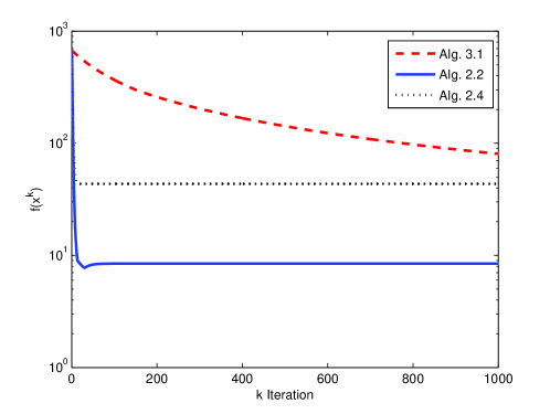
(a) Case 1

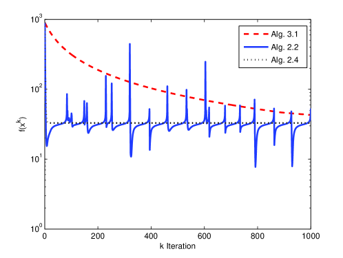
(b) Case 2

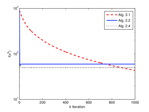
(c) Case 3

Figure 1: Simulation results for a small-scale problem, comparing Algorithms 2.2, 2.4 and 3.1.

The mid-sized problems of Cases 4 and 5 are depicted by Figures 2(a) and 2(b). Figure 2(a) shows that Algorithm 3.1 detects a feasible solution, while both Algorithms 2.2 and 2.4 fail to detect such a solution. The curve of Algorithm 3.1 in Fig. 2(a) stops when it reaches the feasible point detection tolerance, which is 0.1. Once the point is detected, there is no need to further iterate, and the process stops. The curve for Algorithm 2.2 in this figure shows irregular behavior since it searches for a feasible solution without reaching the detection threshold of 0.1 and accumulated numerical errors start to affect it. Figure 2(b) shows a phenomenon similar to the one observed in the small-scale problem: Algorithm 3.1 continues to seek for a feasible solution, while Algorithms 2.2 and 2.4 converge to a steady-state, indicating failure to detect a feasible solution.

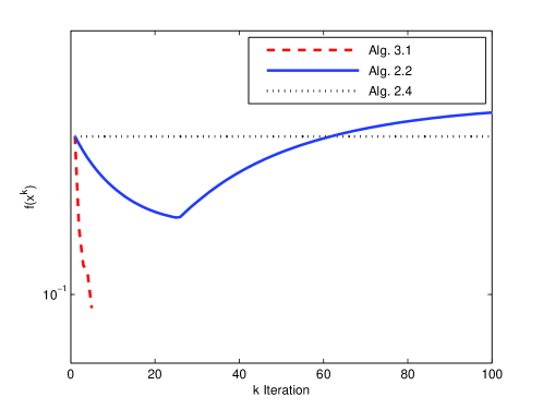
(a) Case 4

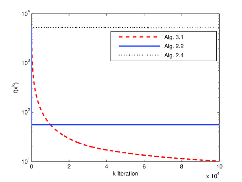
(b) Case 5

Figure 2: Simulation results for a mid-scale problem, comparing Algorithms 2.2, 2.4 and 3.1.

In the experiments, Cases 6–8, Algorithm 3.1 outperforms the other algorithms, arriving very close to finding feasible solutions. It should be observed that the behavior of Algorithm 3.1 observed above is the result of the way in which the relaxation parameters $\lambda_{k}$ are self-regulating their sizes. In Algorithm 3.1 the relaxation parameter $\lambda_{k}$ can be chosen (see Equation (3.6)) to be any number of the form

$$\lambda_{k}=\beta_{k}\frac{\max(0,f(x^{k}))}{M^{2}}+2(1-\beta_{k})\frac{\max(0,f(x^{k}))}{M^{2}}=(2-\beta_{k})\frac{\max(0,f(x^{k}))}{M^{2}},$$ (6.7)

where $\beta_{k}$ runs over the interval $\left[0,1\right].$ Consequently, the size of $\lambda_{k}$ can be very close to zero when $x^{k}$ is close to a feasible solution (no matter how $\beta_{k}$ is chosen in $\left[0,1\right])$. Also, $\lambda_{k}$ may happen to be much larger then $2$ when $x^{k}$ is far from a feasible solution and the number $f(x^{k})$ is large enough (note that $2-\beta_{k}$ stays between 1 and 2). So, Algorithm 3.1 is naturally under- or over- relaxing the computational process according to the relative position of the current iterate $x^{k}$ to the feasibility set of the problem. As our experiments show, in some circumstances, this makes Algorithm 3.1 behave better then the other procedures we compare it with. At the same time, the self-regulation of the relaxation parameters, which is essential in Algorithm 3.1, may happen to reduce the initial speed of convergence of this procedure, that is, Algorithm 3.1 may require more computational steps in order to reach a point $x^{k}$ which is close enough to the feasibility set such that its self-regulatory features to be really advantageous for providing a very precise solution of the given problem (which the other procedures may fail to do since they may became stationary in the vicinity of the feasibility set). Another interesting feature of Algorithm 3.1, which differentiates it from the other algorithms we compare it with, is its essentially non-simultaneous character: Algorithm 3.1 does not necessarily ask for $w_{i}^{k}>0$ for all $i\in\{1,...,m\}.$ The set of positive weights $w_{i}^{k}$ which condition the progress of the algorithm at step $k$ essentially depends on the current iterate $x^{k}$ (see (3.4)) and allows reducing the number of subgradients needed to be computed at each iterative step (in fact, one can content himself with only one $w_{i}^{k}>0$ and, thus, with a single subgradient $\xi_{i}^{k}$). This may be advantageous in cases when computing subgradients is difficult and, therefore, time consuming.

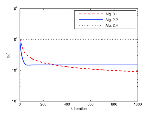
(a) Case 6

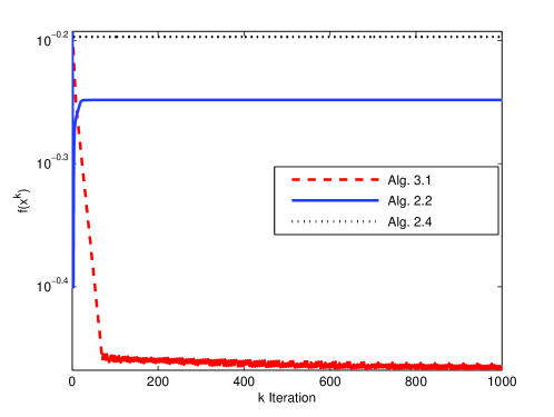
(b) Case 7

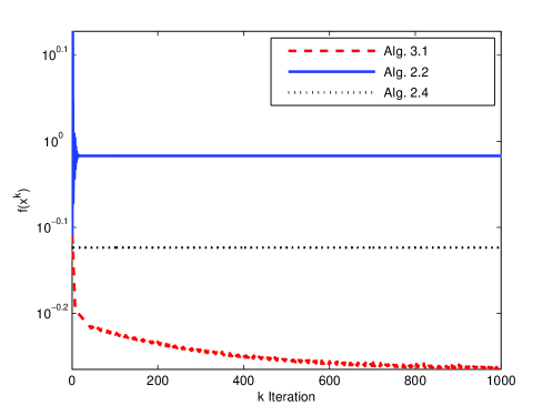
(c) Case 8

Figure 3: Simulation results for small- and mid-scale problems with overrelaxation, comparing Algorithms 2.2, 2.4 and 3.1.

The main observations can be summarized as follows:

1. Algorithm 3.1 exhibits faster initial convergence than the other algorithms in the vicinity of points with very small $f(x^{k})$. When the algorithms reach points with small $f(x^{k})$ values, then Algorithm 3.1 tends to further reduce the value of $f(x^{k})$, while the other algorithms tend to converge onto a constant steady-state value.

2. The problem dimensions in our experiments have little impact on the behavior of the algorithms.

3. All the examined small-scale problems have no feasible solutions. This can be seen from the fact that all three algorithms stabilize around $f(x^{k})=50$.

4. The chaotic oscillations of Algorithm 2.2 in the underrelaxed case is due to the fact that this algorithm has no internal mechanism to self-adapt its progress to the distance between the current iterates and the sets whose intersections are to be found. This phenomenon can hardly happen in Algorithm 3.1 because its relaxation parameters are self-adapting to the size of the current difference between successive iterations. This is an important feature of this algorithm. However, this feature also renders it somewhat slower than the other algorithms.

5. In some cases, Algorithms 2.2 and 2.4 indicate that the problem has no solution. In contrast, Algorithm 3.1 continues to make progress and seems to indicate that the problem has a feasible solution. This phenomenon is again due to the self-adaptation mechanism, and can be interpreted in one of the following ways: (a) The problem indeed has a solution but Algorithms 2.2 and 2.4 are unable to detect it (because they stabilize too fast). Algorithm 3.1 detects a solution provided that it is given enough running time; (b) The problem has no solution and then Algorithm 3.1 will stabilize close to zero, indicating that the problem has no solution, but this may be due to computing (round-off) errors. Thus, a very small perturbation of the functions involved in the problem may render the problem feasible.

7 Conclusions

We have studied here mathematically and experimentally subgradient projections methods for the convex feasibility problem. The behavior of the fully simultaneous subgradient projections method in the inconsistent case is not known. Therefore, we studied and tested two options. One is the use of steering parameters instead of relaxation parameters and the other is a variable relaxation strategy which is self-adapting. Our small-scale and mid-scale experiments are not decisive in all aspects and call for further research. But one general feature of the algorithm with the self-adapting strategical relaxation is its stability (non-oscillatory) behavior and its relentless improvement of the iterations towards a solution in all cases. At this time we have not yet refined enough our experimental setup. For example, by the iteration index $k$ on the horizontal axes of our plots we consider a whole sweep through all sets of the convex feasibility problem, regardless of the algorithm. This is a good first approximation by which to compare the different algorithms. More accurate comparisons should use actual run times. Also, several numerical questions still remain unanswered in this report. These include the effect of various values of the constant $\sigma$ as well as algorithmic behavior for higher iteration indices. In light of the applications mentioned in Section 1, higher dimensional problems must be included. These and other computational questions are currently investigated.

Acknowledgments. We gratefully acknowledge the constructive comments of two anonymous referees which helped us to improve an earlier version of this paper. This work was supported by grant No. 2003275 of the United States-Israel Binational Science Foundation (BSF), by a National Institutes of Health (NIH) grant No. HL70472, by The Technion - University of Haifa Joint Research Fund and by grant No. 522/04 of the Israel Science Foundation (ISF) at the Center for Computational Mathematics and Scientific Computation (CCMSC) in the University of Haifa.

References

- [1] R. Aharoni and Y. Censor, Block-iterative projection methods for parallel computation of solutions to convex feasibility problems, Linear Algebra and Its Applications 120 (1989), 165–175.
- [2] A. Auslender, Optimisation: Méthodes Numériques, Masson, Paris, France, 1976.
- [3] H.H. Bauschke, The approximation of fixed points of compositions of nonexpansive mappings in Hilbert space, Journal of Mathematical Analysis and Applications 202 (1996), 150–159.
- [4] H.H. Bauschke and J.M. Borwein, On projection algorithms for solving convex feasibility problems, SIAM Review 38 (1996), 367–426.
- [5] H.H. Bauschke, J.M. Borwein and A.S. Lewis, The method of cyclic projections for closed convex sets in Hilbert space, Recent developments in optimization theory and nonlinear analysis (Jerusalem 1995), Contemporary Mathematics 204 (1997), 1–38.
- [6] H.H. Bauschke, P.L. Combettes and S.G. Kruk, Extrapolation algorithm for affine-convex feasibility problems, Numerical Algorithms 41 (2006), 239–274.
- [7] M. Benzi, Gianfranco Cimmino’s contributions to numerical mathematics, Atti del Seminario di Analisi Matematica, Dipartimento di Matematica dell’Università di Bologna. Special Volume: Ciclo di Conferenze in Memoria di Gianfranco Cimmino, March-April 2004, Tecnoprint, Bologna, Italy (2005), pp. 87–109. Available at: http://www.mathcs.emory.edu/~benzi/Web_papers/pubs.html
- [8] S. Boyd, L. El Ghaoui, E. Feron, and V. Balakrishnan, Linear Matrix Inequalities in System and Control Theory, Society for Industrial and Applied Mathematics (SIAM), Philadelphia, PA, USA, 1994.
- [9] L.M. Bregman, The method of successive projections for finding a common point of convex sets, Soviet Mathematics Doklady 6 (1965), 688–692.
- [10] D. Butnariu and A.N. Iusem, Totally Convex Functions for Fixed Points Computation and Infinite Dimensional Optimization, Kluwer Academic Publishers, Dordrecht, The Netherlands, 2000.
- [11] D. Butnariu and A. Mehrez, Convergence criteria for generalized gradient methods of solving locally Lipschitz feasibility problems, Computational Optimization and Applications 1 (1992), 307–326.
- [12] D. Butnariu and E. Resmerita, “Averaged subgradient methods for optimization and Nash equilibria computation”, Optimization 51 (2002), 863–888.
- [13] C.L. Byrne, Block-iterative methods for image reconstruction from projections, IEEE Transactions on Image Processing IP-5, pp. 792–794, 1996.
- [14] Y. Censor, Row-action methods for huge and sparse systems and their applications, SIAM Review 23, pp. 444–466, 1981.
- [15] Y. Censor, Mathematical optimization for the inverse problem of intensity modulated radiation therapy, in: J.R. Palta and T.R. Mackie (Editors), Intensity-Modulated Radiation Therapy: The State of The Art, American Association of Physicists in Medicine, Medical Physics Monograph No. 29, Medical Physics Publishing, Madison, Wisconsin, USA, 2003, pp. 25–49.
- [16] Y. Censor, Computational acceleration of projection algorithms for the linear best approximation problem, Linear Algebra and Its Applications 416 (2006), 111–123.
- [17] Y. Censor, M.D. Altschuler and W.D. Powlis, On the use of Cimmino’s simultaneous projections method for computing a solution of the inverse problem in radiation therapy treatment planning, Inverse Problems 4 (1988), 607–623.
- [18] Y. Censor, D. Gordon and R. Gordon, Component averaging: An efficient iterative parallel algorithm for large and sparse unstructured problems, Parallel Computing 27 (2001), 777–808.
- [19] Y. Censor, D. Gordon and R. Gordon, BICAV: A block-iterative, parallel algorithm for sparse systems with pixel-dependent weighting, IEEE Transactions on Medical Imaging 20 (2001), 1050–1060.
- [20] Y. Censor and A. Lent, Cyclic subgradient projections, Mathematical Programming, 24 (1982), 233–235.
- [21] Y. Censor and S.A. Zenios, Parallel Optimization: Theory, Algorithms, and Applications, Oxford University Press, New York, NY, USA, 1997.
- [22] J.W. Chinneck, The constraint consensus method for finding approximately feasible points in nonlinear programs, INFORMS Journal on Computing 16 (2004), 255–265.
- [23] G. Cimmino, Calcolo approssimato per le soluzioni dei sistemi di equazioni lineari, La Ricerca Scientifica XVI Series II, Anno IX, 1 (1938), 326–333.
- [24] F.H. Clarke, Optimization and Nonsmooth Analysis, John Wiley & Sons, New York, NY, USA, 1983.
- [25] P.L. Combettes, The foundations of set-theoretic estimation, Proceedings of the IEEE 81 (1993), 182–208.
- [26] P.L. Combettes, Inconsistent signal feasibility problems: Least-squares solutions in a product space, IEEE Transactions on Signal Processing SP-42 (1994), 2955–2966.
- [27] P.L. Combettes, The convex feasibility problem in image recovery, Advances in Imaging and Electron Physics 95 (1996), 155–270.
- [28] P.L. Combettes, Convex set theoretic image recovery by extrapolated iterations of parallel subgradient projections, IEEE Transactions on Image Processing 6 (1997), 493–506.
- [29] G. Crombez, Non-monotoneous parallel iteration for solving convex feasibility problems, Kybernetika 39 (2003), 547–560.
- [30] G. Crombez, A sequential iteration algorithm with non-monotoneous behaviour in the method of projections onto convex sets, Czechoslovak Mathematical Journal 56 (2006), 491–506.
- [31] F. Deutsch, Best Approximation in Inner Product Spaces, Springer-Verlag, New York, NY, USA, 2001.
- [32] L.T. Dos Santos, A parallel subgradient method for the convex feasibility problem, Journal of Computational and Applied Mathematics 18 (1987), 307–320.
- [33] I.I. Eremin, Fejér mappings and convex programming, Siberian Mathematical Journal 10 (1969), 762–772.
- [34] L. Gubin, B. Polyak and E. Raik, The method of projections for finding the common point of convex sets, USSR Computational Mathematics and Mathematical Physics 7 (1967), 1–24.
- [35] G.T. Herman, Image Reconstruction From Projections: The Fundamentals of Computerized Tomography, Academic Press, New York, NY, USA, 1980.
- [36] G.T. Herman and L.B. Meyer, Algebraic reconstruction techniques can be made computationally efficient, IEEE Transactions on Medical Imaging 12 (1993), 600–609.
- [37] A.N. Iusem and A.R. De Pierro, Convergence results for an accelerated nonlinear Cimmino algorithm, Numerische Mathematik 49 (1986), 367–378.
- [38] K.C. Kiwiel, The efficiency of subgradient projection methods for convex optimization I: General level methods, SIAM Journal on Control and Optimization 34 (1996), 660–676.
- [39] K.C. Kiwiel, The efficiency of subgradient projection methods for convex optimization II: Implementations and extensions, SIAM Journal on Control and Optimization 34 (1996), 677–697.
- [40] K.C. Kiwiel and B. Lopuch, Surrogate projection methods for finding fixed points of firmly nonexpansive mappings, SIAM Journal on Optimization 7 (1997), 1084–1102.
- [41] A.N. Iusem and L. Moledo, A finitely convergent method of simultaneous subgradient projections for the convex feasibility problem, Computational and Applied Mathematics 5 (1986), 169–184.
- [42] L.D. Marks, W. Sinkler and E. Landree, A feasible set approach to the crystallographic phase problem, Acta Crystallographica A55 (1999), 601–612.
- [43] M. Aslam Noor, Some developments in general variational inequalities, Applied Mathematics and Computation 152 (2004), 197–277.
- [44] D. Pascali and S. Sburlan, Nonlinear Mappings of Monotone Type, Sijthoff & Noordhoff International Publishers, Alphen aan den Rijn, The Netherlands, 1978.
- [45] G. Pierra, Decomposition through formalization in a product space, Mathematical Programming 28 (1984), 96–115.
- [46] R.R. Phelps, Convex Functions, Monotone Operators and Differentiability, second edition, Springer-Verlag, Berlin, Germany 1993.
- [47] H. Stark and Y. Yang, Vector Space Projections: A Numerical Approach to Signal and Image Processing, Neural Nets, and Optics, John Wiley & Sons, New York, NY, USA, 1998.
- [48] I. Yamada, Hybrid steepest descent method for variational inequality problem over the fixed point set of certain quasi-nonexpansive mappings, Numerical Functional Analysis and Optimization 25 (2004), 619–655.
- [49] D.C. Youla, Mathematical theory of image restoration by the method of convex projections, in: H. Stark (Editor), Image Recovery: Theory and Applications, Academic Press, Orlando, Florida, USA, 1987, pp. 29–77.