Overlapping Community Detection in
Bipartite Networks

Abstract

Recent researches have discovered that rich interactions among entities in nature and society bring about complex networks with community structures. Although the investigation of the community structures has promoted the development of many successful algorithms, most of them only find separated communities, while for the vast majority of real-world networks, communities actually overlap to some extent. Moreover, the vertices of networks can often belong to different domains as well. Therefore, in this paper, we propose a novel algorithm BiTector (Bi-community Detector) to efficiently mine overlapping communities in large-scale sparse bipartite networks. It only depends on the network topology, and does not require any priori knowledge about the number or the original partition of the network. We apply the algorithm to real-world data from different domains, showing that BiTector can successfully identifies the overlapping community structures of the bipartite networks.

1 Introduction

In recent years, people have found that both of the physical systems in nature and the engineered artifacts in human society can be modeled as complex networks[1][2], such as the internet, the World Wide Web, social networks, citation networks and etc. Although these systems come from very different domains, they all have the community structure [3][4] in common, that is, they have vertices in a group structure that vertices within the groups have higher density of edges while vertices among groups have lower density of edges.

The existence of the community structures has important practical significance. For example, the communities in World Wide Web correspond to topics of interest. In social networks, individuals belong to the same community are probable to have properties in common. Nowadays, community information is considered to be used for improving the search engine to provide better personalized results. Moreover, the information diffusion and spreading mechanism in a network can be affected and determined by the community structures. Hence, identifying the communities is a fundamental step not only for discovering what makes entities come together, but also for understanding the overall structural and functional properties of the whole network. As a result, a wide range of successful algorithms[5] have been proposed to discover the community structures. These methods assume that communities are separated, placing each vertex in only one community. They do not take into account the possible overlappings[6] among communities in the real-world scenarios, such as that each of us may participate in many social cycles according to our various hobbies.

Moreover, the specific types of the vertices may not belong to the same domain as well, bringing about a bipartite network structure. For example, in the scientific collaboration network[7], two different types of nodes represent the authors and papers respectively; in the movie-actor network[8], each actor is connected to the films where he or she has starred; in the collaborative recommendation network[9], the edges link each customer to the corresponding rated or tagged pages, pictures, videos and other products. In addition, many biological networks are naturally bipartite, such as the protein interaction network from yeast[10], where the two types of nodes are bait proteins and prey proteins, and the human disease network of diseases and their pathogenicity genes[11].

Traditionally, the studies of the bipartite networks usually depend on the one-mode projection of the original network into two unipartite networks. More specifically, given a bipartite network $\mathcal{G}_{(U,I)}$, where $U$ and $I$ are the sets of the two different types of nodes, the one-mode projection converts $\mathcal{G}_{(U,I)}$ into $\mathcal{G}_{U}$ and $\mathcal{G}_{I}$ respectively. The adjacency matrices of $\mathcal{G}_{U}$ and $\mathcal{G}_{I}$ are built such that

$$E_{ij}(\mathcal{G}_{U})=\left\{\begin{array}[]{l@{\quad}l}1&\textrm{if vertex }i\textrm{ and }j\textrm{ have a common neighbor }i_{k}\in I\textrm{ in }\mathcal{G}_{(U,I)}\\ 0&\textrm{otherwise}\\ \end{array}\right.$$

and

$$E_{ij}(\mathcal{G}_{I})=\left\{\begin{array}[]{l@{\quad}l}1&\textrm{if vertex }i\textrm{ and }j\textrm{ have a common neighbor }u_{k}\in U\textrm{ in }\mathcal{G}_{(U,I)}\\ 0&\textrm{otherwise}\\ \end{array}\right.$$

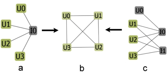
Figure 1: One-mode projection

Thus, many existing community detection algorithms can be applied to $\mathcal{G}_{U}$ and $\mathcal{G}_{I}$ accordingly. Although this projection approach is simple and intuitive, it may suffer from the loss of information problem. In general, the real world bipartite network $\mathcal{G}_{(U,I)}$ is a large sparse graph. However, the generated graph $\mathcal{G}_{U}$ and $\mathcal{G}_{I}$ may become very dense as a result of the projection. In Fig.1a, U0, U1, U2, and U3 have a common neighbor I0, so they form a 4-clique (complete graph) in Fig.1b by projection. Similarly, we can also obtain the same 4-clique from Fig.1c. However, it is easy to see that in Fig.1c, there exists a more closer relationship among U1, U2, and U3 for that they all have connections with both I0 and I1. Yet, in Fig.1b, the four nodes are indistinguishably equivalent with each other. This problem is very common in real life networks. For example, in collaborative recommendation network, a very popular film can be rated by hundreds of users just like the scenario shown in Fig.1a. If we project the original graph into the network consisting of all the users, it will contain a huge clique formed by these hundreds of users. As a result, due to the existence of many superfluous edges generated by the one-mode projection, the truly meaningful information may be overwhelmed by the high link density.

Consequently, the main contributions of this paper concentrate on mining overlapping communities directly on the bipartite networks. We would like to answer the questions like what groups of people are interested in what types of products, or what cycles of scientists prefer to collaborate in what kind of research areas. The rest of the paper is thus organized as follows: in section 2, we mainly review some related work. Section 3 describes the overlapping community detection algorithm BiTector in details. Experimental results and analysis are presented in section 4; and we conclude the paper in section 5.

2 Related Work

One of the classic approaches for detecting community structures in unipartite networks is the GN algorithm[12] that introduces a network modularity metric and optimizes it globally to find the non-overlapping communities. Guimerà[13] et al. generalizes this modularity metric to the bipartite networks. They first differentiate the two parts of the network as the actors and teams, and then formulate the bipartite modularity from the groups of actors that are closely interconnected based on joint participation in many teams. Given vertex $v_{i}$ and $v_{j}$, the bipartite modularity is defined as the cumulative deviation of the number of the actual teams where $v_{i}$ and $v_{j}$ have been involved from the random expectation. Similarly, $Barber$[14] defines the bipartite modularity matrix B as an extension of Newman’s recent work[15]. Some key properties of the eigenspectrum of B are identified and used to specialize Newman’s matrix-based algorithms to bipartite networks.

In parallel, Lehmann[16] et al. extend the $k$-clique community definition from Palla’s work[6]. They define a $K_{a,b}$ biclique community as a union of all $K_{a,b}$ bicliques that can be reached from each other through a series of adjacent $K_{a,b}$ bicliques, where $a$ and $b$ are the vertices’ number belonging to the two different vertex sets respectively. Just like Palla’s work, two $K_{a,b}$ bicliques are to be adjacent if their overlap is at least a $K_{a-1,b-1}$ biclique.

To sum up, the modularity-based algorithms, like $GN$ with $O(m^{3})$ time complexity ($m$ is the number of edges), are designed to find the non-overlapping communities and often have the efficiency problem which makes them unsuitable to the large-scale networks in practical scenarios. Moreover, the modularity optimization strategy may introduce a resolution limit[17] as well. For Lehmann’s algorithm, since it extends from Palla’s work, the required user input value $k$, the lower and upper limit value of the community size, often put a significant impact on the discovered communities, and are uneasy to be determined before the algorithm can run. In addition, vertices that are not included in any $K_{a,b}$ bicliques will be ignored, so the set of all the detected communities usually can not cover all the vertices of the original graph.

Therefore, to overcome these shortages, we propose BiTector by a local optimization strategy, which does not suffer from the resolution problem, and does not require any priori knowledge about the community’s number or other related thresholds to assess the community structure. As of this writing, BiTector is the first method that can handle bipartite networks consisting of millions of nodes and edges.

3 BiClique-based Overlapping Community Detection Algorithm

Instead of dividing a network into its most loosely connected parts, BiTector identifies the communities based on the most densely connected parts, namely, the bicliques. We treat each group of highly overlapping maximal bicliques as the clustering cores. Surrounding each core, we build up the communities in an gradually expanding way according to certain metrics until each vertex in the network belongs to at least one community.

3.1 Notations and Definitions

In this paper, we consider simple and connected graphs only, i.e., the graphs without self-loops or multi-edges. Given graph $\mathcal{G}_{(U,I)}$, where $U$ and $I$ or $U_{\mathcal{G}}$ and $V_{\mathcal{G}}$ are the sets of the two different types of nodes, $V(\mathcal{G}_{(U,I)})=U_{\mathcal{G}}\cup I_{\mathcal{G}}$ and $E(\mathcal{G}_{(U,I)})$ denote the sets of all its vertices and edges respectively.

Definition 1

Given sub-bigraph $S_{(U,I)},U_{S}\subseteq U_{\mathcal{G}},I_{S}\subseteq I_{\mathcal{G}}$, if $\forall u_{i}\in U_{S},v_{j}\in I_{S}$, $\exists e_{(u_{i},v_{j})}\in E(S_{(U,I)})$, then $S_{(U,I)}$ is a biclique. If there is no any other biclique $S^{\prime}_{(U,I)}$, such that $U_{S}\subset U_{S^{\prime}}$ and $I_{S}\subset I_{S^{\prime}}$, $S_{(U,I)}$ is called the maximal bicliques.

Definition 2

For a given vertex $v$, $N(v)=\{u|(v,u)\in E(G)\}$, we call $N(v)$ is the neighbor set of $v$. For sub-bigraph $S_{(U,I)}$, $N(U_{S})=\bigcup N(u_{i})-I_{S},u_{i}\in U_{S}$, and $N(I_{S})=\bigcup N(v_{j})-U_{S},v_{j}\in I_{S}$, $N(U_{S})\cup N(I_{S})$ is called the neighbor set of $S_{(U,I)}$.

Definition 3

$\mathcal{M}(\mathcal{G}_{(U,I)})$ denotes the set of all maximal bicliques $B_{(U,I)}$ $(|U_{B}|\geq 2,|I_{B}|\geq 2)$ in $\mathcal{G}_{(U,I)}$. Given vertex $v_{i}\in V(\mathcal{G}_{(U,I)})$, $\mathcal{B}(v_{i})\subseteq\mathcal{M}(\mathcal{G}_{(U,I)})$ is the set of all maximal bicliques that contain $v_{i}$. The set of all $\mathcal{B}(v_{i})$ is denoted as $\mathcal{B}$. For any pair of sub-bigraph $\mathcal{G}_{i}$ and $\mathcal{G}_{j}$, a Closeness Function $isClose(\mathcal{G}_{i},\mathcal{G}_{j})$ is defined and implemented in the next section to identify whether they could be merged together by quantifying how ”close” they actually can be. Given any two maximal bicliques $B_{m},B_{n}\in\mathcal{B}(v_{i}),|U_{B_{m}}|>|U_{B_{n}}|$, $\mathcal{G}_{m}$ and $\mathcal{G}_{n}$ are the bi-subgraphs induced on $B_{m}$ and $B_{n}$ respectively. If $isClose(\mathcal{G}_{m},\mathcal{G}_{n})$ returns true, we say $B_{n}$ is contained by $B_{m}$, denoted by $B_{n}<B_{m}$. If $B_{m}$ is not contained by any other maximal bicliques in $\mathcal{B}(v_{i})$, $B_{m}$ is called the $\mathbf{core}$ and the set of all cores is denoted by $\mathcal{C}$.

Definition 4

Let $S_{0}$,$S_{1}$,…,$S_{n-1}$ be the sub-bigraph of $\mathcal{G}_{(U,I)}$ such that $V(S_{0})\cup$,…,
$V(S_{n-1})=V(\mathcal{G}_{(U,I)})$. For any pair of $S_{i}$ and $S_{j}$, if $|E(S_{i})|>|E_{between}(S_{i},S_{j})|$, $S_{i}$ is defined as the community of $\mathcal{G}_{(U,I)}$.

3.2 Algorithm

BiTector first enumerates all maximal bicliques in $\mathcal{G}_{(U,I)}$. Because a maximal biclique is a complete sub-bigraph, it is thus the densest community structure which can represent the closest relationship between the two types of vertices in the given network. Given two sub-bigraphs $\mathcal{G}_{i}$ and $\mathcal{G}_{j}$, the basic idea of the closeness function $isClose(\mathcal{G}_{i},\mathcal{G}_{j})$ depends on the link pattern between $\mathcal{G}_{i}$ and $\mathcal{G}_{j}$ to quantify the influence that they put on each other. We use $\Delta_{ij}$ to denote the common vertices between $U_{\mathcal{G}_{i}}$ and $U_{\mathcal{G}_{j}}$, and $\Gamma_{ij}$ to denote the common vertices between $I_{\mathcal{G}_{i}}$ and $I_{\mathcal{G}_{j}}$ accordingly. The left sub-bigraph of $\mathcal{G}_{i}$ is then defined as $\mathcal{L}_{i}$ with $U_{\mathcal{L}_{i}}=U_{\mathcal{G}_{i}}-\Delta_{ij}$ and $I_{\mathcal{L}_{i}}=I_{\mathcal{G}_{i}}-\Gamma_{ij}$. Similarly, the left sub-bigraph of $\mathcal{G}_{j}$ is denoted as $\mathcal{L}_{j}$ with $U_{\mathcal{L}_{j}}=U_{\mathcal{G}_{j}}-\Delta_{ij}$ and $I_{\mathcal{L}_{j}}=I_{\mathcal{G}_{j}}-\Gamma_{ij}$. We define the sub-bigraphs induced on $U_{\mathcal{L}_{i}}\cup I_{\mathcal{L}_{j}}$, and $U_{\mathcal{L}_{j}}\cup I_{\mathcal{L}_{i}}$ are $\mathcal{G}_{(U_{\mathcal{L}_{i}},I_{\mathcal{L}_{j}})}$ and $\mathcal{G}_{(U_{\mathcal{L}_{j}},I_{\mathcal{L}_{i}})}$ accordingly. Here the influence that $\mathcal{G}_{i}$ puts on $\mathcal{G}_{j}$ is defined based on $U_{\mathcal{G}_{i}}$. It is equivalent if we start from $I_{\mathcal{G}_{i}}$.

$$inf_{ij}=|E(\mathcal{G}_{(U_{\mathcal{L}_{i}},I_{\mathcal{L}_{j}})})|+|E(\mathcal{G}_{(U_{\mathcal{L}_{j}},I_{\mathcal{L}_{i}})})|-|E(\mathcal{L}_{j})|$$

It is apparent that for $\mathcal{G}_{i}$ and $\mathcal{G}_{j}$, $inf_{ij}$ actually reflects the number of edges between them minus that of $\mathcal{G}_{j}$’s inner edges. If both $inf_{ij}\geq 0$ and $inf_{ji}\geq 0$, then $\mathcal{G}_{i}$ and $\mathcal{G}_{j}$ should be merged together as a single graph; otherwise, they will be separated apart. The implementation of $isClose(\mathcal{G}_{i},\mathcal{G}_{j})$ is formulated in Algorithm 1.

To make things more concrete, an illustrated example is given on the network shown in Fig.2. There are two sub-bigraphs: $\mathcal{G}_{0}$ cycled by red dashed-line, and $\mathcal{G}_{1}$ cycled by green dashed-line. $U_{\mathcal{G}_{0}}=\{U_{0},U_{1},U_{2}\}$. $I_{\mathcal{G}_{0}}=\{I_{0},I_{1},I_{2}\}$. $U_{\mathcal{G}_{1}}=\{U_{3},U_{4}\}$. $I_{\mathcal{G}_{1}}=\{I_{3},I_{4},I_{5}\}$. $inf_{01}=2+2-6=-2<0$, and $inf_{10}=2+2-8=-4<0$, so $\mathcal{G}_{0}$ and $\mathcal{G}_{1}$ should not be merged together.

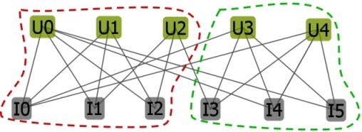
Figure 2: Example of Core Formation

Starting from $\mathcal{M}(\mathcal{G}_{(U,I)})$, we first find $\mathcal{B}(u_{i})\in\mathcal{B}$ for every vertex $u_{i}\in\mathcal{G}_{(U,I)}$. Because every maximal biclique in $\mathcal{B}(u_{i})$ corresponds to one group of vertices in $U_{\mathcal{G}}$ which together with $u_{i}$ are closely interconnected based on the jointly connections with certain cluster of vertices in $I_{\mathcal{G}}$, $\mathcal{B}(u_{i})$ covers all the densest communities where $u_{i}$ has participated. $\forall u_{i},u_{j}\in U_{\mathcal{G}}$, $\mathcal{G}_{i}$ and $\mathcal{G}_{j}$ represent the sub-bigraphs induced on $\mathcal{B}(u_{i})$ and $\mathcal{B}(u_{j})$. If $isClose(\mathcal{G}_{i},\mathcal{G}_{j})$ returns true, which means all or most of $u_{j}$’s relationships are covered by those of $u_{i}$, $u_{j}$ should thus stay in the same community with $u_{i}$. We rearrange the elements of $\mathcal{B}$ according to the descending order of $|\mathcal{B}(u_{i})|$. Let $|\mathcal{B}(u_{k})|$ be the element of $\mathcal{B}$ whose size is the largest. We put $|\mathcal{B}(u_{k})|$ to set $\mathcal{H}$ and removed it from $\mathcal{B}$. All the other elements contained by $|\mathcal{B}(u_{k})|$ are also removed from $\mathcal{B}$. Again, we pick the next largest element of $\mathcal{B}$, put it to $\mathcal{H}$, removed it as well as those elements it contains from $\mathcal{B}$. The process is continued until $\mathcal{B}$ is empty, so set $\mathcal{H}$ stores the elements being independent of each other.

Algorithm 1 $isClose(\mathcal{G}_{i},\mathcal{G}_{j})$

1:  { $\mathcal{G}_{L}\Leftarrow\mathcal{G}_{i}$ or $\mathcal{G}_{j}$ with the larger set of $U$, $\mathcal{G}_{S}\Leftarrow\mathcal{G}_{i}$ or $\mathcal{G}_{j}$ with the smaller set of $U$}

2:  {$\Delta=U_{\mathcal{G}_{L}}\cap U_{\mathcal{G}_{S}}$, $\Gamma=I_{\mathcal{G}_{L}}\cap I_{\mathcal{G}_{S}}$}

3:  if $U(\mathcal{G}_{S})\subseteq U(\mathcal{G}_{L})$ or $I(\mathcal{G}_{S})\subseteq I(\mathcal{G}_{L})$) or $(I(\mathcal{G}_{L})\subseteq I(\mathcal{G}_{S}))$ then

4:     return true

5:  else

6:     $C_{L}=|E(\mathcal{G}_{(\Delta,\Gamma)})|-|E(\mathcal{L}_{L})|$

7:     $C_{S}=|E(\mathcal{G}_{(\Delta,\Gamma)})|-|E(\mathcal{L}_{S})|$

8:     if $(C_{L}\geq 0)$ or $(C_{S}\geq 0)$ or ($inf_{LS}\cdot inf_{SL}\geq 0)$ then

9:        return true

10:     end if

11:  end if

12:  return false

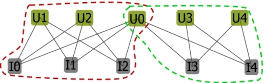
Figure 3: Example of Core Formation

In general, the distribution of the vertex degree in bipartite networks conforms to a power-law. It is common that a few vertices in $U_{\mathcal{G}}$ have connections with nearly all vertices in $I_{\mathcal{G}}$. As a result, these vertices can appear in lots of maximal bicliques repeatedly. For example, in Fig.3, we can see that $\mathcal{B}(U0)=\{\{U0,U1,U2,I0,I1,I2\},\{U0,U3,U4,I3,I4\}\}$, and $U0$ has connections with all the vertices from $I0$ to $I4$. However, it is obvious that $\{U0,U1,U2,I0,I1,I2\}$ and $\{U0,U3,U4,I3,I4\}$ are two different communities with a overlapping vertex $U0$. Consequently, to address this problem, given $u_{i}$ and $\mathcal{B}(u_{i})$, we need to further refine $\mathcal{B}(u_{i})$ into several sub-bigraphs representing different communities that $u_{i}$ has taken part in simultaneously. Therefore, for each element $H_{k}\in\mathcal{H}$, every maximal biclique $B_{m}\in H_{k}$ is sorted by the descending order of $U_{B_{m}}$. Given $B_{m},B_{n}$ with $|U_{B_{m}}|\geq|U_{B_{n}}|$, if $isClose(\mathcal{G}_{m},\mathcal{G}_{n})$ returns true, $B_{n}$ is thus contained by $B_{m}$. If $B_{m}$ is not contained by any other elements in $H_{k}$, $B_{m}$ is regarded as the core, and will be put in set $\mathcal{C}$. This process is continued until every element in $\mathcal{H}$ has been refined. The whole procedure is described in algorithm 2.

Algorithm 2 $CoreFormation(\mathcal{M}(\mathcal{G}_{(U,I)}))$

1:  $\mathcal{C}\Leftarrow\emptyset$, $\mathcal{H}\Leftarrow\emptyset$, $contained\Leftarrow\emptyset$

2:  Get $\mathcal{B}$ from $\mathcal{M}(\mathcal{G}_{(U,I)})$ and sort $\mathcal{B}(u_{i})\in\mathcal{B}$ by the descending order of $|\mathcal{B}(u_{i})|$

3:  for $\forall\mathcal{B}(u_{i})\in\mathcal{B}$ do

4:     if $\mathcal{B}(u_{i})\not\in contained$ then

5:        $contained\Leftarrow\mathcal{B}(u_{j})$, if $isClose(\mathcal{G}_{i},\mathcal{G}_{j})$ returns true

6:        add $\mathcal{B}(u_{i})$ to $\mathcal{H}$

7:     end if

8:  end for

9:  for $\forall H_{k}\in\mathcal{H}$ do

10:     $contained\Leftarrow\emptyset$

11:     for $\forall B_{m}\in H_{k}$ do

12:        if $B_{m}\not\in contained$ then

13:           $contained\Leftarrow B_{n}$, $B_{n}<B_{m}$

14:           add $B_{m}$ to $\mathcal{C}$

15:        end if

16:     end for

17:  end for

18:  return $\mathcal{C}$

3.2.1 Clustering

Once all the cores have been detected, we carry out a clustering process to associate the left vertices to their ”closest” cores. For each sub-bigraph $\mathcal{G}_{i}$ induced on $C_{i}\in\mathcal{C}$, we gradually expand $\mathcal{G}_{i}$ by adding the vertices in set $N(U_{\mathcal{G}_{i}})\cup N(I_{\mathcal{G}_{i}})$. Given vertex $\forall v_{i}\in V(\mathcal{G}_{(U,I)})$ and $\forall C_{j}\in\mathcal{C}$, the distance between $v_{i}$ and $\mathcal{G}_{j}$ is defined as follows:

$$\mathcal{D}(v_{i},\mathcal{G}_{j})=\left\{\begin{aligned} \frac{|N(v_{i})\cap I_{\mathcal{G}_{j}}|}{|N(v_{i})\cup I_{\mathcal{G}_{j}}|}&,v_{i}\in U_{\mathcal{G}}\\ \frac{|N(v_{i})\cap U_{\mathcal{G}_{j}}|}{|N(v_{i})\cup U_{\mathcal{G}_{j}}|}&,v_{i}\in I_{\mathcal{G}}\\ \end{aligned}\right.$$

As a consequence, $v_{i}$ is assigned to the cores with the maximum distance value. Since that any vertex might have the same maximum distance value with more than one core, $v_{i}$ can thus be assigned to multiple cores simultaneously.

Since that for vertex $v_{i}$, it actually does not have connections with all the cores in $\mathcal{C}$. Therefore, we adopt a coloring strategy to reduce the computation cost. First, the vertices covered by all cores in $\mathcal{C}$ are colored as old. We use set $U_{\mathcal{C}}\subseteq U_{\mathcal{G}}$ and $I_{\mathcal{C}}\subseteq I_{\mathcal{G}}$ to store the two types of vertices covered by $\mathcal{C}$. Next, every new vertex in $N(U_{\mathcal{C}})$ and $N(I_{\mathcal{C}})$ is assigned to its closest cores, and colored as old. As a result, every core is now expanded. Again, starting from $N(U_{\mathcal{C}})$ and $N(I_{\mathcal{C}})$, all new vertices that have not been colored in $N(N(U_{\mathcal{C}}))$ and $N(N(I_{\mathcal{C}}))$ are going to be assigned and colored. The clustering continues until all the vertices of the network are colored as old.

Algorithm 3 $Clustering(\mathcal{C})$

1:  for $C_{i}\in\mathcal{C}$ do

2:     $\forall v_{k}\in V(\mathcal{G}_{C_{i}})$ is marked as old

3:  end for

4:  $U_{Exp}\Leftarrow N(I_{\mathcal{C}})$, $I_{Exp}\Leftarrow N(U_{\mathcal{C}})$

5:  while not all vertices in $V(\mathcal{G}_{(U,I)})$ are colored do

6:     for $\forall v_{i}\in U_{Exp}\cup I_{Exp}$ do

7:        if $v_{i}$ is not colored then

8:           assign $v_{i}$ to its closest core, and color $v_{i}$ as old

9:        end if

10:     end for

11:     $U^{\prime}_{Exp}\Leftarrow\emptyset$, $I^{\prime}_{Exp}\Leftarrow\emptyset$

12:     add $v_{j}$ to $U^{\prime}_{Exp}$, if $\forall v_{j}\in N(I_{Exp})$ and $v_{j}$ is not colored

13:     add $v_{k}$ to $I^{\prime}_{Exp}$, if $\forall v_{k}\in N(U_{Exp})$ and $v_{k}$ is not colored

14:     $U_{Exp}\Leftarrow U^{\prime}_{Exp}$, $I_{Exp}\Leftarrow I^{\prime}_{Exp}$

15:  end while

16:  sort $Core$ according to descending order of $|U_{\mathcal{G}_{C_{i}}}|,C_{i}\in Core$

17:  for $C_{i}\in\mathcal{C}$ do

18:     if $C_{i}$ is not merged then

19:        $C_{j}$ is merged to $C_{i}$, if $isClose(\mathcal{G}_{i},\mathcal{G}_{j})$ returns $true$.

20:     end if

21:  end for

In the end, let $\mathcal{C}^{\prime}$ denote the set of every expanded core. We use the same process as the Core Formation to compare the closeness between $C^{\prime}_{i}$ and $C^{\prime}_{j}\in\mathcal{C}^{\prime}$. If $isClose(\mathcal{G}^{\prime}_{i},\mathcal{G}^{\prime}_{j})$ returns $true$, $C^{\prime}_{i}$ and $C^{\prime}_{j}$ is merged together. The whole process is presented in algorithm 3.

3.3 Complexity

Like the classic maximal clique problem in unipartite network, the enumeration of all maximal bicliques is a NP problem as well. However, for most real world bipartite networks, they are often large sparse graphs$(N=|V(\mathcal{G})|,M=|E(\mathcal{G})|,N\approx M)$, and there exist modern algorithms that are very efficient on sparse graphs. Because the enumeration of maximal bicliques is equivalent to the Closed Item Set problem, we use the LCM (Linear time Closed itemset Miner)[18] to mine all the maximal bicliques. On sparse graphs, the computational complexity of LCM is almost proportional to $O(M)$. The calculation of set $\mathcal{H}$ costs $O(N)$. Let $S_{C}$ be the maximum size of $\mathcal{B}(u_{i})\in\mathcal{B}$. It costs $O(|\mathcal{H}|\times S_{C})$ to calculate the core set $\mathcal{C}$. In the end, the clustering process costs $O(N\times|\mathcal{C}|)$. Because on sparse bipartite networks $|\mathcal{M}(\mathcal{G}_{(U,I)})|\approx N\approx M$, $|\mathcal{H}|\ll N$, $S_{C}<|\mathcal{C}|\ll|\mathcal{M}(\mathcal{G}_{(U,I)})|$, the total complexity of $BiTector$ is therefore $O(M^{2})$.

4 Experimental Results

In this section, we will present the experimental results and analysis on several real, large bipartite networks from different domains. All experiments are done on a single PC (3.0GHz processor with 2Gbytes of main memory on Linux AS3 OS). The execution time of BiTector includes both of the biclique finding time and the community detection time. The experimental results are shown in Table 1.

Table 1: Experimental Results

Graph	Vertices $|V|$	Edges $|E|$	Time(s)
DAVIS SOUTHERN CLUB WOMEN[19]	32	93	0.5
NATION-SPORT NETWORK OF OLYMPIC GAMES[20]	515	208	1
CUSTOMER-PRODUCT NETWORK[21]	2008	3258	2
PROTEIN INTERACTION NETWORK OF YEAST[22]	3,740	4,480	2
AUTHOR-PAPER NETWORK OF arXiv[23]	20,454	24,154	6
MOVIE-RATING NETWORK OF NETFLIX[24]	75,179	100,000	92
BOOK-RATING NETWORK[25]	263,804	433,695	4,028
IMDB NETWORK[22]	289,435	637,035	4,312

4.0.1 DAVIS SOUTHERN CLUB WOMEN.

The Southern women data set describes the participation of 18 women in 14 social events. The women and social events constitute a bipartite network; an edge exists between a woman and a social event if the woman was in attendance at the event. This data set have been much studied by Davis as part of an extensive study of class and race in the Deep South. $BiTector$ finds 4 overlapping communities shown in Fig.4.

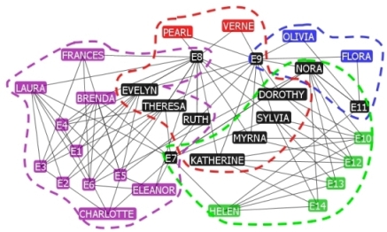
Figure 4: SOUTHERN CLUB WOMEN

Each community is circled by one colored dashed-line, and the overlapping vertices are colored by Black. It is apparent that $E8$ and $E9$ are two very famous clubs attracting 9 women to join. Similarly, Barber’s algorithm also gets 4 separated communities, while Guimerà’s method finds two coarse ones.

4.0.2 CUSTOMER-PRODUCT NETWORK

is derived from the purchase data of Gazelle.com, a legwear and legcare web retailer that closed their online store on 8/18/2000. An edge connects a customer to the products he or she has ordered.

4.0.3 PROTEIN INTERACTION NETWORK OF YEAST

contains two types of proteins. One represents the bait proteins and the other represents the prey proteins. An edge links a prey protein to a bait protein if the prey protein binds to the bait one.

4.0.4 AUTHOR-PAPER NETWORK OF arXiv

presents the relationships among authors and papers. An edge links an author to a paper if this author has published the paper before. Each discovered community in this network can intuitively links certain experts to their research areas that are reflected by the published papers on which they have once collaborated. Fig.5 describes one community where Prof. M.E.J. Newman has been involved. Newman has proposed the classic $GN$ algorithm[12] for community detection in unipartite networks, and the community detected by $BiTector$ in Fig.5 can directly finds one of the circles where he has been often involved in the physics society.

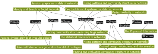
Figure 5: Experts with Research Areas

4.0.5 MOVIE-RATING NETWORK OF NETFLIX

is composed of users and their rated movies. Netflix provides an evaluation mechanism that enables users to rate movies from score 0 to score 10 to express their preferences. There exists an edge between a user and a movie if this user has rated the movie. In our experiment, we build the network from Netflix’s rating data in 2006.

4.0.6 BOOK-RATING NETWORK

is built from the Book-Crossing community. In our experiment, there exists en edge between a user and a book if this user has given a non-zero rating score to the book.

4.0.7 IMDB NETWORK

is composed of actors and movies. A link connects an actor or actress to a movie he or she has once starred.

4.0.8

In the experiments, except for the DAVIS SOUTHERN CLUB WOMEN, both Barber’s and Guimerà’s algorithms are not suitable to run on the other datasets within the acceptable time. For Lehmann’s algorithm, since the discovered communities depend on the user input value $k$, and the required lower bound and upper bound of the community size, we do not include the correspondent results here. We further evaluate the homogeneity of $BiTector$’s discovered communities by comparing them with their counterparts in the random bipartite networks.

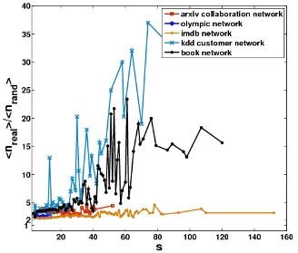
Figure 6: Communities’ Homogeneity

For any discovered community $C_{(U,I)}$, we first randomly choose $|U_{C}|$ vertices from $U_{\mathcal{G}}$ into set $U_{R}$. Then from the union neighbor set of the chosen vertices, we further randomly choose $|I_{C}|$ vertices into set $I_{R}$. As a consequence, we obtain a randomly generated community $R_{(U,I)}$ having the same size with $C_{(U,I)}$. In Fig.6, each symbol corresponds to the average number of the inner edges for a given community size, $n_{<real>}$, divided by the same quantity found in random sets, $n_{<rand>}$. We can see that the $n_{<real>}/n_{<rand>}$ ratio is significantly larger than 1, indicating that the communities discovered by BiTector tend to contain closely interrelated entities, a homogeneity that supports the validity and effectiveness of the discovered communities.

4.0.9 NATION-SPORT NETWORK OF OLYMPIC GAMES

. Besides the bipartite networks we just discussed above, $BiTector$ is further challenged on the networks of Olympic Games in Summer from 1896 to 2004. In each year, we build the network according the relationships between nations and the correspondent sports. An edge links a nation and a specific sport if the nation has won medals in that sport. There are totally 25 networks being built from 1896 to 2004. The average number of nodes and edges are 515 and 208 respectively.

Each discovered community directly represents certain group of sports in which a few nations often compete with each other.

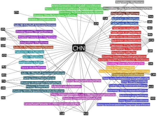
Figure 7: China in Olympic Games 2004

Figure 8: USA in Olympic Games 2004

For example, Fig.7 depicts the sports in which China has won medals as well as the correspondent competitive nations in the year 2004. Each community that China has been involved are marked as different colors. It is very intuitive that in the sports such as TableTennis, and Badminton, KOR is a strong competitor, while in Swimming and Diving, China has to compete with USA and AUS.

By contrast, Fig.8 presents the sports in which USA has won medals in the year 2004. It is apparent that most of USA’s advantage sports concentrate on swimming, Athletics, as well as Gymnastics with its major competitors such as AUS in swimming, ROU in Gymnastics, and ITA in Athletics.

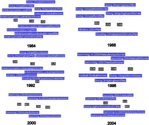
Figure 9: CHN vs. USA in Olympic Games From 1984 to 2004

Given the set of communities at time $t$, $\mathcal{C}_{t}$, for any community $\mathcal{C}_{t}^{i}\in\mathcal{C}_{t}$, if there exists at least one community $\mathcal{C}_{t+1}^{j}\in\mathcal{C}_{t+1}$, such that

$$\frac{|E(\mathcal{G}_{\mathcal{C}_{t}^{i}})\cap E(\mathcal{G}_{\mathcal{C}_{t+1}^{j}})|}{|E(\mathcal{G}_{\mathcal{C}_{t}^{i}})\cup E(\mathcal{G}_{\mathcal{C}_{t+1}^{j}})|}\geq f$$

we say $\mathcal{C}_{t+1}^{j}\in\mathcal{C}_{t+1}$ is the $descender$ of $\mathcal{C}_{t}^{i}\in\mathcal{C}_{t}$, and $\mathcal{C}_{t}^{i}\in\mathcal{C}_{t}$ evolves to $\mathcal{C}_{t+1}^{j}\in\mathcal{C}_{t+1}$. In our experiments, the empirical value of $f$ on the olympic data is set to 0.1. Fig.9 depicts the evolving trace of one community where CHN competes with USA in the sports of Diving and ArtisticGymnastics from 1984 to 2004. We see that although CHN has competed with USA in Diving:10mplatformWomen continuously for 4 Olympic Games, USA has still been keeping its advantage in water sports steadily.

5 Conclusion

In this paper, we have proposed a new method BiTector for efficient overlapping community identification in large-scale bipartitie networks. We have demonstrated the effectiveness and efficiency of BiTector over a number of real networks coming from disparate domains whose structures are otherwise difficult to understand. Experimental results show that this algorithm can extract meaningful communities that are agreed with both of the objective facts and our intuitions. BiTector avoids loss of essential information caused by the one-mode projection approach and the thresholding procedures, and is expected to be of great help in many practical scenarios.

Acknowledgments.

We thank Xin Yang for the collection of the Olympic Games data greatly.

References

- [1] Watts, D., Strogatz, S.: Collective dynamics of small-world networks. Nature 393(6684) (June 1998) 440–442
- [2] Watts, D.: Small Worlds:The Dynamics of Networks between Order and Randomness. Princeton University Press, Princeton (1999)
- [3] Girvan, M., Newman, M.: Community structure in social and biological networks. PNAS 99(12) (June 2002) 7821–7826
- [4] Newman, M.: Modularity and community structure in networks. PNAS 103(23) (June 2006) 8577–8582
- [5] Newman, M.: Detecting community structure in networks. The European Physical Journal B 38(2) (May 2004) 321–330
- [6] Palla, G., Dernyi, I., Farkas, I.: Uncovering the overlapping community structure of complex network in nature and society. Nature 435(7043) (June 2005) 814–818
- [7] Newman, M.E.J.: The structure of scientific collaboration networks. PROC.NATL.ACAD.SCI.USA 98 (2001) 404
- [8] http://www.imdb.com/
- [9] http://www.netflix.com/
- [10] Jeong, H., Tombor, B., Albert, R., Oltvai, Z.N., Barabasi, A.L.: The large-scale organization of metabolic networks. NATURE v 407 (2000) 651
- [11] Goh, K.I., Cusick, M.E., Valle, D., Childs, B., Vidal, M., Barabasi, A.L.: The human disease network. PNAS 104(21) (May 2007) 8685–8690
- [12] Girvan, M., Newman, M.: Finding and evaluating community structure in networks. Physical Review E 69(026113) (2004)
- [13] Guimera, R., Sales-Pardo, M., Amaral, L.A.N.: Module identification in bipartite and directed networks. (2007)
- [14] Barber, M.J.: Modularity and community detection in bipartite networks. Physical Review E 76 (2007) 066102
- [15] Newman, M.E.J.: Finding community structure in networks using the eigenvectors of matrices. Physical Review E 74 (2006) 036104
- [16] Lehmann, S., Schwartz, M., Hansen, L.K.: Bi-clique communities. (2007)
- [17] Fortunato, S., Barthelemy, M.: Resolution limit in community detection. PROC.NATL.ACAD.SCI.USA 104 (2007) 36
- [18] http://fimi.cs.helsinki.fi/src/
- [19] http://vlado.fmf.uni-lj.si/pub/networks/data/ucinet/ucidata.htm#davis
- [20] http://olympic.org
- [21] http://cobweb.ecn.purdue.edu/KDDCUP/data/
- [22] CCNR Resources, http://www.nd.edu/~networks/resources.htm
- [23] http://arxiv.org
- [24] http://www.netflixprize.com/download
- [25] http://www.informatik.uni-freiburg.de/~cziegler/BX/