Ratcheting Heat Flux against a Thermal Bias

Abstract

Merely rocking the temperature in one heat bath can direct a steady heat flux from cold to hot against a (time-averaged) non-zero thermal bias in stylized nonlinear lattice junctions that are sandwiched between two heat baths. Likewise, for an average zero-temperature difference between the two contacts a net, ratchet-like heat flux emerges. Computer simulations show that this very heat flux can be manipulated and even reversed by suitably tailoring the frequency ($\lesssim$ 100 MHz) of the alternating temperature field.

The generation of heat flow and its controlled manipulation presents an ever-growing endeavor for mankind. In quest of its technological solution we could witness substantial progress over the least decades, with first serious efforts being achieved that can be traced back to the early 1960’s CStarr ; Williams66 ; Eastman68 ; Thomas70 ; rectifier70 . This underlying challenge does not present plain sailing because phonons are by far more difficult to control than electrons and photons. The recent years, however, have given headway to new advances. In particular, thermal rectifiers have been designed theoretically rectifier ; diode ; quantumdiode ; Hu06 ; peyrard ; yang with a first experimental realization put forward with help of asymmetric nanotubes experimentaldiode . Moreover, using the negative differential thermal resistance diode , a thermal transistor has been proposed transistor , which is able to control heat flow much like a Field-Effect-Transistor(FET) does for electric currents. Even different thermal logic gates WangLi07 have been conceived. All this progress implies that phonons, – traditionally being regarded rather as a nuisance –, can in fact be put to work constructively in order to carry and process information effectively. Altogether, this has giving cause for a new discipline - phononics -, i.e. the science and engineering of phonons WangLi08 .

In addressing this theme let us remind again of the original formulation of the second Law by Rudolf Clausius in 1850 which states that heat cannot spontaneously flow from a subsystem at lower temperature to a coupled subsystem at higher temperature¹. Thus, in order to generate a steady heat flow against a thermal bias, or even generate heat flow in absence of a thermal bias, the system necessarily must operate away from thermal equilibrium, beyond the limiting realm of the $2$nd Law. A typical such situation that comes to mind is the Peltier effect where a steady heat flow is generated via imposing a stationary electric current across an isothermal junction of two different materials.

With this work we propose via computer simulations an intriguing new scheme that does not require the resource of a stationary non-equilibrium bias in the form of e.g. a stationary electric current but instead combines the elements of an asymmetric lattice structure with a non-biased, temporally alternating bath temperature. Dwelling on ideas from the field of Brownian motors BM1 ; BM2 ; BM3 ; BM4 , – originally devised for Brownian particle transport, – we here attempt to direct a priori energy (heat) across a spatially extended nonlinear lattice, see Fig. 1, against an external thermal bias. This objective is thus similar in spirit for devising machines and devices that can pump heat on a molecular scale vandenbroeckPRL2006 ; segalPRE2006 ; marathePRE2007 ; vandenbroeckPRL2008 . In doing so, the lattice system is brought into contact with two heat baths, with one bath subjected to a time-varying temperature. Taken alone, this nonlinear lattice structure exhibits a thermal diode effect rectifier ; diode which can be exploited to function as a heat ratchet device when an additional source of nonequilibrium, – here realized with a rocking bath temperature – , is present. Then, merely rocking the temperature in one heat bath can induce dynamically a finite bias between the two heat baths, being held at the same time-averaged temperature. This novel nonequilibrium ratchet feature can be utilized (i) to reverse the flux, to (ii) direct heat flow from cold to hot against an average thermal bias, or even to (iii) turn a regime with a negative differential thermal resistance (NDTR) into a regime with positive DTR, and vice versa.

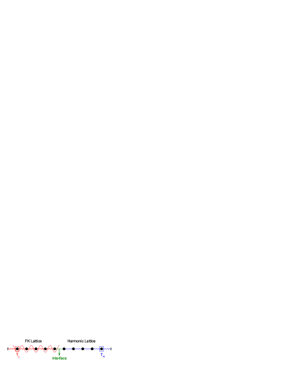
Figure 1: (Color-online) Schematic setup of a weakly coupled Frenkel-Kontorova lattice to a Harmonic lattice, being coupled to two heat baths at temperatures $T_{L}(t):=T_{L}$ and $T_{R}$.

Explicitly, we study numerically a system composed of a Frenkel-Kontorova (FK) nonlinear lattice of period $a$ which is weakly coupled to a Harmonic lattice (HL), each consisting of $N/2$ atoms of identical mass $m$. This setup is shown in Fig. 1, with the FK lattice on the left and Harmonic lattice on the right. The FK-HL configuration is governed by the Hamiltonian:

$$H=\sum^{\frac{N}{2}}_{i=1}\left[\frac{p^{2}_{i}}{2m}+\frac{k_{L}}{2}(q_{i}-q_{i-1})^{2}-\frac{V_{L}}{(2\pi)^{2}}\cos\frac{2\pi q_{i}}{a}\right]$$

$$+\frac{k_{int}}{2}(q_{\frac{N}{2}+1}-q_{\frac{N}{2}})^{2}+\sum^{N}_{i=\frac{N}{2}+1}\left[\frac{p^{2}_{i}}{2m}+\frac{k_{R}}{2}(q_{i+1}-q_{i})^{2}\right]$$ (1)

Herein, $q_{i}=x_{i}-ia$ denotes the displacement from equilibrium position $ia$ for $i$-th atom, $a$ is the lattice period, $k_{L}$ and $V_{L}$ are the spring constant and the on-site potential of the FK lattice, $k_{int}$ is the coupling strength between the FK and the Harmonic lattice, and $k_{R}$ is the spring constant of the Harmonic lattice. Fixed boundary conditions, yielding $q_{0}=q_{N+1}=0$, have been employed. The $1$-st atom and the $N$-th atom are put into contact with two Langevin heat baths possessing temperature $T_{L}(t):=T_{L}$ and $T_{R}$, respectively. Gaussian white noise are used, namely, $\langle\xi_{1/N}(t)\rangle=0$ and $\langle\xi_{1/N}(t)\xi_{1/N}(0)\rangle=2k_{B}\eta T_{L/R}\delta(t)$. $k_{B}$ is the Boltzmann constant and $\eta$ denotes the coupling strength between system and heat bath. The time-varying heat bath temperature $T_{L}(t)$, oscillates dichotomously at angular frequency $\omega$ and driving strength $A$. The used bath temperatures thus read explicitly:

$$T_{L}(t):=T_{L} = T_{0}(1+\Delta+A\cdot\text{sgn}(\sin{\omega t})),$$

$$T_{R} = T_{0}(1-\Delta)\;,$$ (2)

where $T_{0}=(\overline{T_{L}(t)}+T_{R})/2$ is the temporally averaged environmental reference temperature, $2\Delta=(\overline{T_{L}(t)}-T_{R})/T_{0}$ denotes the normalized temperature difference, and $\text{sgn}(\sin{\omega t})$ provides the dichotomous, time-dependent temperature variation. The time scale $\omega$ of the temperature manipulation of the heat bath is assumed to vary much slower than the time scale $\tau_{leq}$ to reach local thermal equilibrium; i.e. $\omega<<\tau^{-1}_{leq}$. This time scale for good thermal conductors is typically a function of temperature; it is of the order of the time scale of the electron-phonon relaxation time which normally decreases with decreasing temperature. For good metals this time scale is of the order of $0.1-1$ picoseconds.

We next use dimensionless parameters by measuring positions in units of $a$, momenta in units of $[a(mk_{L})^{1/2}]$, temperature in units of $[k_{L}a^{2}/k_{B}]$, spring constants in units of $k_{L}$, frequencies in units of $[(m/k_{L})^{1/2}]$ and energies in units of $[k_{L}a^{2}]$. In particular, we set in our simulations $k_{L}=1,V_{L}=5,k_{int}=0.05,k_{R}=0.2$. For a typical situation, the dimensionless temperature is set at $T_{0}=0.09$. This yields with $k_{L}a^{2}/k_{B}\sim 10^{3}K-10^{4}K$ a physical temperature of the order $T_{0}\sim 90K-900K$. The equations of motion are integrated by the symplectic velocity Verlet algorithm with a small time step $h=0.005$. The system is simulated for a total time $tt=2\cdot 10^{8}$. The chosen optimal coupling strength of the heat bath is fixed at $\eta=0.5$.

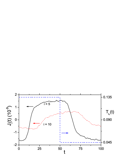
Figure 2: (Color Online) The numerically ($10^{6}$ realizations) evaluated, periodically varying asymptotic local heat flux $J_{i}(t)$ over the full driving period $2\pi/\omega=100$ is compared with the rocking bath temperature $T_{L}(t)$, at driving strength $A=0.5$ and zero bias $\Delta=0$ for $T_{0}=0.09$. The lattice length is $N=50+50$. The numerically cycle averaged, spatially homogenous heat flux equals $J=-4.92\cdot 10^{-6}$($i=5$) and $J=-4.93\cdot 10^{-6}$ ($i=10$).

The asymptotic heat flux $J_{i}(t)$ is assuming the periodicity of the external driving period $2\pi/\omega$ after the transients have died out. This fact is assured for all of our chosen frequencies $\omega$ after a simulation time of $st\sim O(10^{7})$. At those asymptotic long times $t$ the heat flux equals the noise average $J_{i}(t)=k_{i}\left\langle\dot{q}_{i}(q_{i}-q_{i-1})\right\rangle$ where $k_{i}=k_{L}$ for $i=2,\dots,N/2$ and $k_{i}=k_{R}$ for $i=(N/2)+2,\dots,N$, being here evaluated in the commonly employed way, cf. in Refs. rectifier ; diode ; Hu06 ; peyrard ; yang ; transistor ; lepri . The static heat flux $J$ then follows as the cycle average over a full temporal period: $J=\frac{\omega}{2\pi}\int_{0}^{2\pi/\omega}J_{i}(t)dt$, which with ergodicity being valid equals as well the long time average, i.e. $J=k_{L}\overline{\dot{q}_{2}(q_{2}-q_{1})}=k_{R}\overline{\dot{q}_{N}(q_{N}-q_{N-1})}$. In Fig. 2 we depict the resulting periodic variation of the heat flux $J_{i}(t)$ vs. the externally applied temperature variation $T_{L}(t)$. This nonlinear response exhibits a characteristic phase lag vs. the perturbation $T_{L}(t)$ and is dynamically biased to yield a nonzero temporal average.

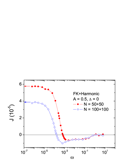
Figure 3: (Color-online) Time averaged heat flux $J$ vs. the angular driving frequency $\omega$ for different lattice lengths $N=50+50$ and $N=100+100$ and $T_{0}=0.09$. The two arrows mark the heat flux calculated in the adiabatic limit.

With the introduction of a temporally alternating temperature field in Eq. (Ratcheting Heat Flux against a Thermal Bias), we thus achieve a controllable manipulation of heat flow by an externally adjustable parameter, i.e. the driving frequency $\omega$. The static thermal bias $\Delta$ has been set to zero. The only resource driving heat across the junction thus is the non-equilibrium, alternating temperature field $T_{L}(t)$, which generates positive and negative temperature variations in the first and second half of driving period. As a result, the direction of heat flow will tend to reverse each half driving period. In the adiabatic limit; i.e. $\omega\rightarrow 0$, the alternating temperature $T_{L}(t)$ can be expressed by two opposite static thermal bias values, yielding the average heat current approximately as the averaged heat current for two opposite static thermal bias values, see the two horizontal arrows depicted in Fig. 3. In contrast, in the fast-driving limit $\omega\rightarrow\infty$, the left-end atom will experience a time-averaged constant temperature. This corresponds to thermal equilibrium, yielding $J\rightarrow 0$ when $\omega\rightarrow\infty$. In Fig. 3, the numerically determined average heat current is depicted as a function of the driving frequency $\omega$ for the driving amplitude $A=0.5$. In full agreement with our predictions, a finite heat current $J$ emerges in the adiabatic limit $\omega\rightarrow 0$, becomes diminished in the non-adiabatic limit and essentially vanishes for large $\omega$. At adiabatic driving the values of $J$ agree well with the numerical values determined from the adiabatic approximation. A tantalizing observation is that $J$ does not vanish monotonically. Remarkably, at some intermediate value $\omega$, the heat flow $J$ crosses zero and subsequently reverses its direction upon further increasing $\omega$. Consequently, the direction of net heat flow can be manipulated by suitably tailoring the frequency of the temperature variations.

This interesting reversal of the heat flux can be related to the thermal response time of the system. The non-rocked FK lattice obeys Fourier’s law HuLiZhao . Thus, the corresponding temperature variations $T(t,x)$ obey the diffusion equation: $\partial{T}/\partial{t}=(\kappa/c)\partial^{2}{T}/\partial{x^{2}}$, where $\kappa$ denotes the heat conductivity and $c$ is the specific heat. The solution follows a Gaussian wave packet $T(t,x)=1/2\sqrt{\pi\kappa t/c}\exp(-x^{2}c/4\kappa t)$. The thermal response time can now be estimated as the time span for the energy to diffuse across the system, i.e. $\tau\sim cN^{2}/4\kappa$. At temperature $T_{0}=0.09$, the FK lattice assumes the numerical values $\kappa\sim 0.5$ and $c\sim 1$. Thus, the characteristic frequency scale $\omega_{c}$ of the system can be estimated as $\omega_{c}=2\pi/\tau$. This characteristic frequency scales inversely with the system size $\propto N^{-2}$. For $N=100$ we then find $\omega_{c}\sim 10^{-3}$ and a roughly four times smaller value for $N=200$. These two estimates for $\omega_{c}$ are in good agreement with those observed numerically in Fig. 3. Taking the physical unit of frequency, i.e. $\omega_{0}=[(m/k_{L})^{1/2}]\sim 10^{13}\,\text{sec}^{-1}$ into account, $\omega_{c}\sim 10^{-3}$ corresponds to a typical physical frequency for microwaves of $\sim 10^{10}\,\text{sec}^{-1}$. The theoretically predicted red shift $\propto N^{-2}$ for $\omega_{c}$ with increasing system size is nicely corroborated by our numerical results.

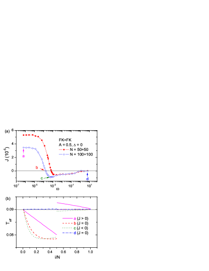
Figure 4: (Color-online) (a) Stationary heat flux $J$ vs. driving frequency $\omega$ for different lattice lengths $N=50+50$ and $N=100+100$ at $T_{0}=0.09$ and a driving strength $A=0.5$. (b) The effective temperature profiles of four selected points in (a) at length $N=100+100$.

To gain additional insight into this reversal of heat flow we investigate the local temperature variations across the junction at different driving frequencies $\omega$. After evolving the system over a long total simulation time $tt=2\cdot 10^{8}$ this local temperature of $i$-th atom is evaluated from its temporal long time average of the kinetic energy, i.e. $T_{eff}(i)=\overline{\dot{q}^{2}_{i}}$. In doing so, we switch to a FK-FK configuration because the harmonic lattice knowingly is not able to build up a temperature gradient lepri . The employed right sided FK lattice has the parameters $(k_{R}=0.2,V_{R}=1)$. In Fig. 4(a) a similar heat current modulation as for the FK-HL configuration is observed for the FK-FK junction with $\Delta=0$ and $A=0.5$. The effective temperature profiles of four numerical runs, denoted as (a,b,c,d) in Fig. 4(a), are depicted in Fig. 4(b) versus the relative site positions $i/N$.

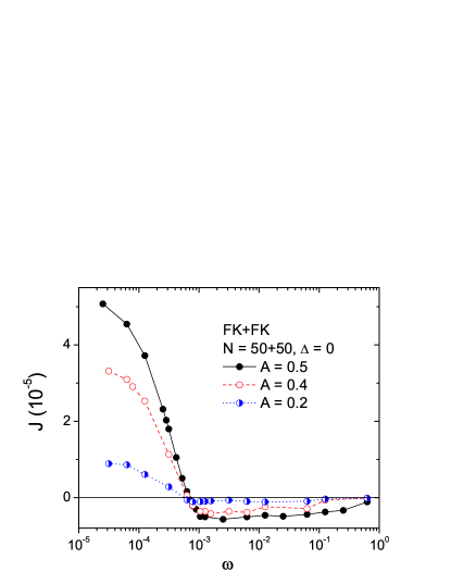
Figure 5: (Color-online) Stationary heat flux $J$ vs. driving frequency $\omega$ for different driving strengths $A$ of the temperature modulation for a size $N=50+50$ at $T_{0}=0.09$ and zero thermal static bias $\Delta$.

In clear contrast to a non-rocking case (i.e. $A=0$) with no net temperature bias, a distinct temperature gradient now emerges for a rocking temperature $T_{L}(t)$. The temperature profile exhibits a discontinuity at the interface. For the situation in (c) where the heat flow reversal $J$ approaches its lowest, negative value, the effective temperature profile becomes rather complicated: Away from the bending part (with a negative-valued slope) towards the left terminal side the resulting temperature profile exhibits an opposite thermal gradient in comparison to case (a)–thus indicating that a current reversal occurs. This opposite thermal gradient behavior can also be detected upon comparing the temperature gradients of case (b) and (d), exhibiting both a vanishing heat flow $J=0$. The discontinuity of $T_{eff}(i)$ occurring at the interface reaches its maximal value at low frequencies, cf. case (a), and increasingly diminishes with increasing driving frequency beyond the frequency value for reversal, cf. case (d).

We next investigated numerically the role of the driving strength $A$ of the temperature modulation versus driving frequency $\omega$. The results are depicted with Fig. (5). As expected, a lower driving strength consistently yields smaller values of the Brownian motor induced heat flux $J$, which vanishes identically when the strength of the source of nonequilibrium is approaching zero, i.e. $A=0$. Because the frequency scale $\omega_{c}$ for occurrence of heat flux reversal is mainly size dependent $\propto N^{-2}$ we expect a weak dependence of $\omega_{c}$ on driving strength $A$. This result is corroborated with Fig. (5) where this characteristic frequency is practically independent of driving strength $A$.

Flux-bias characteristics. The finite ratchet value of heat flux $J$ in the absence of static thermal bias $\Delta$ now allows for directing heat current against a non-zero thermal bias $\Delta$. In Fig. 6, we depict the flux-bias characteristics $J-\Delta$ at small driving frequency $\omega=1.571\cdot 10^{-5}$ ($\sim 100$ MHz), which is in the range of ultrasonic frequencies. The $J-\Delta$ curve in absence of time-dependent manipulation ($A=0$) is presented as a reference, obeying $J(\Delta=0)=0$, in agreement with the $2$nd Law. The dashed line corresponds to a driving amplitude $A=0.5$. We now detect a finite heat current $J$ at vanishing thermal bias $\Delta=0$. For negative bias within the range $\Delta\in[-0.23,0]$, the direction of the heat flow is positive. With $J$ taken as the average over a driving period this implies that heat flows from cold to hot. The so called “stall bias” of the thermal bias that yields $J=0$ is located around $\Delta=-0.23$. Moreover, we detect that the characteristics of (NDTR) becomes modified as well by the switch-on of the alternating bath temperature $T_{L}(t)$. The original working range of NDTR at $A=0$ is $\Delta\in[-0.6,-0.2]$. At $A=0.2$, this range undergoes a shift towards $\Delta\in[-0.7,-0.3]$. For $A=0.5$, this very NDTR-phenomenon effect can be dynamically eliminated all together. This effect is thus of prominent interest for the design of a efficient thermal transistor: It allows one to change the range of working temperatures of a thermal transistor by solely adjusting the strength of the driving temperature field.

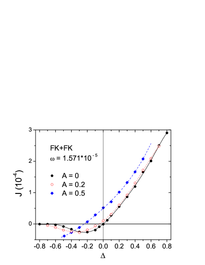
Figure 6: (Color-online) Heat flux $J$ vs. thermal bias $\Delta$ for different driving amplitudes $A=0,\,0.2$, and $0.5$. The lattice length is $N=50+50$ and $T_{0}=0.09$. Note that the nonlinearity in the Frenkel-Kontorva part of the junction is essential to obtain the thermal ratchet effect. At large rocking strength ($A=0.5$) the current-bias characteristics can be manipulated to eliminate a NDTR-regime at negative bias values $\Delta$.

In conclusion, we have shown that heat flow across a structured nonlinear lattice junction can be efficiently controlled by use of a temporally alternating temperature field. The heat flow becomes directed and even can be reversed by suitably selecting the driving frequency. In clear contrast to the thermal diode effect, the presented Brownian heat rachet physics dynamically generates a finite heat flux at zero thermal bias $\Delta=0$. Thus, we deal with a new phenomenon which, as well, is in distinct contrast to the by now common situation of thermally assisted, directed particle transport in Brownian motors BM1 ; BM2 ; BM3 ; BM4 . This dynamically induced heat flow can be directed against a non-zero, time-averaged net thermal bias $\Delta$. This fact, however, does not necessarily imply an active overall cooling of the device, cf. also Fig. 4 (b). The size and the shape of NDTR can be manipulated as well. Nonlinearity, as reflected with the FK-segment, is essential for the phenomenon: a junction composed of two asymmetric harmonic lattices fails to support a rachet heat flux. All these phenomena call for beneficial applications in the control and management of heat flow on the micro- and nano-scale. With a future, more detailed work future we shall investigate, how the size of the directed heat flux can be enlarged by stylizing further the nonlinearity of the lattice structure. In particular, we expect much larger heat currents when using a Fermi-Pasta-Ulam chain containing both, a cubic and a quartic interaction potential.

Our setup constitutes a two-segment rectifier model diode and the driving frequency is in a range of ($\lesssim 100$ MHz). The finite, directional heat flux is feasibly detected by slowly rocking the bath temperature within the adiabatic regime. Given the fact that rectification has been demonstrated experimentally in asymmetrically deposited nanotubes experimentaldiode , we are confident that the appealing heat ratchet phenomena presented herein will invigorate experimentalists to validate our findings by designing such thermal ratchet systems.

- (1) C. Starr, J. Appl. Phys. 7, 15 (1936).
- (2) A. Williams, Ph.D Thesis, Manchester University (1966).
- (3) G. Y. Eastman, Sci. Am. 218, 38 (1968).
- (4) T. R. Thomas and S. D. Probert, Int. J. Heat Mass Transfer, 12, 789 (1970).
- (5) P. W. O’Callaghan, S. D. Probert, and A. Jones, J. Phys. D 3, 1352 (1970).
- (6) M. Terraneo, M. Peyrard, and G. Casati, Phys. Rev. Lett. 88, 094302 (2002).
- (7) B. Li, L. Wang, and G. Casati, Phys. Rev. Lett. 93, 184301 (2004).
- (8) D. Segal and A. Nitzan, Phys. Rev. Lett. 94, 034301 (2005).
- (9) B. Hu, L. Yang, and Y. Zhang, Phys. Rev. Lett. 97, 124302 (2006).
- (10) M. Peyrard, Europhys. Lett. 76, 49 (2006).
- (11) N. Yang, N. Li, L. Wang, and B. Li, Phys. Rev. B 76, 020301(R) (2007).
- (12) C. W. Chang, D. Okawa, A. Majumdar, and A. Zettl, Science 314, 1121 (2006).
- (13) B. Li, L. Wang, and G. Casati, Appl. Phys. Lett. 88, 143501 (2006).
- (14) L. Wang and B. Li, Phys. Rev. Lett. 99, 177208 (2007).
- (15) L. Wang and B. Li, Physics World 21 (3), 28 (2008).
- (16) P. Reimann et al., Phys. Lett. A 215, 26 (1996).
- (17) R. D. Astumian and P. Hänggi, Phys. Today 55 (11), 33 (2002).
- (18) P. Hänggi, F. Marchesoni, and F. Nori, Ann. Phys. (Leipzig) 14, 51 (2005).
- (19) P. Reimann and P. Hänggi, Appl. Phys. A 75, 169 (2002).
- (20) C. Van den Broeck, Phys. Rev. Lett. 96, 210601 (2006).
- (21) D. Sigal and A. Nitzan, Phys. Rev. E 73, 026109 (2006).
- (22) R. Marathe, A. M. Jayannavar and A. Dhar, Phys. Rev. E 75, 030103(R) (2007).
- (23) M. van den Broeck and C. Van den Broeck, Phys. Rev. Lett. 100, 130601 (2008).
- (24) S. Lepri, R. Livi, and A. Politi, Phys. Rep. 377, 1 (2003).
- (25) B. Hu, B. Li, and H. Zhao, Phys. Rev. E 57, 2992 (1998).
- (26) C.J. Thompson, Classical Equilibrium Statistical Mechanics, (Calendron Press, Oxford 1988).
- (27) N. Li, P. Hänggi, and B. Li, extended version, in preparation.