Polaris the Cepheid returns:
$4.5$ years of monitoring from ground and space

Abstract

We present the analysis of $4.5$ years of nearly continuous observations of the classical Cepheid Polaris, which comprise the most precise data available for this star. We have made spectroscopic measurements from ground and photometric measurements from the wire star tracker and the smei instrument on the coriolis satellite. Measurements of the amplitude of the dominant oscillation ($P=4$ d), that go back more than a century, show a decrease from $A_{V}=120$ mmag to $30$ mmag around the turn of the millennium. It has been speculated that the reason for the decrease in amplitude is the evolution of Polaris towards the edge of the instability strip. However, our new data reveal an increase in the amplitude by $\sim 30\%$ from 2003–2006. It now appears that the amplitude change is cyclic rather than monotonic, and most likely the result of a pulsation phenomenon. In addition, previous radial velocity campaigns have claimed the detection of long-period variation in Polaris ($P>40$ d). Our radial velocity data are more precise than previous datasets, and we find no evidence for additional variation for periods in the range 3–50 d with an upper limit of 100 m s^-1. However, in the wire data we find evidence of variation on time-scales of 2–6 days, which we interpret as being due to granulation.

1. Introduction

In addition to being arguably the most famous and in practice useful star other than the Sun, Polaris has a number of properties that may provide insights that are important to stellar astrophysics. It is the nearest and brightest classical Cepheid, oscillating in a single mode of pulsation with a period around four days. The hipparcos parallax constrains its luminosity and allowed Feast & Catchpole (1997) to argue that the mode of pulsation must be the first overtone, which is upheld by the recent reevaluation of the hipparcos data (van Leeuwen et al., 2007). As discussed by Evans et al. (2002), Polaris has a number of unusual pulsation properties, including a very small pulsation amplitude, and, as for other overtone pulsators, it has a rapid period change. It has been clear from studies as far back as Parenago (1956) and Szabados (1977) that overtone pulsators (“s Cepheids” as they were then called) had rapid period changes, more rapid than can be explained by evolution during a second or third crossing of the instability strip.

It was found by Arellano Ferro (1983) that the main period of Polaris is increasing (316 s per century) and that its peak-to-peak amplitude has decreased significantly, from about 140 to 70 mmag (Johnson $B$ filter), based on photoelectric measurements collected in the period 1930–1980. Kamper & Fernie (1998) analysed radial velocity measurements from 1900 to 1998 and could confirm the decrease in amplitude. However, their radial velocity data from the end of the period showed that the decrease had apparently stopped. Turner et al. (2005) analysed both radial velocity and photometry data and found evidence for a sudden change in oscillation period around 1963–1966, and that the amplitude change became steeper at the same time.

Our aim is to shed light on the properties of the oscillation of Polaris, based on the analysis of a nearly continuous dataset spanning $4.5$ years. We have photometry from two satellite missions and simultaneous spectroscopic monitoring from the ground, each dataset being superior to previous data available for Polaris.

Table 1Observing log. The point-to-point scatter, $\sigma$, is given in mmag (wire $+$ smei photometry) and km s^-1 (spectroscopy).

				Data
Source	Date start	Date end	$T_{\rm obs}$ [d]	points	$\sigma$
wire	2004 Jan 17	2004 Feb 15	29.0	41 162	0.88
wire	2004 Jul 10	2004 Jul 30	20.2	33 937	0.30
wire	2005 Jan 31	2005 Feb 12	12.6	14 240	0.29
smei	2003 Apr 6	2006 Dec 31	1365.4	13 543	6.4
ast	2003 Dec 25	2007 Oct 26	1401.0	517	0.15
D89	1987 May 6	1988 Jan 3	241.0	175	0.44
H00	1991 Nov 21	1993 Aug 2	640.4	42	0.07

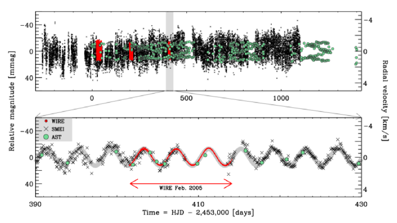
Figure 1.— The photometry datasets from smei and wire and the radial velocities from ast. The bottom panel is an expanded view of 40 days of observations surrounding the last run with wire. The thick gray curve is the fit of a single sinusoid to the smei data.

2. Observations and data reduction

Polaris ($\alpha$ Ursae Minoris) was observed with the star tracker on the Wide-field InfraRed Explorer (wire; Bruntt 2007) satellite in January and February 2004, July 2004, and February 2005. These runs lasted about 4, 3 and 2 weeks, respectively. In addition, Polaris was monitored using 3.8 years of nearly continuous photometry from the smei instrument on the coriolis satellite. These observations were obtained between April 2003 and the end of 2006. We further used the 2 m Tennessee State University Automatic Spectroscopic Telescope (AST; Eaton & Williamson 2004, 2007) to collect 517 high dispersion spectra of Polaris over a period of $3.8$ years, from late 2003 to late 2007. A log of the photometric and radial velocity observations is given in Table 1. We also list datasets from two previous radial velocity campaigns that we have used for comparison in our analysis in Sect. 5 (D89: Dinshaw et al. 1989 and H00: Hatzes & Cochran 2000).

The complete photometric light curve from smei and wire and the radial velocity data from ast are shown in the top panel in Fig. 1. Note that different units for the photometry (mmag) and velocities (km s^-1) are given on the left and right abscissa, respectively. The right abscissa is adjusted by the ratio of the measured amplitudes in the ast spectroscopy and the smei photometry. The bottom panel in Fig. 1 shows the details of the variation during 40 days. It shows the last run done with wire and illustrates the typical coverage with smei and the ast. The thick gray curve is the fit of a single sinusoid to the complete smei dataset.

Table 2Times of maximum light in the smei and wire datasets.

$t_{E}$	Epoch	Source
[HJD $-2,453,000$]
$391.327$	6329	smei
$395.339$	6330	smei
$399.387$	6331	smei
$403.323$	6332	wire
$407.274$	6333	wire
$411.262$	6334	wire
$415.418$	6335	smei
$419.160$	6336	smei
$423.215$	6337	smei
$427.152$	6338	smei

The wire dataset consists of about three million CCD stamps extracted from the 512$\times$512 CCD SITe star tracker camera. Each window is 8$\times$8 pixels and we carried out aperture photometry using the pipeline described by Bruntt et al. (2005). The resulting point-to-point scatter range from $0.3$ to $0.9$ mmag (see Table 1). The noise is somewhat higher than the Poisson noise, e.g. the high noise in the first wire dataset is due to a high background sky level.

Data from the ast consist of échelle spectra covering the wavelength range $5\,000$–$7\,100$ Å at a resolution of about $30\,000$. The velocities are derived from the correlation between the observed spectrum and a list of 74 mostly Fe i lines. More details about the pipeline used to extract the radial velocities are given by Eaton & Williamson (2007). We find that the velocities deviate slightly from the IAU velocity system ($\Delta v=-0.35\pm 0.09$ km s^-1). The drift of the velocities due to the motion of Polaris in its binary orbit (Kamper, 1996) was subtracted before the time-series analysis was carried out.

The Solar Mass Ejection Imager (smei) (Eyles et al., 2003; Jackson et al., 2004) is a set of three cameras mounted on the side of the coriolis satellite. Each camera covers a $3\times 60$ degree strip of sky and this is projected onto $1260\times 40$ pixels of a CCD. As the nadir-pointing satellite orbits every 101 minutes in its Sun-Synchronous polar orbit the cameras take continuous 4-second exposures, which result in roughly 4,500 images per orbit covering most of the sky. After bias and dark removal and flat-fielding processing, the pixels about the target star are selected from about ten images that contain the star for each orbit. These pixels are then aligned and a standard PSF is fitted by least-squares. Thus, the result is one brightness measure every 101 minutes. There are problems with particle hits and a complex PSF, which shows temporal variations that are not fully understood. The short-term ($t<1.0$ d) accuracies are of the order of a few mmag, but there are longer term systematic errors of the order of 10 mmag on the timescales of days and months, which are not yet well understood. Allowing for time allocated for calibrations and satellite operation, a time coverage of about 85% was maintained.

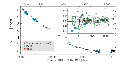
Figure 2.— $O-C$ diagram. The solid line is a fit to the data taken after 1965. The inset shows the details of the new $O-C$ data from smei and wire.

3. Period change of the main mode

Observed epochs of maximum light in Polaris, spanning more than a century, have indicated a significant change in period (Arellano Ferro, 1983; Fernie et al., 1993; Turner et al., 2005). These studies have considered $O-C$ diagrams and fitted a parabola, which is equivalent to assuming the period changes linearly with time. We have combined new measured epochs with those from Turner et al. (2005). A sudden change in the period has been noted in the 1960’s and therefore we have only used epochs observed since 1965.

We measured 223 and 16 epochs of maximum light in the smei and wire datasets, respectively. From the $O-C$ analysis by Arellano Ferro (1983) we expected the period to decrease by 14 seconds over the $4.5$ years time span of our dataset. Thus, when predicting the epochs of maximum light we could safely assume a constant period. The epochs were predicted by fitting a single sinusoid to the smei data. The fit is of the form $S(t)=A\sin[2\pi(f\,(t-t_{0})+\phi)]$, where $A$ is the amplitude, $t$ is the time (Heliocentric Julian Date), $t_{0}$ is the zero point, $P=1/f$ is the period, and $\phi$ is the phase. The result is $P=3.972111\pm 0.000054$ days and phase $\phi=0.2158\pm 0.0022$ for the zero point $t_{0}=2,530,000$. This fit is shown with a thick gray line in the bottom panel in Fig. 1. The uncertainties were determined from simulations as discussed in Sect. 4.1.

At each epoch, $E$, we selected all data points within half a period ($|t-E*P|<P/2$). For the smei data we required that at least 30 data points were available with at least 10 data points before and after the maximum. To estimate the time of maximum light, we fitted these data with a sinusoid with fixed frequency and amplitude, while the phase was a free parameter. In Table 2 we list these times, including the epoch number following the definition by Turner et al. (2005), and the source of the data. The complete table is available in the on-line version of the paper, while the times listed here correspond to the time interval covered in the bottom panel in Fig. 1.

Since the quality of the three datasets are very different, we computed weights based on the uncertainty of the epoch times, $t_{E}$. This was determined by calculating the point-to-point scatter after subtracting a parabola fitted to the $O-C$ data of each dataset. The uncertainty on $t_{E}$ from Turner et al. (2005) is $\sigma(t_{E})=0.18$ d while for smei and wire data the uncertainties are 0.12 d and 0.014 d. Finally, we calculate the $O-C$ values using weights, $1/\sigma^{2}(t_{E})$, and the most accurate value of the period, which is the one from smei: $O-C=(t_{E}-t_{0})-(E-E_{0})\cdot P_{\rm SMEI}$. We chose the reference epoch to be $E_{0}=6333$, and using the fit to the smei data found above, this corresponds to the time $t_{0}=2,453,407.277\pm 0.009$.

Our final $O-C$ diagram is shown in Fig. 2. The recent data continue to match the smooth period change as indicated by the weighted parabolic fit, corresponding to a period increase of $dP/dt=365\pm 27$ sec/century. We note that the most recent smei data lie systematically below the fit, which is tightly constrained by the extremely well-defined times from wire. Note that if we only use data more recent than 1985, we conclude that the period has not changed, i.e. $dP/dt=-19\pm 95$ sec/century.

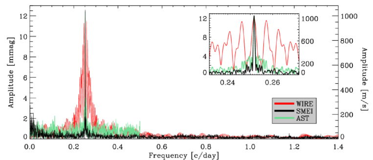
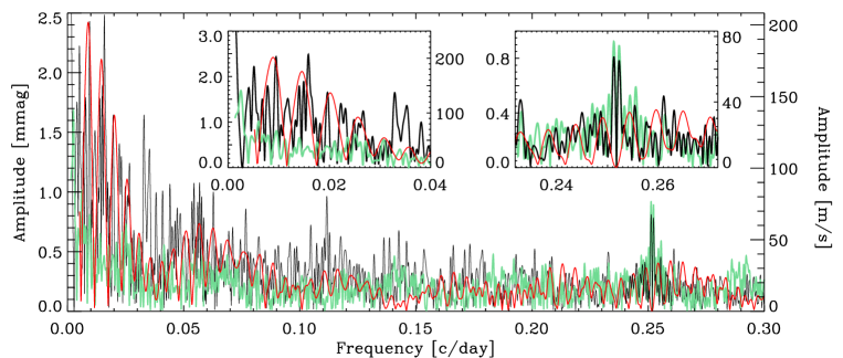
Figure 3.— Amplitude spectra of the ast radial velocity data and the photometric data from smei and wire. The top panel is for the raw data and the bottom panel is after subtracting the main mode at $\simeq 0.25$ c day^-1. The insets show details of the amplitude spectra.

Table 3Results of the frequency analysis for the five datasets.

Source	$f$ [c day-1]	$a$ [mmag/km s-1]	$\phi$ [0..1]
wire	$0.251732(14)$	$12.26(18)$	$0.2195(34)$
smei	$0.2517553(34)$	$12.63(13)$	$0.2158(22)$
ast	$0.2517506(43)$	$0.998(14)$	$0.1550(34)$
D89	$0.25174(14)$	$0.808(58)$
H00	$0.251722(22)$	$0.781(22)$

4. Amplitude change of the main mode

To analyse the time series in the frequency domain, we calculated the Fourier amplitude spectra for each dataset. In the top panels in Fig. 3 we show the amplitude spectra for the photometry from the wire (red) and smei (green) and the radial velocities from ast (black). The inset shows the prominent peak around 0.25 c day^-1, corresponding to the known 4-day period. Due to the long gaps between the three wire datasets the spectral window shows a more complex pattern than the nearly continuous datasets from smei and ast.

We fitted a single sinusoid to the dominant peak and the results for each dataset are given in Table 3. We list the phase of the wire, smei and ast datasets, relative to the zero point $t_{0}=2,453,000$. It is seen that the frequencies are in very good agreement. Although the point-to-point precision of the wire data is superior, the long span of the smei and ast datasets means the frequency is determined more accurately by a factor of 3–4. We also note that the phases from the fit to the smei and wire photometry are in good agreement, but the phase of the fit to the ast data is quite different. This corresponds to a shift in the times of maximum in the flux and radial velocity: ${\rm HJD}(F_{\rm max})={\rm HJD}(RV_{\rm max})+(1.744\pm 0.016\,{\rm d})$. In comparison, Moskalik & Ogłoza (2000) found the offset to be $1.682\pm 0.017\,{\rm d}$ using combined photometry and radial velocity data from Kamper & Fernie (1998). The shifts appear to be marginally different ($2.7\,\sigma$), but we note that the combined Kamper & Fernie (1998) data is calibrated to Johnson $V$, while smei has a filter response roughly centered at Johnson $R$ but being wider (Tarrant et al., 2007).

We have subtracted the main oscillation mode and the residual amplitude spectra are shown in the bottom panel in Fig. 3. All spectra show a higher amplitude towards lower frequencies. This could be either due to instrumental drift or long-period variation intrinsic to Polaris, which we discuss in Sect. 5. The left inset shows that the peaks in the smei data do not coincide with peaks in the ast data, so we cannot claim they are due to coherent pulsations. The right inset shows the details around $0.25$ c day^-1, where two significant residual peaks are seen in the smei and ast datasets. They are an indication that the frequency, amplitude or phase of the oscillation has changed during the $\sim 4$ years of observation.

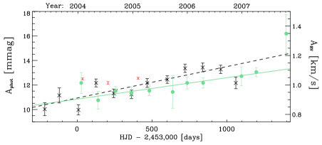
Figure 4.— Increase in the amplitude of the 4 d main mode measured over $4.5$ years with wire (small dots), smei ($\times$), and ast ($\bullet$).

To test the possible change in either frequency, amplitude or phase of the main mode, we divided the datasets into subsets. Each of the smei and ast subsets contain 30 pulsation cycles, and the three wire datasets were analysed independently. Each subset is fitted by a single sinusoid and we analysed the output parameters. We made the analysis for two different assumptions:

• We assumed that the frequency, amplitude and phase change with time, so each is a free parameter.

• We assumed that only the amplitude changes with time, so the frequency and phase were held fixed.

The first assumption allowed us to test the stability of the mode. We found that within the uncertainties both the frequency and phase do not change over the time span of the observations. However, the amplitude increases monotonically, and this result is confirmed by the analysis under the second assumption. A comparison of the measured amplitudes under the two assumptions give nearly identical amplitudes for all subsets.

In Fig. 4 we show the result obtained under the second assumption, i.e. for fixed frequency and phase. The $\times$ symbols are the smei data, the $\bullet$ symbols are the ast data, and small dots are for the three wire runs. The dashed line is a weighted linear fit to the smei data yielding the amplitude change in mmag: $A_{\rm phot}(t)=(10.94\pm 0.08)+(2.56\pm 0.13)\cdot 10^{-3}(t-t_{0})$, where $t$ is the HJD with zero point $t_{0}=2,453,000$. The weighted fit to the ast data (solid line) gives: $A_{RV}(t)=(0.90\pm 0.01)+(1.45\pm 0.15)\cdot 10^{-4}(t-t_{0})$ km s^-1. From this analysis we find that from 2003–7 the amplitude measured in flux and radial velocity has increased by $34\pm 2$% and $24\pm 3$%, respectively. The single mode in Polaris has very low amplitude and from linear theory it is expected that the rate of increase is the same in photometry and radial velocity. The measured increase over four years is only marginally different ($8.1\pm 3.1$% or $2.6\,\sigma$), and continued monitoring is required to confirm this tentative result.

In Fig. 5 the measured peak-to-peak amplitudes in radial velocity from ast are compared with results from the literature. Kamper & Fernie (1998) found a monotonic decrease in the amplitude over the past 100 years To avoid confusion about the conversion factor, we compare our results directly in radial velocity, and we have reproduced their fit as the solid black line. The dashed line is an extrapolation, and as noted by Kamper & Fernie (1998), zero amplitude would be predicted in the year 2007. However, from four years of monitoring (1993.15–1996.96) in radial velocity, Kamper & Fernie (1998) found that the peak-to-peak amplitude was nearly constant. This is in agreement with the amplitudes we find from the analysis (see Sect. 5.1) of the datasets by Dinshaw et al. (1989) and Hatzes & Cochran (2000). From the most recent high-precision data, it is evident that the amplitude in Polaris was constant in the period 1987–1997, while the increase we report here marks a new era in the evolution of Polaris.

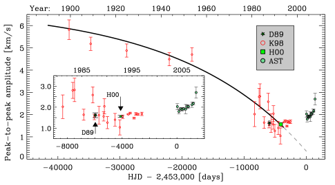
Figure 5.— Peak-to-peak radial velocity amplitude for the main 4 d mode. The solid line is the fit from Kamper & Fernie (1998). The inset shows the most recent data in detail. Our measurements of the amplitude based on the Dinshaw et al. (1989) and Hatzes & Cochran (2000) are marked by arrows.

4.1. Uncertainties in frequency, amplitude and phase

The uncertainties in the frequency, amplitude and phase in Table 3 are determined from realistic simulations of each dataset. The times of observation are taken from the observations and the simulations take into account the increase in noise towards low frequencies. We used the approach described by Bruntt et al. (2007) (their Appendix B) to make 100 simulations of each dataset, and the uncertainties are the rms value on the extracted frequency, amplitude and phase.

We made simulations of the wire, smei and ast datasets and also the radial velocity datasets from Dinshaw et al. (1989) and Hatzes & Cochran (2000), which we use for comparison in Sect. 5.1. In all cases the uncertainties are somewhat higher than theoretical estimates that assume the noise to be white (Montgomery & O’Donoghue, 1999). This is especially the case for the wire photometry due to low-amplitude variation on timescales comparable to the 4 d period, as will be discussed in Sect. 5.2.

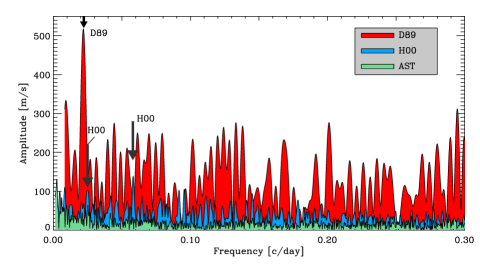
Figure 6.— Residual amplitude spectra of the three radial velocity datasets from ast (black), Hatzes & Cochran (2000; blue), and Dinshaw et al. (1989; red). The low frequency peaks claimed in the previous studies are marked by arrows.

5. Evidence for additional intrinsic variation

In the following we will look at the evidence for variation in Polaris beyond the 4 d main mode. The analysis is based on the ast and wire datasets and data from two previous radial velocity campaigns. The ast dataset is the most accurate at low frequencies, and can be used to look for long periods (Sect. 5.1). The wire dataset consists of three week-long runs with very high precision and can be used to study low-amplitude variation (Sect. 5.2). The noise in the smei dataset is distinctly non-white, as mentioned briefly in Sect. 2. Therefore, we did not use this dataset in the following investigations, except for the subtraction of the 4 d mode, where smei provides the most accurate frequency and phase.

5.1. Long-period variation

In addition to the 4 d mode, a few studies have claimed variation at long periods, e.g. $P=9.75$ d (Kamper et al., 1984), $45.3\pm 0.2$ d Dinshaw et al. (1989), and $40.2\pm 0.7$ d and $17.2$ d (Hatzes & Cochran, 2000). To confirm these claims we reanalysed the original datasets of Dinshaw et al. (1989) and Hatzes & Cochran (2000). The basic properties of these datasets are listed in Table 1.

In Fig. 6 we compare the amplitude spectra of the spectroscopic data from ast, Dinshaw et al. (1989) and Hatzes & Cochran (2000), after subtracting the 4 d period and the long-period trend due to the binary orbit. The ast spectrum was calculated taking the amplitude increase into account (cf. Sect. 4). As a result, the residual double peak seen at $\sim 0.252$ c day^-1 is no longer visible (compare Fig. 6 with the bottom panel in Fig. 3). In the ast amplitude spectrum we see no significant peaks from $0.02$–$0.3$ c day^-1 ($P=3$–$50$ days). We set an upper limit on the amplitude at 100 m s^-1, which is four times the average level in the amplitude spectrum in this frequency interval.

The dataset by Hatzes & Cochran (2000) consists of 42 data points distributed unevenly over 640 days, providing a very complicated spectral window. The dataset comprises very precise radial velocities collected with an iodine cell as a reference (rms residuals are 70 m s^-1). Hatzes & Cochran (2000) detected two peaks with almost equal amplitude at $f_{\rm H00}^{\rm A}=0.0249$ and $f_{\rm H00}^{\rm B}=0.0581$ c day^-1. In the amplitude spectrum in Fig. 6 we find only one of these peaks to be significant ($f_{\rm H00}^{\rm B}=0.05834\pm 0.00014$ c day^-1 with amplitude $A=163\pm 25$ m s^-1). We made 100 simulations of the data including this frequency, white noise, and a $1/f$ noise component consistent with the observations. The inserted $f_{\rm H00}^{\rm B}$ frequency was only recovered in 49 of the 100 simulations. Interestingly, in the other simulations the highest peaks were clustered close to $f_{\rm H00}^{\rm A}$ ($0.025\pm 0.007$ c day^-1 with amplitude $A=167\pm 22$ m s^-1), indicating that the two peaks detected by Hatzes & Cochran (2000) are due to the complicated spectral window.

The dataset by Dinshaw et al. (1989) comprises 175 velocities distributed over 241 days. The precision is 440 m s^-1, as estimated from the rms of the residuals after subtracting the 4 d mode. In addition to this mode we detect a peak at $1.02199\pm 0.00024$ c day^-1 with strong aliases at $\pm 1$ c day^-1. Dinshaw et al. (1989) found one of the alias peaks ($f_{\rm D89}=0.0221\pm 0.0001$ c day^-1) to be the highest and suggested that it was intrinsic to Polaris. We measure the amplitude to be $A=0.542\pm 0.067$ km s^-1, but such a strong signal is not seen in the more recent dataset by Hatzes & Cochran (2000) or in any of our datasets (see Figs. 3 and 6). For these reasons we believe that this peak is a 1 c day^-1 artifact, likely caused by instrumental drift in combination with the spectral window.

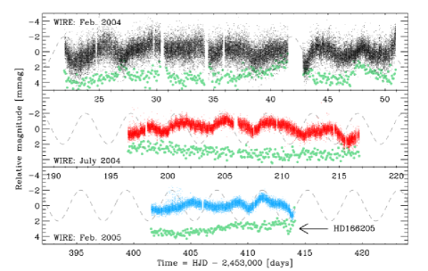
Figure 7.— Residuals in the three wire light curves of Polaris and the comparison star HD 166205 (large $\bullet$ symbols offset by 3 mmag). The dashed curve is a sinusoid with the 4 d period and an amplitude set arbitrarily to 2 mmag.

5.2. Low-amplitude variation

The residuals in the wire light curves, after having subtracted the 4 d period, are shown in Fig. 7. The drifts seen in the wire light curves correspond to periods from 2–6 d, i.e. similar to the 4 d main mode. Before interpreting this variation, it is important to investigate if these variations are due to improper subtraction of the main period or due to instrumental drift.

To test the first caveat, we compared the residuals when subtracting the fit to the smei data and when subtracting fits to the individual wire datasets. We find that the residuals are quite similar, and the conclusions reached here are not affected by the adopted approach. In the following, we have used the most accurate value for the frequency and phase, which is from the fit of the main mode to the smei data, while we used the amplitudes fitted to the individual wire datasets.

The second caveat is instrumental drift and we tested this by using a comparison star. During the observations with the wire star tracker four other stars were monitored on the same CCD. However, not all are suited as comparison stars: HD 5848 is a bright ($V=4.3$) K giant star clearly showing solar-like oscillations (Stello et al., 2008). HD 51802 and HD 174878 are faint ($V=5.1$ and $6.6$) M giants showing variation with long periods. The only suitable comparison star is the A1 V star HD 166205 ($\delta$ UMi; $V=4.4$). In Fig. 7 we also show the light curve of this star with large $\bullet$ symbols. The star is two magnitudes fainter than Polaris, so we binned the data collected within each orbit ($P_{\rm orbit}\simeq 93$ min) to be able to see any low-amplitude variation.

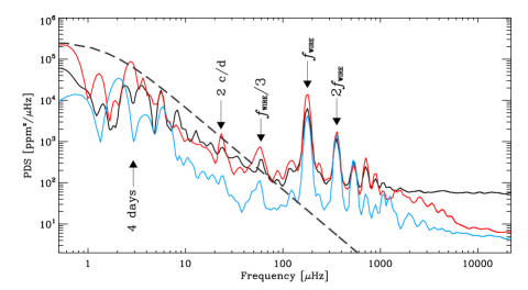
Figure 8.— Power density spectrum (PDS) of the residual light curves from wire shown in Fig. 7. The dashed line is a scaling of the granulation measured in the Sun. The arrows mark the 4 d main period and frequencies that are due to the wire orbit.

The clear variation in the residuals of the wire photometry is not seen in the hot comparison star HD 166205. The fact that it is seen in three light curves obtained with wire at three different epochs spanning one year gives us some confidence that the signal is intrinsic to Polaris. We will discuss two possible explanations for the observed variation here, namely granulation and star spots.

To investigate in detail how the variation in the wire light curves depends on frequency, we show their power density spectra (PDS) in Fig. 8 in a logarithmic plot. The virtue of the PDS is that one can directly compare the properties of datasets, which have different temporal coverage and noise characteristics. Each PDS shows a clear increase from the white noise level around $10$ mHz towards low frequencies. The arrows mark the harmonics of the orbital frequency of wire ($f_{\rm WIRE}=178$ $\mu$Hz), one third of the wire orbital frequency, and 2 c/day. These frequencies are observed in almost all wire datasets, and are due to a combination of a low duty cycle (typically 20–40%) and scattered light from earth shine. Also marked is the location of the 4 d mode ($f=2.91$ $\mu$Hz), which has been subtracted.

To see if granulation could explain the increase in the PDS towards low frequencies, we have used a scaling of the granulation observed in the Sun. This is based on virgo satellite observations of the Sun-as-a-star, and the scaling is done both in terms of amplitude and timescale, following Kjeldsen & Bedding (in preparation; see also Stello et al. 2007). This prediction is shown as the dashed line in Fig. 8. This is a scaling over three orders of magnitude in luminosity from the Sun to the super giant Polaris, so it is intriguing that the prediction of the granulation signal agrees with the observations within a factor of $3.0\pm 0.5$ in amplitude.

Both Dinshaw et al. (1989) and Hatzes & Cochran (2000) discussed evidence for star spots on Polaris. We argue that this is not the cause of the observed variation in the wire data, since the time-scale is only a few days. That would imply very rapid rotation, which is unlikely for such an evolved star.

6. Discussion and conclusion

From $4.5$ years of intensive monitoring of Polaris we find that the amplitude of the 4-day main mode has increased steadily by about 30% in both radial velocity and flux amplitude. The rate of increase in the amplitude from 2003–2007 is slightly steeper than the decrease from the fit by Kamper & Fernie (1998) for the period 1980–1994. Other sources have also found a recent increase in the amplitude of Polaris (Engle et al. 2004; Turner 2007, private communication).

The result that the amplitude of Polaris is now increasing has implications for earlier explanations of the change in amplitude as a cessation of pulsation due to the Cepheid’s evolution towards the edge of the instability strip. At the very least, whatever the process is, it is not a simple monotonic progression through the HR diagram, unless this stage of evolution is more complex than previously thought. The recovery of the amplitude suggests that the phenomenon is cyclic. As such, it is likely to be associated in some way with pulsation rather than with evolution.

A possible explanation for the increase in amplitude could be the beating of two closely spaced modes (Breger & Kolenberg, 2006). To exhibit a beat period as long as the amplitude variation of Polaris (likely a few 100 years), the modes would have to be very closely spaced indeed. Among classical Cepheids, amplitude variation is extremely uncommon. The only case where it is firmly established is in V 473 Lyrae (Burki et al., 1986), where the variation occurs over only a few years. In RR Lyrae stars, the Blazhko effect is well known, and thought to be the result of mode beating, although it is not completely understood. Since the amplitude changes in Polaris are well established, they require further observations and consideration theoretically to unravel the cause.

There are other interesting aspects to the main oscillation mode. The characterization of the period change is puzzling since analysis of $O-C$ diagrams spanning more than a century reveal that the period change is not linear. There may have been a “glitch” in both the period change and the amplitude in the mid-1960’s (Turner et al., 2005), rather than smooth changes. We measured 239 epochs of maximum light but the time span of the observations of $4.5$ years is too short to investigate the period change. This is another aspect of the pulsation that demands further observation.

A few radial velocity campaigns have claimed the presence of additional long-period variation in Polaris. We have analysed the original datasets by Dinshaw et al. (1989) and Hatzes & Cochran (2000) and we conclude that these long periods are likely spurious detections caused by instrumental drifts (Dinshaw et al., 1989) or insufficient data leading to a complicated spectral window (Hatzes & Cochran, 2000). From our 3.8 yr of monitoring with ast, we set an upper limit on the variation in radial velocity at 100 m s^-1 for periods in the range 3–50 d (except for the 4 d main mode).

In the wire data we find evidence of low-amplitude variation (peak-to-peak $2$ mmag) at time scales of 2–6 days, which are likely intrinsic to Polaris. We applied a simple scaling of observed solar values for the characteristic timescale and amplitude of the granulation. Although this is a scaling over three orders of magnitude in luminosity, the prediction agrees with the observed variation in Polaris within a factor $3.0\pm 0.5$. Thus, we conclude that the variation in the wire data could be due to granulation.

References

- Arellano Ferro (1983) Arellano Ferro, A. 1983, ApJ, 274, 755
- Breger & Kolenberg (2006) Breger, M., & Kolenberg, K. 2006, A&A, 460, 167
- Bruntt (2007) Bruntt, H. 2007, Communications in Asteroseismology, 150, 326
- Bruntt et al. (2005) Bruntt, H., Kjeldsen, H., Buzasi, D. L., & Bedding, T. R. 2005, ApJ, 633, 440
- Bruntt et al. (2007) Bruntt, H., Stello, D., Suárez, J. C., Arentoft, T., Bedding, T. R., Bouzid, M. Y., Csubry, Z., Dall, T. H., Dind, Z. E., Frandsen, S., Gilliland, R. L., Jacob, A. P., Jensen, H. R., Kang, Y. B., Kim, S.-L., Kiss, L. L., Kjeldsen, H., Koo, J.-R., Lee, J.-A., Lee, C.-U., Nuspl, J., Sterken, C., & Szabó, R. 2007, MNRAS, 378, 1371
- Burki et al. (1986) Burki, G., Schmidt, E. G., Arellano Ferro, A., Fernie, J. D., Sasselov, D., Simon, N. R., Percy, J. R., & Szabados, L. 1986, A&A, 168, 139
- Dinshaw et al. (1989) Dinshaw, N., Matthews, J. M., Walker, G. A. H., & Hill, G. M. 1989, AJ, 98, 2249
- Eaton & Williamson (2004) Eaton, J. A., & Williamson, M. H. 2004, Astronomische Nachrichten, 325, 522
- Eaton & Williamson (2007) —. 2007, PASP, submitted
- Engle et al. (2004) Engle, S. G., Guinan, E. F., & Koch, R. H. 2004, in Bulletin of the American Astronomical Society, Vol. 36, 744
- Evans et al. (2002) Evans, N. R., Sasselov, D. D., & Short, C. I. 2002, ApJ, 567, 1121
- Eyles et al. (2003) Eyles, C. J., Simnett, G. M., Cooke, M. P., Jackson, B. V., Buffington, A., Hick, P. P., Waltham, N. R., King, J. M., Anderson, P. A., & Holladay, P. E. 2003, Sol. Phys., 217, 319
- Feast & Catchpole (1997) Feast, M. W., & Catchpole, R. M. 1997, MNRAS, 286, L1
- Fernie et al. (1993) Fernie, J. D., Kamper, K. W., & Seager, S. 1993, ApJ, 416, 820
- Hatzes & Cochran (2000) Hatzes, A. P., & Cochran, W. D. 2000, AJ, 120, 979
- Jackson et al. (2004) Jackson, B. V., Buffington, A., Hick, P. P., Altrock, R. C., Figueroa, S., Holladay, P. E., Johnston, J. C., Kahler, S. W., Mozer, J. B., Price, S., Radick, R. R., Sagalyn, R., Sinclair, D., Simnett, G. M., Eyles, C. J., Cooke, M. P., Tappin, S. J., Kuchar, T., Mizuno, D., Webb, D. F., Anderson, P. A., Keil, S. L., Gold, R. E., & Waltham, N. R. 2004, Sol. Phys., 225, 177
- Kamper (1996) Kamper, K. W. 1996, JRASC, 90, 140
- Kamper et al. (1984) Kamper, K. W., Evans, N. R., & Lyons, R. W. 1984, JRASC, 78, 173
- Kamper & Fernie (1998) Kamper, K. W., & Fernie, J. D. 1998, AJ, 116, 936
- Montgomery & O’Donoghue (1999) Montgomery, M. H., & O’Donoghue, D. 1999, Delta Scuti Star Newsletter, 13, 28
- Moskalik & Ogłoza (2000) Moskalik, P., & Ogłoza, W. 2000, in Astronomical Society of the Pacific Conference Series, Vol. 203, IAU Colloq. 176: The Impact of Large-Scale Surveys on Pulsating Star Research, ed. L. Szabados & D. Kurtz, 237–238
- Parenago (1956) Parenago, P. P. 1956, Peremennye Zvezdy, 11, 236
- Stello et al. (2007) Stello, D., Bruntt, H., Kjeldsen, H., Bedding, T. R., Arentoft, T., Gilliland, R. L., Nuspl, J., Kim, S.-L., Kang, Y. B., Koo, J.-R., Lee, J.-A., Sterken, C., Lee, C.-U., Jensen, H. R., Jacob, A. P., Szabó, R., Frandsen, S., Csubry, Z., Dind, Z. E., Bouzid, M. Y., Dall, T. H., & Kiss, L. L. 2007, MNRAS, 377, 584
- Stello et al. (2008) Stello, D., Bruntt, H., Preston, H., & Buzasi, D. 2008, ApJ, 674, L53
- Szabados (1977) Szabados, L. 1977, Mitt. Sternw. Ungarisch. Akad. Wiss., Budapest-Szabadsághegy, 70, 1
- Tarrant et al. (2007) Tarrant, N. J., Chaplin, W. J., Elsworth, Y., Spreckley, S. A., & Stevens, I. R. 2007, MNRAS, 382, L48
- Turner et al. (2005) Turner, D. G., Savoy, J., Derrah, J., Abdel-Sabour Abdel-Latif, M., & Berdnikov, L. N. 2005, PASP, 117, 207
- van Leeuwen et al. (2007) van Leeuwen, F., Feast, M. W., Whitelock, P. A., & Laney, C. D. 2007, MNRAS, 379, 723