Order-Reducing Form Symmetries and Semiconjugate

Factorizations of Difference Equations

H. SEDAGHAT

Abstract. The scalar difference equation $x_{n+1}=f_{n}(x_{n},x_{n-1},\cdots,x_{n-k})$ may exhibit symmetries in its form that allow for reduction of order through substitution or a change of variables. Such form symmetries can be defined generally using the semiconjugate relation on a group which yields a reduction of order through the semiconjugate factorization of the difference equation of order ${\small k+1}$ into equations of lesser orders. Different classes of equations are considered including separable equations and homogeneous equations of degree 1. Applications include giving a complete factorization of the linear non-homogeneous difference equation of order ${\small k+1}$ into a system of ${\small k+1}$ first order linear non-homogeneous equations in which the coefficients are the eigenvalues of the higher order equation. Form symmetries are also used to explain the complicated multistable behavior of a separable, second order exponential equation.

Keywords. Form symmetry, order reduction, semiconjugate, groups, difference equations, linear non-homogeneous, separable, homogeneous of degree 1, multistability

1 Introduction

Certain difference equations have symmetries in their expressions that allow a reduction of their orders through substitutions of new variables. For instance, consider the second order, scalar difference equation

$$x_{n+1}=x_{n}+g_{n}(x_{n}-x_{n-1})$$ (1)

where $g_{n}$ is a real function for each integer $n$. This equation has a symmetry in its form that is easy to identify when (1) is re-written as

$$x_{n+1}-x_{n}=g_{n}(x_{n}-x_{n-1}).$$ (2)

Now, setting $t_{n}=x_{n}-x_{n-1}$ changes Eq.(2) to the first order equation

$$t_{n+1}=g_{n}(t_{n}).$$ (3)

The expression $x_{n}-x_{n-1}$ is an example of what we may call a form symmetry. Substituting a new variable $t_{n}$ for this form symmetry in (2) gave the lower order equation (3). The form symmetry also establishes a link between the second order equation and the first order one, in the sense that information about each solution $\{t_{n}\}$ of (3) can then be translated into information about the corresponding solution of (1) using the equation

$$x_{n}=x_{n-1}+t_{n}=x_{0}+\sum_{k=1}^{n}t_{k}$$ (4)

where $x_{0}$ is an initial value for (1). Along similar lines, the non-homogeneous linear difference equation

$$x_{n+1}+px_{n}+qx_{n-1}=\alpha_{n}\quad\text{with }1+p+q=0$$ (5)

has at least two form symmetries. First, setting $p=-1-q$ and rearranging terms in (5) reveals the form symmetry $x_{n}-x_{n-1}$ and the corresponding order-reducing substitution:

$$x_{n+1}-x_{n}=\alpha_{n}+q(x_{n}-x_{n-1})\Rightarrow t_{n+1}=\alpha_{n}+qt_{n}.$$ (6)

Further,

$$x_{n+1}-qx_{n}=\alpha_{n}-(p+q)x_{n}-qx_{n-1}=\alpha_{n}+x_{n}-qx_{n-1}\Rightarrow t_{n+1}=\alpha_{n}+t_{n}.$$ (7)

Thus $x_{n}-qx_{n-1}$ is also a form symmetry of (5). Note that the coefficients $q$ and $1$ of $t_{n}$ in (6) and (7), respectively, are both eigenvalues of the homogeneous part of (5), i.e., roots of the characteristic polynomial $z^{2}+pz+q$ when $p+q=-1$. Later in this article we show that this relationship holds for all linear difference equations.

These and many other types of known form symmetries of difference equations of type

$$x_{n+1}=f_{n}(x_{n},x_{n-1},\cdots,x_{n-k}).$$ (8)

can be defined in terms of semiconjugacy; in [22] there is a basic discussion of this topic for real functions but we give a more general definition in this article. The idea of reducing order via semiconjugacy is basically simple; we find functions that are semiconjugate to the given functions $f_{n}$ but which have fewer variables than $k+1,$ i.e., the order of (8). Then the semiconjugate relation simultaneously determines both a form symmetry and a factorization of Eq.(8). This factorization of difference equations, which is also a formal representation of the substitution process discussed above, yields a pair of lower order equations. This pair is made up of a factor equation such as (3) and an associated equation such as (4) that is derived from the form symmetry and relates the factor equation to the original one. The orders of the factor equation and the associated one always add up to the order of the original scalar equation.

The aim of this article is to formalize, within the framework of semiconjugacy, the concept of form symmetry and its use in reduction of order by substitutions. In addition to unifying various ad hoc techniques, this approach also gives rise to new methods for analyzing higher order difference equations. Some of these new methods are described in this article along with examples and applications.

Symmetries of a different kind have already been used to study higher order difference equations or systems of first order ones. A well-known approach involves adaptation of the Lie symmetry concept from differential equations to difference equations; see, e.g., [9] for a general discussion of the discrete case covering various topics such as reduction of order, integrability and finding explicit solutions. Also see [4], [13], [15] for additional ideas and techniques. The main difference between the concepts of form symmetry and Lie symmetry may be summed up as follows: Form symmetries are sought in the difference equation itself whereas Lie symmetries exist in the solutions of the equation. The existence of either type of symmetry can yield valuable information about the dynamics and the solutions of the difference equation with a variety of applications such as reduction of order.

2 Semiconjugate forms

The material in this section substantially extends the notions in [22] to the more general group context. For related results and background material on difference equations see, e.g., [1], [3], [5], [8], [12].

In this article, $G$ denotes a non-trivial group. The group structure provides a suitable framework for our results. However, in most applications $G$ turns out to be a substructure of a more complex object such as a vector space, a ring or an algebra possessing a compatible or natural metric topology. In typical studies involving difference equations and discrete dynamical systems, $G$ is a group of real or complex numbers. We may define each mapping $f_{n}$ on the ambient sturcture as long as the following invariance condition holds

$$f_{n}(G^{k+1})\subset G\text{ \ for all }n.$$ (9)

If (9) holds then for each set of initial values $x_{0},x_{-1},\ldots,x_{-k}$ in $G$ Eq.(8) recursively generates a solution or orbit $\{x_{n}\}_{n=-1}^{\infty}$ in $G.$ Before defing form symmetries for (8), it is necessary to discuss some general defintions involving systems.

Let $1\leq m\leq k.$ We say that a self map $F_{n}=[f_{1,n},\ldots,f_{k+1,n}]$ of $G^{k+1}$ is semiconjugate to a self map $\Phi_{n}$ of $G^{m}$ if there is a function $H:G^{k+1}\rightarrow G^{m}$ such that for every $n,$

$$H\circ F_{n}=\Phi_{n}\circ H.$$ (10)

Each mapping $\Phi_{n}$ is called a semiconjugate factor of the corresponding $F_{n}$. Suppose that

$$H(u_{0},\ldots,u_{k}) =[h_{1}(u_{0},\ldots,u_{k}),\ldots,h_{m}(u_{0},\ldots,u_{k})]$$

$$\Phi_{n}(t_{1},\ldots,t_{m}) =[\phi_{1,n}(t_{1},\ldots,t_{m}),\ldots,\phi_{m,n}(t_{1},\ldots,t_{m})]$$

where $h_{j}:G^{k+1}\rightarrow G$ and $\phi_{j,n}:G^{m}\rightarrow G$ are the corresponding component functions. Then identity (10) is equivalent to the system

$$h_{j}(f_{1,n}(u_{0},\ldots,u_{k}),\ldots,f_{k+1,n}(u_{0},\ldots,u_{k})) =\phi_{j,n}(h_{1}(u_{0},\ldots,u_{k}),\ldots,h_{m}(u_{0},\ldots,u_{k}))$$

$$j =1,2,\ldots,m.$$ (11)

If the functions $f_{j,n}$ are given then (11) is a system of functional equations whose solutions $h_{j},\phi_{j,n}$ give the maps $H$ and $\Phi_{n}.$ The functions $\Phi_{n}$ on $G^{m}$ define a system with lower dimension than that defined by the functions $F_{n}$ on $G^{k+1}.$ For a given solution $\{X_{n}\}$ of the equation

$$X_{n+1}=F_{n}(X_{n}),\quad X_{0}\in G^{k+1}$$ (12)

let $Y_{n}=H(X_{n})$ for $n=0,1,2,\ldots$ Then

$$Y_{n+1}=H(X_{n+1})=H(F_{n}(X_{n}))=\Phi_{n}(H(X_{n}))=\Phi_{n}(Y_{n})$$

so that $\{Y_{n}\}$ satisfies the lower order equation

$$Y_{n+1}=\Phi_{n}(Y_{n}),\quad Y_{0}=H(X_{0})\in G^{m}.$$ (13)

The relationship between the solutions of (12) and those of (13) is not generally straightforward; however, information about the solutions of (13) can shed light on the dynamics of (12). The case where $G=\mathbb{R}$, $m=1$ and $F_{n}=F$ is time-independent (or autonomous) is of some interest because in this case Eq.(13) is a first order difference equation on the real numbers and as such its dynamics are much better understood than that of the higher dimensional Eq.(12). This case is discussed in detail in [22].

3 Order-reducing form symmetries

For the scalar difference equation (8) that is of interest in this article, each $F_{n}$ is the associated vector map (or unfolding) of the function $f_{n}$ in Eq.(8), i.e.,

$$F_{n}(u_{0},\ldots,u_{k})=[f_{n}(u_{0},\ldots,u_{k}),u_{0},\ldots,u_{k-1}].$$

Even if each such $F_{n}$ is semiconjugate to an $m$-dimensional map $\Phi_{n}$ as in (10), the preceding discussion only gives the system (13) in which the maps $\Phi_{n}$ are not necessarily of scalar type similar to $F_{n}.$ While this may be unavoidable in some cases, adding a few reasonable restrictions can ensure that each $\Phi_{n}$ is also of scalar type. To this end, define

$$h_{1}(u_{0},\ldots,u_{k})=u_{0}\ast h(u_{1},\ldots,u_{k})$$ (14)

where $h:G^{k}\rightarrow G$ is a function to be determined and $\ast$ denotes the group operation. This restriction on $H$ makes sense for Eq.(8), which is of recursive type; i.e., $x_{n+1}$ given explicitly by functions $f_{n}$. With these restrictions on $H$ and $F_{n}$ the first equation in (11) is given by

$$f_{n}(u_{0},\ldots,u_{k})\ast h(u_{0},\ldots,u_{k-1})=g_{n}(u_{0}\ast h(u_{1},\ldots,u_{k}),\ldots,h_{m}(u_{0},\ldots,u_{k}))$$ (15)

where for notational convenience we have set

$$g_{n}\doteq\phi_{1,n}:G^{m}\rightarrow G.$$

Eq.(15) is a functional equation in which the functions $h,h_{j},g_{n}$ may be determined in terms of the given functions $f_{n}$. Our aim is ultimately to extract a scalar equation of order $m$ such as

$$t_{n+1}=g_{n}(t_{n},\ldots,t_{n-m+1})$$ (16)

from (15) in such a way that the maps $\Phi_{n}$ will be of scalar type. The basic framework is already in place; let $\{x_{n}\}$ be a solution of Eq.(8) and define

$$t_{n}=x_{n}\ast h(x_{n-1},\ldots,x_{n-k}).$$

Then the left hand side of (15) is

$$x_{n+1}\ast h(x_{n},\ldots,x_{n-k+1})=t_{n+1}.$$

which gives the initial part of the difference equation (16). In order that the right hand side of (15) coincide with that in (16) it is necessary to define

$$h_{j}(x_{n},\ldots,x_{n-k})=t_{n-j+1}=x_{n-j+1}\ast h(x_{n-j},\ldots,x_{n-k-j+1}),\quad j=2,\ldots,m.$$ (17)

Since the left hand side of (17) does not depend on terms $x_{n-k-1},\ldots,x_{n-k-j+1}$ it follows that the function $h_{j}$ must be constant in its last few coordinates. Since $h$ deos not depend on $j$ the number of constant coordinates is found from the last function $h_{m}.$ Specifically, we have

$$h_{m}(x_{n},\ldots,x_{n-k})=x_{n-m+1}\ast h(\underset{k-m+1\text{ variables}}{\underbrace{x_{n-m},\ldots,x_{n-k}}},\underset{m-1\text{ terms with }h\text{ constant}}{\underbrace{x_{n-k-1},\ldots,x_{n-k-m+1}}})$$ (18)

The preceding condition leads to the necessary restrictions on $h$ and every $h_{j}$ for a consistent derivation of (16) from (15), so (18) is a consistency condition. Now from (17) and (18) we obtain for $(u_{0},\ldots,u_{k})\in G^{k+1}$

$$h_{j}(u_{0},\ldots,u_{k})=u_{j-1}\ast h(u_{j},u_{j+1}\ldots,u_{j+k-m}),\quad j=1,\ldots,m.$$ (19)

We refer to $H=[h_{1},\ldots,h_{m}]$ as a form symmetry for Eq.(8) if the components $h_{j}$ are defined by (19). Since the range of $H$ has a lower dimension than its domain, we say that $H$ is an order-reducing form symmetry.

Using the forms in (19) for $h_{j}$ in (15) for every solution $\{x_{n}\}$ of Eq.(8) we obtain the following pair of equations from (15), the first of which is just (16):

$$t_{n+1} =g_{n}(t_{n},\ldots,t_{n-m+1}),$$ (20a)

$$x_{n+1} =t_{n+1}\ast h(x_{n},\ldots,x_{n-k+m})^{-1}.$$ (20b)

The power $-1$ represents group inversion in $G.$ The first equation (20a) may be called a factor of Eq.(8) since it is distilled from the semiconjugate factor $\Phi_{n}.$ The second equation (20b) that links the factor to the original equation may be called a cofactor of Eq.(8). We call the system of equations (20) a semiconjugate (SC) factorization of Eq.(8).

Note that if $\{t_{n}\}$ is a given solution of (20a) then using this sequence in (20b) produces a solution $\{x_{n}\}$ of (8). Conversely, if $\{x_{n}\}$ is a solution of (8) then the sequence $t_{n}=x_{n}\ast h(x_{n-1},\ldots,x_{n-k+m-1})$ is a solution of (20a) with initial values

$$t_{-j}=x_{-j}\ast h(x_{-j-1},\ldots,x_{-j-k+m-1}),\quad j=0,\ldots,m-1.$$

Since solutions of the pair of equations (20a) and (20b) coincide with the solutions of the scalar equation (8), we say that the pair (20a) and (20b) is equivalent to (8). The following summarizes the preceding discussions.

Theorem 1. Let $k\geq 1$, $1\leq m\leq k$ and suppose that there are functions $h:G^{k-m+1}\rightarrow G$ and $g_{n}:G^{m}\rightarrow G$ that satisfy equations (15) and (19). Then with the order-reducing form symmetry

$$H(u_{0},\ldots,u_{k})=[u_{0}\ast h(u_{1},\ldots,u_{k+1-m}),\ldots,u_{m-1}\ast h(u_{m},\ldots,u_{k})]$$

Eq.(8) is equivalent to the SC factorization consisting of the pair of equations (20a) and (20b) whose orders $m$ and $k+1-m$ respectively, add up to the order of (8).

In this setting we say that the SC factorization (20) gives a type-($m,k+1-m$) order reduction for Eq.(8), or that (8) is a type-($m,k+1-m$) equation. A second order difference equation ($k=1$) can have only the order-reduction type (1,1) into two first order equations although the factor and cofactor equations are not uniquely defined. In general, a higher order difference equation may have more than one SC factorization. A third order equation can have two order-reduction types, namely, (1,2) and (2,1). Of the $k$ possible order reduction types for an equation of order $k+1$ the two extreme ones, namely, $(1,k)$ and $(k,1)$ have the extra appeal of having an equation of order 1 as either a factor or a cofactor. In the next two sections we discuss classes of higher order difference equations having one of these order-reduction types.

We note that the SC factorization of Theorem 1 does not require the determination of $\phi_{j,n}$ for $j\geq 2.$ For completeness, we close this section by showing that each coordinate function $\phi_{j,n}$ projects into coordinate $j-1$ for $j>1,$ thus showing that $\Phi_{n}$ is of scalar type, i.e., it is the unfolding of Eq.(16) in the same sense that $F_{n}$ unfolds (8). If the maps $h_{j}$ are given by (19) then for $j\geq 2$ (11) gives

$$\phi_{j,n}(h_{1}(u_{0},\ldots,u_{k}),\ldots,h_{m}(u_{0},\ldots,u_{k})) =h_{j}(f_{n}(u_{0},\ldots,u_{k}),u_{0},\ldots,u_{k-1})$$

$$=u_{j-2}\ast h(u_{j-1},u_{j}\ldots,u_{j+k-m-1})$$

$$=h_{j-1}(u_{0},\ldots,u_{k}).$$

Therefore, for each $n$ and for every $(t_{1},\ldots,t_{m})\in H(G^{k+1})$ we have

$$\Phi_{n}(t_{1},\ldots,t_{m})=[g_{n}(t_{1},\ldots,t_{m}),t_{1},\ldots,t_{m-1}]$$

i.e., $\Phi_{n}|_{H(G^{k+1})}$ is of scalar type. Further, if $H$ is defined component-wise by (19) then $H(G^{k+1})=G^{m};$ i.e., $H$ is onto $G^{m}$ so that $\Phi_{n}$ is of scalar type. To prove the onto claim, we pick arbitrary $[t_{1},\ldots,t_{m}]\in G^{m}$ and set $u_{m-1}=t_{m}\ast h(u_{m},u_{m+1}\ldots,u_{k})^{-1}$ where $u_{m}=u_{m+1}=\ldots u_{k}=1$ (the group identity). Then

$$t_{m} =u_{m-1}\ast h(1,1\ldots,1)$$

$$=u_{m-1}\ast h(u_{m},u_{m+1}\ldots,u_{k})$$

$$=h_{m}(u_{0},\ldots,u_{k})$$

$$=h_{m}(u_{0},\ldots,u_{m-2},t_{m}\ast h(1,1\ldots,1)^{-1},1\ldots,1).$$

for any choice of $u_{0},\ldots,u_{m-2}\in G.$ Similarly, define $u_{m-2}=t_{m-1}\ast h(u_{m-1},u_{m}\ldots,u_{k-1})^{-1}$ so as to get

$$t_{m-1} =u_{m-2}\ast h(u_{m-1},u_{m}\ldots,u_{k-1})$$

$$=h_{m-1}(u_{0},\ldots,u_{k})$$

$$=h_{m-1}(u_{0},\ldots,u_{m-3},t_{m-1}\ast h(u_{m-1},1\ldots,1)^{-1},u_{m-1},1\ldots,1)$$

for any choice of $u_{0},\ldots,u_{m-3}\in G.$ Continuing in this way, induction leads to selection of $u_{m-1},\ldots,u_{0}$ such that

$$t_{j}=h_{j}(u_{0},\ldots,u_{m-1},1,\ldots,1),\quad j=1,\ldots,m$$

and it is proved that $H$ is onto $G^{m}.$

4 HD1 and other type-$(k,1)$ factorizations

If $m=k$ then the function $h:G\rightarrow G$ in (19) is of one variable and we obtain a type-$(k,1)$ order reduction with form symmetry

$$H(u_{0},\ldots,u_{k})=[u_{0}\ast h(u_{1}),u_{1}\ast h(u_{2})\ldots,u_{k-1}\ast h(u_{k})]$$ (21)

and SC factorization

$$t_{n+1} =g_{n}(t_{n},t_{n-1},\ldots,t_{n-k+1})$$

$$x_{n+1} =t_{n+1}\ast h(x_{n})^{-1}$$

where the functions $g_{n}:G^{k}\rightarrow G$ are determined by the given functions $f_{n}$ in (8) as in the previous section.

The simplest example of a non-constant $h$ in this setting is the identity function $h(u)=u$ for all $u\in G.$ An example of a type-$(k,1)$ difference equation having this type of form symmetry over $(0,\infty)$ under ordinary multiplication is the rational equation

$$x_{n+1}=\frac{ax_{n-1}}{x_{n}x_{n-1}+b},\quad a,b>0.$$ (22)

The term $x_{n}x_{n-1}$ in the denominator suggests multiplying (22) by $x_{n}$ on both sides and substituting

$$t_{n}=x_{n}x_{n-1}=x_{n}h(x_{n-1})$$

to get the SC factorization

$$t_{n+1} =\frac{at_{n}}{t_{n}+b}=g(t_{n}),\quad t_{0}=x_{0}x_{-1}$$ (23)

$$x_{n+1} =\frac{t_{n+1}}{x_{n}}=\frac{t_{n+1}}{h(x_{n})}.$$

Further, Eq.(23) can be made linear by the change of variables $s_{n}=1/t_{n}.$ For an exhaustive treatment of (22) based on these ideas, see [16]. Another form symmetry of type (21) that is defined on $\mathbb{C}$ or $\mathbb{R}$ is based on $h(u)=cu$ where $c$ is a fixed, nonzero complex or real number. This type of form symmetry (with real $c$) has been used in e.g., [7] and [17].

In the case where $h(u)=u^{-1}$ is based on group inversion, it is possible to identify the class of functions $f_{n}$ that have the form symmetry (21). Equation (8) is said to be homogeneous of degree 1 (HD1) if for every $n=1,2,3,\ldots$ the functions $f_{n}$ are homogeneous of degree 1 relative to the group $G,$ i.e.,

$$f_{n}(u_{0}\ast t,\ldots,u_{k}\ast t)=f_{n}(u_{0},\ldots,u_{k})\ast t\text{ for all }t,u_{i}\in G,\ i=0,\ldots,k,\ n\geq 1.$$

If $G$ is non-commutative then this definition gives a “right version” of the HD1 property; a “left version” can be defined analogously. We note that the two equations (1) and (5) in the Introduction are HD1 relative to the additive group of real numbers. For comments on homogeneous functions and their abundance on groups we refer to [20]; though stated for functions of two variables, the results in [20] easily extend to any number of variables. The following result shows that the HD1 property characterizes the inversion-based form symmetry and yields a type-$(k,1)$ order-reduction in every case.

Theorem 2. Eq.(8) has the inversion-based form symmetry

$$H(u_{0},\ldots,u_{k})=[u_{0}\ast u_{1}^{-1},\ldots,u_{k-1}\ast u_{k}^{-1}],\quad h(t)=t^{-1}$$ (24)

if and only if $f_{n}$ is HD1 relative to $G$ for all $n$. In this case, (8) has a type-($k,1$) order-reduction with the SC factorization

$$t_{n+1} =f_{n}(1,t_{n}^{-1},(t_{n}\ast t_{n-1})^{-1},\ldots,(t_{n}\ast t_{n-1}\ast\cdots\ast t_{n-k+1})^{-1})$$ (25a)

$$x_{n+1} =t_{n+1}\ast x_{n}.$$ (25b)

Note that the factor difference equation (25a) has order $k$ and its cofactor (25b) is linear non-autonomous of order one in $x_{n}$.

Proof. First, assume that (8) has the form symmetry (24) that satisfies Eq.(15) for given functions $g_{n},$ i.e.,

$$f_{n}(u_{0},\ldots,u_{k})\ast u_{0}^{-1}=g_{n}(u_{0}\ast u_{1}^{-1},\ldots,u_{k-1}\ast u_{k}^{-1}).$$ (26)

Let $t\in G$ be arbitrary. Then for all $n$ (26) implies

$$f_{n}(u_{0}\ast t,\ldots,u_{k}\ast t) =g_{n}((u_{0}\ast t)\ast(u_{1}\ast t)^{-1},\ldots,(u_{k-1}\ast t)\ast(u_{k}\ast t)^{-1})\ast(u_{0}\ast t)$$

$$=[g_{n}(u_{0}\ast u_{1}^{-1},\ldots,u_{k-1}\ast u_{k}^{-1})\ast u_{0}]\ast t$$

$$=f_{n}(u_{0},\ldots,u_{k})\ast t.$$

It follows that $f_{n}$ is HD1 relative to $G$ for all $n$ and the first part of the theorem is proved. The converse is proved in a straightforward fashion; see [21].

Remarks.

1. Equation (25b) can be solved explicitly in terms of a solution $\{t_{n}\}$ of (25a) as follows:

$$x_{n}={\textstyle\prod_{i=0}^{n-1}}t_{n-i}\ast x_{0}\quad n=1,2,3,\ldots$$ (27)

where the multiplicative notation is used for iterations of the group opreation $\ast.$ In additive (and commutative) notation, (27) takes the form

$$x_{n}=x_{0}+{\textstyle\sum_{i=1}^{n}}t_{i}.$$ (28)

2. We can quickly construct Eq.(25a) directly from (8) in the HD1 case by making the substitutions

$$1\rightarrow x_{n},\quad(t_{n}t_{n-1}\cdots t_{n-i+1})^{-1}\rightarrow x_{n-i}\ \ \text{for }i=1,2,\ldots,k.$$ (29)

Recall that 1 represents the group identity in multiplicative notation. In additive notation (29) takes the form

$$0\rightarrow x_{n},\quad-t_{n}-t_{n-1}\cdots-t_{n-i+1}\rightarrow x_{n-i}\ \ \text{for }i=1,2,\ldots,k.$$ (30)

Previous studies involving HD1 equations implicitly use the idea behind Theorem 2 above to reduce second order equations to first order ones; see e.g. [6], [10], [16]. Examples 1-3 next illustrate Theorem 2 and some associated concepts.

Example 1. Consider the rational delay difference equation

$$x_{n+1}=x_{n}\left(\frac{a_{n}x_{n-k+1}}{x_{n-k}}+b_{n}\right),\quad x_{0},x_{-1},\ldots,x_{-k}>0$$ (31)

where $\{a_{n}\},\{b_{n}\}$ are sequences of positive real numbers. This equation is HD1 relative to the group $(0,\infty)$ under ordinary multiplication. Thus Theorem 2 and (29) give the SC factorization of (31) as

$$t_{n+1} =(1)\left(\frac{a_{n}(t_{n}t_{n-1}\ldots t_{n-k+2})^{-1}}{(t_{n}t_{n-1}\ldots t_{n-k+1})^{-1}}+b_{n}\right)=a_{n}t_{n-k+1}+b_{n},$$

$$x_{n+1} =t_{n+1}x_{n}.$$

In this case, the factor equation is linear non-homogeneous with a time delay of $k-1$ and can be solved to obtain an explicit solution of (31) through (27), if desired. Alternatively, we can quickly derive information about the asymptotic behavior of (31). For instance, if

$$\lim_{n\rightarrow\infty}a_{n}=a>0,\ \lim_{n\rightarrow\infty}b_{n}=b\geq 0,\ a+b\neq 1$$

then we conclude that all positive solutions of (31) converge to zero if $a+b<1$ and to $\infty$ if $a+b>1.$

Example 2. This example illustrates a situation where (8) and (25a) are both HD1, although with respect to different groups. Consider the third order equation

$$x_{n+1}=x_{n}+\frac{a(x_{n}-x_{n-1})^{2}}{x_{n-1}-x_{n-2}},\quad a\neq 0.$$ (32)

Relative to the additive group $G=\mathbb{R}$, this equation is HD1 with the evident form $x_{n}-x_{n-1}$. Specifically, (32) has the form symmetry

$$H(u,v,w)=[u-v,v-w],\quad h(t)=-t.$$

Making the substituion $t_{n}=x_{n}-x_{n-1}$, or using (30) we get the SC factorization

$$t_{n+1} =\frac{at_{n}^{2}}{t_{n-1}},\quad t_{0}=x_{0}-x_{-1},\ t_{-1}=x_{-1}-x_{-2}$$ (33)

$$x_{n+1} =t_{n+1}+x_{n}.$$

This is a type-(2,1) order reduction. Note that $t_{n}\neq 0$ for $n\geq-1$ if initial values satisfy

$$x_{0},x_{-2}\neq x_{-1}.$$ (34)

Relative to the multiplicative group of all nonzero real numbers, the second order equation (33) is HD1 with form symmetry

$$H(u,v)=\frac{u}{v},\quad h(s)=\frac{1}{s}.$$

Making the substitution (29) gives the type-(1,1) order reduction

$$s_{n+1} =as_{n},\quad s_{0}=\frac{t_{0}}{t_{-1}}$$

$$t_{n+1} =s_{n+1}t_{n}$$

Now using (27) and (28) we obtain the following formula for solutions of (32) subject to (34):

$$x_{n}=x_{0}+t_{0}\sum_{j=1}^{n}s_{0}^{j}a\,^{j(j+1)/2},\quad s_{0}=\frac{t_{0}}{t_{-1}}=\frac{x_{0}-x_{-1}}{x_{-1}-x_{-2}}.$$

Example 3. Consider the following variant of Eq.(32):

$$x_{n+1}=x_{n}+\frac{a(x_{n}-x_{n-1})}{x_{n-1}-x_{n-2}},\quad a\neq 0$$ (35)

subject to (34). As in Example 2, the HD1 form $x_{n}-x_{n-1}$ gives the SC factorization

$$t_{n+1} =\frac{at_{n}}{t_{n-1}},\quad t_{0}=x_{0}-x_{-1},\ t_{-1}=x_{-1}-x_{-2}$$ (36)

$$x_{n+1} =t_{n+1}+x_{n}.$$ (37)

Unlike (33), Eq.(36) is not HD1. But a straightforward calculation shows that every solution of (36) has period 6 as follows

$$\left\{t_{-1},t_{0},\frac{at_{0}}{t_{-1}},\frac{a^{2}}{t_{-1}},\frac{a^{2}}{t_{0}},\frac{at_{-1}}{t_{0}}\right\}.$$ (38)

Thus we may use (37) and (28) to calculate the corresponding solution of (35) explicitly: For each $n,$ there are integers $\delta_{n}\geq 0$ and $0\leq\rho_{n}\leq 5$ such that $n=6\delta_{n}+\rho_{n}.$ If $\sigma$ is the sum of the six numbers in (38) then the explicit solution of Eq.(35) may be stated as

$$x_{n}=x_{0}+{\textstyle\sum_{i=1}^{n}}t_{i}=x_{0}+\frac{\sigma}{6}(n-\rho_{n})+{\textstyle\sum_{i=n-\rho_{n}+1}^{n}}t_{i}$$

where every $t_{i}$ is in the set (38) and the last term is zero if $\rho_{n}=0.$

Remark. (The full triangular factorization property)

The equation in Example 2 has an interesting extra feature: it can be fully SC factored as a system of first order difference equations

$$s_{n+1} =as_{n}$$

$$t_{n+1} =s_{n+1}t_{n}=as_{n}t_{n}$$

$$x_{n+1} =t_{n+1}+x_{n}=as_{n}t_{n}+x_{n}$$

This system is triangular in the sense that each equation is independent of the variables in the equations below it. For a general discussion of the periodic solutions of systems of this type see [2], [11].

If a difference equation of order $k+1$ has the property that it can be factored completely into a triangular system of first order difference equations then we say that the difference equation has the full triangular factorization property or that it is FTF. Clearly, every HD1 equation of order 2 is FTF but it is by no means clear if all HD1 equations of order 3 or greater are FTF. For instance, it is not obvious that Eq.(35) in Example 3 does in fact have the FTF property. The difficulty there is due to the non-HD1 nature of (36) which leads to a form symmetry that involves complex functions (see Example 5 below).

For non-HD1 equations, the FTF property is not clear even for equations of order 2. But in Corollary 1 in the next section we show that every linear non-homogeneous equation of order $k+1$ is FTF with a complete factorization into a triangular system of linear non-homogeneous first order equations.

5 Separability and type-$(1,k)$ factorization

The class of HD1 functions does not include certain familiar functions. For example, the linear non-homogeneous function $\phi(u,v)=au+bv+c$ is HD1 relative to the group of all real numbers under addition only when $a+b=1$; it is HD1 relative to the group $(0,\infty)$ under ordinary multiplication only when $c=0$ and $a,b\geq 0$. These restrictions suggest that a proper study of order reducible form symmetries for linear difference equations does not belong in the context of HD1 equations.

In this section we define a class of equations that properly includes all linear non-homogeneous difference equations with constant coefficients as well as some other interesting non-HD1 equations. Before discussing this class, recall that a type-$(1,k)$ equation has a SC factorization with factor of order $m=1$ and cofactor of order $k.$ Therefore, the form symmetry is a scalar function that may be written as

$$H(u_{0},\ldots,u_{k})=u_{0}\ast h(u_{1},\ldots,u_{k}).$$

Now we define a function $\phi:G^{k+1}\rightarrow G$ to be separable (or algebraically factorable) relative to $G$ if there are $k+1$ functions $\phi_{j}:G\rightarrow G$, $j=0,1,\ldots,k$ such that for all $u_{0},\ldots,u_{k}\in G,$

$$\phi(u_{0},\ldots,u_{k})=\phi_{0}(u_{0})\ast\cdots\ast\phi_{k}(u_{k}).$$

Note that every linear non-homogeneous function is trivially separable relative to every additive subgroup of the complex numbers $\mathbb{C}$. The rational function $\phi(u,v)=au^{p}/v$ is separable relative to the group of nonzero real numbers under multiplication for every integer $p$ but it is HD1 relative to the same group if and only if $p=2.$ The exponential function $\phi(u,v)=ve^{a-bu-cv}$ is separable relative to the group of non-zero real numbers under multiplication but it is not HD1 relative to that group.

5.1 Additive forms

We define Eq.(8) to be separable if every function $f_{n}$ is separable relative to the underlying group $G.$ In this section we consider the following separable version of (8) over the group of complex numbers $\mathbb{C}$ under addition:

$$x_{n+1}=\alpha_{n}+\phi_{0}(x_{n})+\phi_{1}(x_{n-1})+\cdots\phi_{k}(x_{n-k}).$$ (39)

with

$$x_{-j},\alpha_{n}\in\mathbb{C},\quad\phi_{j}:\mathbb{C}\rightarrow\mathbb{C},\quad j=0,1,\ldots,k.$$ (40)

It is not strictly necessary for the sake of applications that the maps $\phi_{j}$ be defined on all of $\mathbb{C}$ (indeed, in most applications they are defined on the set $\mathbb{R}$ of real numbers) but we make a strong assumption to reduce the amount of technical details in this article. The use of complex numbers is necessary because form symmetries of (39) may be complex even if all quantities in (40) are real (this happens in particular for linear equations).

The next result from [19] shows that Eq.(39) has an order-reducing form symmetry if one of the $k+1$ functions $\phi_{0},\ldots,\phi_{k}$ can be expressed as a particular linear combination of the remaining $k$ functions. The form symmetry in this case gives a type-$(1,k)$ order reduction of (39).

Theorem 3. Assume that there is a constant $c\in\mathbb{C}$ such that the functions $\phi_{0},\ldots,\phi_{k}$ in Eq.(39) satisfy

$$c^{k+1}z-c^{k}\phi_{0}(z)-c^{k-1}\phi_{1}(z)-\cdots-c\phi_{k-1}(z)-\phi_{k}(z)=0\quad\text{for all }z.$$ (41)

Then (39) has the following form symmetry

$$H(z_{0},z_{1},\ldots,z_{k})=z_{0}+h_{1}(z_{1})+\cdots+h_{k}(z_{k})$$ (42)

where

$$h_{j}(z)=c^{j}z-c^{j-1}\phi_{0}(z)-\cdots-\phi_{j-1}(z),\quad j=1,\ldots k$$ (43)

The form symmetry in (42) and (43) yields the type-$(1,k)$ order reduction

$$z_{n+1} =\alpha_{n}+cz_{n},\quad z_{0}=x_{0}+h_{1}(x_{-1})+\cdots+h_{k}(x_{-k})$$ (44)

$$x_{n+1} =z_{n+1}-h_{1}(x_{n})-\cdots-h_{k}(x_{n-k+1}).$$ (45)

Remark. Note that the factor equation (44) has order 1 and the cofactor (45) has order $k$ in this case. For reference, we note that (41) and (43) imply the following

$$ch_{k}(z)=\phi_{k}(z).$$ (46)

A significant feature of Eq.(45) is that it has the same form as (39). Thus if the functions $h_{1},\ldots,h_{k}$ satisfy the analog of (41) for some constant $c^{\prime}\in\mathbb{C}$ then Theorem 3 can be applied to (45). The next result exploits this feature by applying Theorem 3 to a linear non-homogeneous equation repeatedly until we are left with a triangular system of first order linear equations.

Corollary 1. The linear non-homogeneous difference equation of order $k+1$ with constant coefficients

$$x_{n+1}+b_{0}x_{n}+b_{1}x_{n-1}+\cdots+b_{k}x_{n-k}=\alpha_{n}$$ (47)

where $b_{0},\ldots,b_{k}$, $\alpha_{n}\in\mathbb{C}$ has the FTF property and is equivalent to the following triangular system of $k+1$ first order linear non-homogeneous equations

$$z_{0,n+1} =\alpha_{n}+c_{0}z_{0,n},$$

$$z_{1,n+1} =z_{0,n+1}+c_{1}z_{1,n}$$

$$\vdots$$

$$z_{k,n+1} =z_{k-1,n+1}+c_{k}z_{k,n}$$

in which $z_{k,n}=x_{n}$ is the solution of Eq.(47) and the constants $c_{0},c_{1},\ldots,c_{k}$ are the eigenvalues of the homogeneous part of (47), i.e., roots of the characteristic polynomial

$$P(z)=z^{k+1}+b_{0}z^{k}+b_{1}z^{k-1}+\cdots+b_{k-1}z+b_{k}.$$ (48)

Proof. Defining $\phi_{j}(z)=-b_{j}z$ for $j=1,\ldots k$ and applying Theorem 3 above yields the SC factorization

$$z_{0,n+1} =\alpha_{n}+c_{0}z_{0,n}$$

$$x_{n+1} =z_{0,n+1}-\beta_{1,0}x_{n}-\cdots-\beta_{1,k-1}x_{n-k+1}$$ (49)

where $c_{0}$ satisfies (41)

$$c_{0}^{k+1}z+c_{0}^{k}b_{0}z+c_{0}^{k-1}b_{1}z+\cdots+c_{0}b_{k-1}z+b_{k}z=0$$

for all $z\in\mathbb{C},$ i.e. $c_{0}$ is a root of the characteristic polynomial $P$ in (48). Further, the numbers $\beta_{1,j}$ are given via the function $h_{j}$ in (43) and (46) as

$$h_{j}(z)=\beta_{1,j-1}z,\quad\beta_{1,j-1}=c_{0}^{j}+c_{0}^{j-1}b_{0}+\cdots+b_{j-1},\ c_{0}\beta_{1,k-1}=-b_{k-1.}$$

Alternatively, the numbers $\beta_{1,j}$ may be calculated from the recursion

$$\beta_{1,j}=c_{0}\beta_{1,j-1}+b_{j},\quad j=1,\ldots k-1,\ \beta_{1,0}=c_{0}+b_{0},\ c_{0}\beta_{1,k-1}=-b_{k-1}.$$ (50)

Next, since Eq.(49), i.e., $x_{n+1}+\beta_{1,0}x_{n}+\cdots+\beta_{1,k-1}x_{n-k+1}=z_{0,n+1}$ is of the same type as (47), Theorem 3 can be applied to it to yield the SC factorization

$$z_{1,n+1} =z_{0,n+1}+c_{1}z_{1,n}$$

$$x_{n+1} =z_{1,n+1}-\beta_{2,0}x_{n}-\cdots-\beta_{2,k-2}x_{n-k+2}$$

in which $c_{1}$ satisfies (41) for (49), i.e., the power is reduced by 1 and coefficients adjusted appropriately as in

$$c_{1}^{k}+\beta_{1,0}c_{1}^{k-1}+\beta_{1,1}c_{1}^{k-2}+\cdots+\beta_{1,k-2}c_{0}+\beta_{1,k-1}=0.$$

Now we show that $c_{1}$ is also a root of $P$ in (48). Define

$$P_{1}(z)=z^{k}+\beta_{1,0}z^{k-1}+\cdots+\beta_{1,k-2}z+\beta_{1,k-1}$$

so that $c_{1}$ is a root of $P_{1}.$ If it is shown that $(z-c_{0})P_{1}(z)=P(z)$ then $P_{1}$ divides $P$ so $c_{1}$ is a root of $P.$ Direct calculation using (50) shows

$$(z-c_{0})P_{1}(z) =z^{k+1}+\beta_{1,0}z^{k}+\beta_{1,1}z^{k}+\cdots+\beta_{1,k-1}z$$

$$-c_{0}z^{k}-c_{0}\beta_{1,0}z^{k-1}-\cdots-c_{0}\beta_{1,k-2}z-c_{0}\beta_{1,k-1}$$

$$=z^{k+1}+(c_{0}+b_{0})z^{k}+(c_{0}\beta_{1,0}+b_{1})z^{k-1}\cdots+(c_{0}\beta_{1,k-2}+b_{k-2})z$$

$$-c_{0}z^{k}-c_{0}\beta_{1,0}z^{k-1}-\cdots-c_{0}\beta_{1,k-2}z-c_{0}\beta_{1,k-1}$$

$$=P(z).$$

Therefore, the above process inductively generates the system in the statement of this corollary.

Remarks. (Operator factorization, complementary and particular solutions)

1. The triangular SC factorization of Corollary 1 is essentially what is obtained through operator factorization. If $Ex_{n}=x_{n+1}$ represents the forward shift operator then as is well-known, the eigenvalues factor the operator $P(E)$ with $P$ defined by (48); i.e., (47) can be written as

$$(E-c_{0})(E-c_{1})\cdots(E-c_{k})x_{n-k}=\alpha_{n}.$$ (51)

Now if we define

$$(E-c_{1})\cdots(E-c_{k})x_{n-k}=y_{0,n}$$ (52)

then (51) can be written as

$$y_{0,n+1}-c_{0}y_{0,n}=\alpha_{n}$$

which is the first equation in the triangular system of Corollary 1 with $y_{0,n}=z_{0,n}$. We may continue in this fashion by applying the same idea to (52); we set

$$(E-c_{2})\cdots(E-c_{k})x_{n-k}=y_{1,n}$$

and write (52) as $y_{1,n+1}-c_{1}y_{1,n}=z_{0,n}$ which is the second equation in the triangular system if $y_{1,n}=z_{1,n-1}.$ The reduction in the time index $n$ here is due to the removal of one occurrence of $E.$ Proceeding in this fashion, setting $y_{j,n}=z_{j,n-j}$ at each step, we eventually arrive at

$$(E-c_{k})x_{n-k}=y_{k-1,n}\Rightarrow x_{n+1-k}=y_{k-1,n}+c_{k}x_{n-k}.$$

Thus, with $y_{k-1,n}=z_{k-1,n-k+1}$ the preceding equation is the same as the last equation in the system of Corollary 1.

2. With Corollary 1 we may obtain the eigenvalues and both the particular solution and the solution of the homogeneous part of (47) simultaneously without needing to guess linearly independent solutions, namely, the complex exponentials. We indicate how this is done in the second order case $k=1$ which is also representative of the higher order cases. First, for a given sequence $s=\{s_{n}\}$ of complex numbers and for each $c\in\mathbb{C}$, let us define the quantity

$$\sigma_{n}(s;c)=\sum_{j=1}^{n}c^{j-1}s_{n-j}$$

and note that for sequences $s,t$ and numbers $a,b\in\mathbb{C}$, $\sigma_{n}(as+bt;c)=a\sigma_{n}(s;c)+b\sigma_{n}(t;c),$ i.e., $\sigma_{n}(\cdot,c)$ is a linear operator on the space of complex sequences for each $n\geq 1$ and each $c\in\mathbb{C}.$ Further, if $s_{n}=ab^{n}$ then it is easy to see that

$$\sigma_{n}(s;c)=\left\{\begin{array}[c]{ll}a(b^{n}-c^{n})/(b-c),&c\neq b\\ anb^{n-1},&c=b\end{array}\right..$$ (53)

Now, if $k=1$ then the semiconjugate factorization of (47) into first order equations is

$$z_{n+1} =\alpha_{n}+c_{0}z_{n},\quad z_{0}=x_{0}+(c_{0}-b_{0})x_{-1}$$ (54)

$$x_{n+1} =z_{n+1}+c_{1}x_{n}.$$ (55)

A straightforward inductive argument gives the solution of (54) as

$$z_{n}=z_{0}c_{0}^{n}+\sigma_{n}(\alpha;c_{0}).$$ (56)

Next, insert (56) into (55), set $\gamma_{n}=z_{n+1}$ and repeat the above argument to obtain the general solution of (47) for $k=1$, i.e., $x_{n}=x_{0}c_{1}^{n}+\sigma_{n}(\gamma;c_{1}).$ If $c_{1}\neq c_{0}$ then from (53) we obtain after combining some terms and noting that $\gamma_{0}=z_{1}=\alpha_{0}+c_{0}z_{0}$,

$$x_{n}=\left(\frac{\alpha_{0}+c_{0}z_{0}}{c_{0}-c_{1}}\right)c_{0}^{n}+\left(x_{0}-\frac{\alpha_{0}+c_{0}z_{0}}{c_{0}-c_{1}}\right)c_{1}^{n}+\sigma_{n}(\sigma^{\prime}(\alpha;c_{0});c_{1}).$$

where $\sigma^{\prime}=\{\sigma_{n+1}(\alpha;c_{0})\}.$ We recognize the first two terms of the above sum as giving the solution of the homogeneous part of (47) and the last term as giving the particular solution. In the case of repeat eigenvalues, i.e., $c_{1}=c_{0}$ again from (53) we get

$$x_{n}=[x_{0}c_{0}+(\alpha_{0}+c_{0}z_{0})n]c_{0}^{n-1}+\sigma_{n}(\sigma^{\prime}(\alpha;c_{0});c_{0}).$$

5.2 Multiplicative forms

As another application of Theorem 3 we consider the following difference equation on the positive real line

$$y_{n+1}=\beta_{n}\psi_{0}(y_{n})\psi_{1}(y_{n-1})\cdots\psi_{k}(y_{n-k}),$$ (57)

$$\beta_{n},y_{-j}\in(0,\infty),\ \psi_{j}:(0,\infty)\rightarrow(0,\infty),\ j=0,\ldots k.$$

Taking the logarthim of Eq.(57) changes its multiplicative form to an additive one. Specifically by defining

$$x_{n}=\ln y_{n},\ y_{n}=e^{x_{n}},\ \ln\beta_{n}=\alpha_{n},\ \phi_{j}(r)=\ln\psi_{j}(e^{r}),\ j=0,\ldots k,\ r\in\mathbb{R}$$

we can transform (57) into (39). Then Theorem 3 implies the following generalization of the main result of [18].

Corollary 2. Eq.(57) has a form symmetry

$$H(t_{0},t_{1},\ldots,t_{k})=t_{0}h_{1}(t_{1})\cdots h_{k}(t_{k})$$ (58)

if there is $c\in\mathbb{C}$ such that the following is true for all $t>0,$

$$\psi_{0}(t)^{c^{k}}\psi_{1}(t)^{c^{k-1}}\cdots\psi_{k}(t)=t^{c^{k+1}}.$$ (59)

The functions $h_{j}$ in (58) are given as

$$h_{j}(t)=t^{c^{j}}\psi_{0}(t)^{-c^{j-1}}\cdots\psi_{j-1}(t),\quad j=1,\ldots k$$ (60)

and the form symmetry in (58) and (60) yields the type-$(1,k)$ order reduction

$$r_{n+1} =\beta_{n}r_{n}^{c},\quad r_{0}=y_{0}h_{1}(y_{-1})\cdots h_{k}(y_{-k})$$ (61a)

$$y_{n+1} =\frac{r_{n+1}}{h_{1}(y_{n})\cdots h_{k}(y_{n-k+1})}.$$ (61b)

Example 4 (A simple equation with complicated multistable solutions). Equations of type (39) or (57) are capable of exhibiting complex behavior, including the generation of coexisting stable solutions of many different types that range from periodic to chaotic. As a specific example of such multistable equations consider the following second-order equation

$$x_{n+1}=x_{n-1}e^{a-x_{n}-x_{n-1}},\quad x_{-1},x_{0}>0.$$ (62)

Note that Eq.(62) has up to two isolated fixed points. One is the origin which is repelling if $a>0$ (eigenvalues of linearization are $\pm e^{a/2}$) and the other fixed point is $\bar{x}=a/2$. If $a>4$ then $\bar{x}$ is unstable and non-hyperbolic because the eigenvalues of the linearization of (62) are $-1$ and $1-a/2$. The computer-generated diagram in Figure 1 shows the variety of stable periodic and non-periodic solutions that occur with $a=4.6$ and one initial value $x_{-1}=2.3$ fixed and the other initial value $x_{0}$ changing from 2.3 to 4.8; i.e., approaching (or moving away from) the fixed point $\bar{x}$ on a straight line segment in the plane.

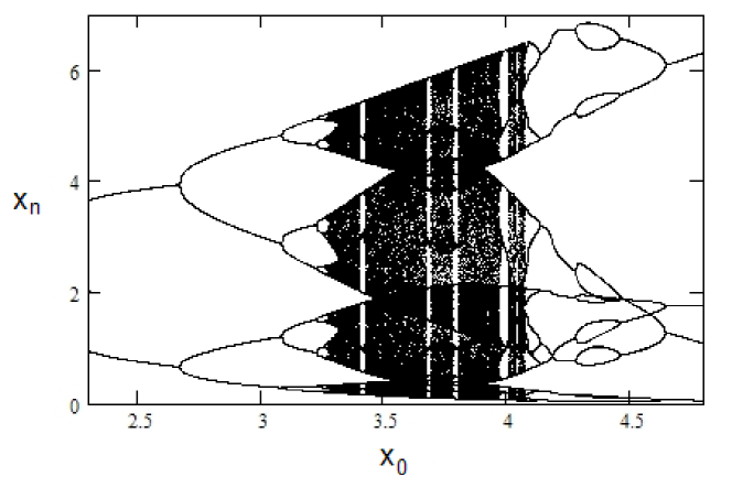
Figure 1: Bifurcations of solutions of Eq.(62) with a changing initial value; $a=4.6$ is fixed.

In Figure 1, for every grid value of $x_{0}$ in the range 2.3-4.8, the last 200 (of 300) points of the solution $\{x_{n}\}$ are plotted vertically. In this figure, stable solutions with periods 2, 4, 8, 12 and 16 can be easily identified. All of the solutions that appear in Figure 1 represent coexisting stable orbits of Eq.(62). There are also periodic and non-periodic solutions which do not appear in Figure 1 because they are unstable (e.g., the fixed point $\bar{x}=2.3$). Additional bifurcations of both periodic and non-periodic solutions occur outside the range 2.3-4.8 which are not shown in Figure 1.

Understanding the behavior for solutions of Eq.(62) is made easier when we look at its SC factorization given by (61a) and (61b). Here $k=1$ and

$$\psi_{0}(t)=e^{-t},\quad\psi_{1}(t)=te^{-t},\quad\beta_{n}=e^{a}\text{ for all }n.$$

Thus (59) takes the form

$$\psi_{0}(t)^{c}\psi_{1}(t) =t^{c^{2}}\text{ for all }t>0$$

$$e^{-ct}te^{-t} =t^{c^{2}}\text{ for all }t>0$$

The last equality is true if $c=-1,$ which leads to the form symmetry

$$h_{1}(t)=t^{-1}\psi_{0}(t)^{-1}=\frac{1}{te^{-t}}\Rightarrow H(u_{0},u_{1})=\frac{u_{0}}{u_{1}e^{-u_{1}}}$$

and SC factorization

$$r_{n+1} =\frac{e^{a}}{r_{n}},\quad r_{0}=x_{0}h_{1}(x_{-1})=\frac{x_{0}}{x_{-1}e^{-x_{-1}}}$$ (63)

$$x_{n+1} =\frac{r_{n+1}}{h_{1}(x_{n})}=r_{n+1}x_{n}e^{-x_{n}}.$$ (64)

All solutions of (63) with $r_{0}\neq e^{a/2}$ are periodic with period 2:

$$\left\{r_{0},\frac{e^{a}}{r_{0}}\right\}=\left\{\frac{x_{0}}{x_{-1}e^{-x_{-1}}},\frac{x_{-1}e^{a-x_{-1}}}{x_{0}}\right\}.$$

Hence the orbit of each nontrivial solution $\{x_{n}\}$ of (62) in the plane is restricted to the pair of curves

$$\xi_{1}(t)=\frac{e^{a}}{r_{0}}te^{-t}\quad\text{and\quad}\xi_{2}(t)=r_{0}te^{-t}.$$ (65)

Now, if $x_{-1}$ is fixed and $x_{0}$ changes, then $r_{0}$ changes proportionately to $x_{0}$. These changes in initial values are reflected as changes in parameters in (64). The orbits of the one dimensional map $bte^{-t}$ where $b=r_{0}$ or $e^{a}/r_{0}$ exhibit a variety of behaviors as the parameter $b$ changes according to well-known rules such as the fundamental ordering of cycles and the occurrence of chaotic behavior with the appearnce of period-3 orbits when $b$ is large enough; see, e.g., [3], [5], [14], [22]. Eq.(64) splits these behaviors evenly over the pair of curves (65) as the initial value $x_{0}$ changes; see Figure 2 which shows the orbits of (62) for two different initial values $x_{0}$ with $a=4.6;$ the first 100 points of each orbit are discarded in these images so as to highlight the asymptotic behavior of each orbit. The splitting over the pair of curves $\xi_{1},\xi_{2}$ also explains why odd periods do not appear in Figure 1.

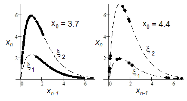
Figure 2: Two of the orbits in Figure 1 shown here on their loci of two curves $\xi_{1}$, $\xi_{2}$ in the state space.

Example 5. We now combine different types of form symmetry to show that Eq.(35) in Example 3 has the FTF property. If we assume that

$$a>0,\ x_{0}>x_{-1}>x_{-2},\ x_{0}\geq 0$$ (66)

then the multiplicative group $(0,\infty)$ of positive real numbers is the invariant set of Eq.(36). Since (36) is obviously separable over $(0,\infty)$, we check equality (59) in Corollary 2 with $\psi_{0}(t)=t$ and $\psi_{1}(t)=1/t$:

$$t^{c-1}=t^{c^{2}}\quad\text{for all }t>0.$$

This condition holds if $c^{2}-c+1=0.$ The quadratic has complex roots

$$c_{\pm}=\frac{1\pm i\sqrt{3}}{2}$$

so by Corollary 2, Eq.(36) has a form symmetry

$$H(u_{0},u_{1})=u_{0}h_{1}(u_{1}),\quad\text{where }h_{1}(t)=t^{c_{+}}t^{-1}=t^{-c_{-}}$$

and an SC factorization

$$r_{n+1} =ar_{n}^{c_{+}},\quad r_{0}=t_{0}h_{1}(t_{-1})$$ (67)

$$t_{n+1} =r_{n+1}t_{n}^{c_{-}}.$$ (68)

The three equations (67), (68) and (37) establish that Eq.(35) has the FTF property with a factorization

$$r_{n+1} =ar_{n}^{c_{+}},$$

$$t_{n+1} =ar_{n}^{c_{+}}t_{n}^{c_{-}},$$

$$x_{n+1} =ar_{n}^{c_{+}}t_{n}^{c_{-}}+x_{n}.$$

It is noteworthy that in spite of the occurrence of complex exponents, this system generates positive solutions from positive initial values. This fact may seem less surprising if Eq.(36) is transformed into a linear equation (with complex eigenvalues) by taking logarithms as in the beginning of this section.

Remark. Under the added restrictions (66), Corollary 2 may also be applied to Eq.(33) of Example 2 to obtain an SC factorization using the separable type of form symmetry. Is this SC factorization different from that in Example 2? To see that they are in fact the same, let $\psi_{0}(t)=t^{2}$ and $\psi_{1}(t)=1/t$ in the equality (59) and require that

$$t^{2c-1}=t^{c^{2}}\quad\text{for all }t>0.$$

This holds if $c$ is a root of the quadratic $c^{2}-2c+1=0,$ i.e., $c=1.$ Thus using (60) we calculate the form symmetry as

$$H(u_{0},u_{1})=u_{0}h_{1}(u_{1}),\quad\text{where }h_{1}(t)=t^{1}t^{-2}=t^{-1}.$$

This is just the HD1 form symmetry giving the same SC factorization as in Example 2.

Department of Mathematics, Virginia Commonwealth University, Richmond, Virginia 23284-2014, USA

Email: hsedagha@vcu.edu

References

- [1] Agarwal, R.P., Difference Equations and Inequalities, 2nd. ed., Dekker, New York, 2000.
- [2] Alseda, L. and Llibre, J. Periods for triangular maps, Bull. Austral. Math. Soc., 47 (1993) 41-53.
- [3] Block, L. and Coppel, W.A., Dynamics in One Dimension, Springer, New York, 1992.
- [4] Byrnes, G.B., Sahadevan, R., Quispel, G.R.W., Factorizable Lie symmetries and the linearization of difference equations, Nonlinearity, 8 (1995) 443-459.
- [5] Collet, P. and Eckmann, J.P., Iterated Maps on the Interval as Dynamical Systems, Birkhauser, Boston, 1980.
- [6] Dehghan, M., Kent, C.M., Mazrooei-Sebdani, R., Ortiz, N.L. and Sedaghat, H., Monotone and oscillatory solutions of a rational difference equation containing quadratic terms, J. Difference Eqs. and Appl., to appear.
- [7] Dehghan, M., Kent, C.M., Mazrooei-Sebdani, R., Ortiz, N.L. and Sedaghat, H., Dynamics of rational difference equations containing quadratic terms, J. Difference Eqs. and Appl., 14 (2008) 191-208.
- [8] Elaydi, S.N., An Introduction to Difference Equations (2nd ed.) Springer, New York, 1999.
- [9] Hydon, P.E., Symmetries and first integrals of ordinary difference equations, Proc. R. Soc. Lond. A 456 (2000) 2835-2855.
- [10] Kent, C.M. and Sedaghat, H., Convergence, periodicity and bifurcations for the two-parameter absolute difference equation, J. Difference Eqs. and Appl., 10 (2004) 817-841.
- [11] Kloeden, P.E., On Sharkovsky’s cycle coexistence ordering, Bull. Austral. Math. Soc., 20 (1979) 171-177.
- [12] Kocic, V.L. and Ladas, G., Global Behavior of Nonlinear Difference Equations of Higher Order with Applications, Kluwer, Dordrecht, 1993.
- [13] Levi, D., Trembley, S. and Winternitz, P., Lie point symmetries of difference equations and lattices, J. Phys. A: Math. Gen., 33 (2000) 8507-8523.
- [14] Li, T.Y., and Yorke, J.A., Period three implies chaos, Amer. Math. Monthly, 82 (1975) 985-992.
- [15] Maeda, S., The similarity method for difference equations, IMA J. Appl. Math. 38 (1987) 129-134.
- [16] Sedaghat, H., Global behaviors of rational difference equations of orders two and three with quadratic terms, J. Difference Eqs. and Appl. (2008) to appear.
- [17] Sedaghat, H., Periodic and chaotic behavior in a class of nonlinear difference equations, Proceedings of the 11th Int’l. Conf. Difference Eqs. Appl., Kyoto, Japan (2006) to appear.
- [18] Sedaghat, H., Reduction of order of separable second order difference equations with form symmetries, Int. J. Pure and Appl. Math., to appear.
- [19] Sedaghat, H., Difference equations with order-reducing form symmetries, to appear.
- [20] Sedaghat, H., All homogeneous second order difference equations of degree one have semiconjugate factorizations, J. Difference Eqs. and Appl., 13 (2007) 453-456.
- [21] Sedaghat, H., Every homogeneous difference equation of degree 1 admits a reduction in order, J. Difference Eqs. and Appl., to appear.
- [22] Sedaghat, H., Nonlinear Difference Equations: Theory with Applications to Social Science Models, Kluwer, Dordrecht, 2003.