Geometry of the energy landscape and folding transition in a simple model of a protein

Abstract

A geometric analysis of the global properties of the energy landscape of a minimalistic model of a polypeptide is presented, which is based on the relation between dynamical trajectories and geodesics of a suitable manifold, whose metric is completely determined by the potential energy. We consider different sequences, some with a definite protein-like behavior, a unique native state and a folding transition, and the others undergoing a hydrophobic collapse with no tendency to a unique native state. The global geometry of the energy landscape appears to contain relevant information on the behavior of the various sequences: in particular, the fluctuations of the curvature of the energy landscape, measured by means of numerical simulations, clearly mark the folding transition and allow to distinguish the protein-like sequences from the others.

I Introduction

Protein folding is one of the most fundamental and challenging open questions in molecular biology. Proteins are polymers made of amino acids and since the pioneering experiments by Anfinsen and coworkers Anfinsen it has been known that the sequence of amino acids—also called the primary structure of the protein—uniquely determines its native state, or tertiary structure, i.e., the compact configuration the protein assumes in physiological conditions and which makes it able to perform its biological tasks proteinbook . To understand how the information contained in the sequence is translated into the three-dimensional native structure is the core of the protein folding problem, and its solution would allow one to predict a protein’s structure from the sole knowledge of the amino acid sequence: being the sequencing of a protein much easier than experimental determination of its structure, it is easy to understand the impact such a solution would have on biochemistry and molecular biology. Moreover, solving the protein folding problem would make it possible to engineer proteins which fold to any given structure (what is commonly referred to as the inverse folding problem), which in turn would mean a giant leap in drug design. Despite many remarkable advances in the last decades, the protein folding problem is still far from a solution proteinbook .

A polymer made of amino acids is referred to as a polypeptide. However, not all polypeptides are proteins: only a very small subset of all the possible sequences of the twenty naturally occurring amino acids have been selected by evolution. According to our present knowledge, all the naturally selected proteins fold to a uniquely determined native state, but a generic polypeptide does not (it rather has a glassy-like behavior). Then the following question naturally arises: what makes a protein different from a generic polypeptide? or, more precisely, which are the properties a polypeptide must have to behave like a protein, i.e., to fold into a unique native state regardless of the initial conditions, when the environment is the correct one? This question is, obviously, much less general than the whole folding problem, nonetheless if one could give it an answer it would surely help in the quest of a solution to the folding problem.

This question has aroused a lot of interest in the recent years: the energy landscape picture has emerged as crucial in this respect. Energy landscape, or more precisely potential energy landscape, is the name commonly given to the graph of the potential energy of interaction between the microscopic degrees of freedom of the system Wales ; the latter is a high-dimensional surface, but one can also speak of a free energy landscape when only its projection on a small set of collective variables (with a suitable average over all the other degrees of freedom) is considered Wales . Before having been applied to biomolecules, this concept has proven useful in the study of other complex systems, especially of supercooled liquids and of the glass transition naturecomplex . The basic idea is very simple, yet powerful: if a system has a rugged, complex energy landscape, with many minima and valleys separated by barriers of different height, its dynamics will experience a variety of time scales, with oscillations in the valleys and jumps from one valley to another. Then one can try to link special features of the behavior of the system (i.e., the presence of a glass transition, the separation of time scales, and so on) to special properties of the landscape, like the topography of the basins around minima, the energy distribution of minima and saddles connecting them and so on. Anyway, a complex landscape yields a complex dynamics, where the system is very likely to remain trapped in different valleys when the temperature is not so high. This is consistent with a glassy behavior, but a protein does not show a glassy behavior, it rather has relatively low frustration. This means that there must be some property of the landscape such to avoid too much frustration. This property is commonly referred to as the folding funnel funnel : though locally rugged, the low-energy part of the energy landscape is supposed to have an overall funnel shape so that most initial conditions are driven towards the correct native state. The dynamics must then be such as to make this happen in a reasonably fast and reliable way, i.e., non-native minima must be efficiently connected to the native state si that trapping in the wrong onfiguration si unlikely.

However, a direct visualization of the energy landscape is impossible due to its high dimensionality, and its detailed properties must be inferred indirectly. A possible strategy is a local one: one searches for the minima of the landscape and then for the saddles connecting different minima. This is practically unfeasible for accurate all-atom potential energies, but may become accessible for minimalistic potentials. Minimalistic models are those where the polymer is described at a coarse-grained level, as a chain of $N$ beads where $N$ is the number of amino acids; no explicit water molecules are considered and the solvent is taken into account only by means of effective interactions among the monomers. Minimalistic models can be relatively simple, yet in some cases yield very accurate results which compare well with experiments Clementi_review ; Clementi . The local properties of the energy landscape of minimalistic models have been recently studied (see e.g. Refs. Miller_Wales ; BonginiRampioni ; Bongini1 ; keyes ; peyrard ; Luccioli ) and very interesting clues about the structure of the folding funnel and the differences between protein-like heteropolymers and other polymers have been found: in particular, it has been shown that a funnel-like structure is present also in homopolymers, but what makes a big difference is that in protein-like systems jumps between minima corresponding to distant configurations are much more favoured dynamically Bongini2 .

The above mentioned local strategy to analyze energy landscapes requires however a huge computational effort if one wants to obtain a good sampling. So the following question arises: is there some global property of the energy landscape which can be easily computed numerically as an average along dynamical trajectories and which is able to identify polymers having a protein-like behavior? We shall show in the following that such a quantity indeed exists, at least for the minimalistic model we considered, and that it is of a geometric nature. In particular, the fluctuations of a suitably defined curvature of the energy landscape clearly mark the folding transition while do not show any remarkable feature when the polymer undergoes a hydrophobic collapse without a preferred native state. This is at variance with thermodynamic global observables, like the specific heat, which show a very similar behavior in the case of a folding transition and of a simple hydrophobic collapse.

The paper is organized as follows: we first describe the geometric approach to energy landscapes, then we discuss the model studied and our results. A final section is devoted to some comments. A short, preliminary account of a part of the results presented here has already been given in mazzoni_casetti .

II Geometry of the energy landscape

The intuitive reason why geometric information on the landscape, and especially curvature, could be relevant to the problem of folding is that the dynamics on a landscape would be heavily affected by the local curvature: minima of the energy landscape are associated to positive curvatures and stable dynamics, while saddles involve negative curvatures, at least along some direction, thus implying some instability. One can reasonably expect that the arrangement and detailed properties of minima and saddles might reflect in some global feature of the distribution of curvatures of the landscape, when averaged along a typical trajectory.

The definition of the curvature of a manifold $M$ depends on the choice of a metric $g$ Nakahara ; DoCarmo : once the couple $(M,g)$ is given, a covariant derivative and a curvature tensor $R(e_{i},e_{j})$ can be defined; the latter measures the noncommutativity of the covariant derivatives in the coordinate directions $e_{i}$ and $e_{j}$. A scalar measure of the curvature at any given point $P\in M$ is the the sectional curvature

$$K(e_{i},e_{j})=\langle R(e_{i},e_{j})e_{j},e_{i}\rangle~{},$$ (1)

where $\langle\cdot,\cdot\rangle$ stands for the scalar product. At any point of an $N$-dimensional manifold there are $N(N-1)$ sectional curvatures, whose knowledge determines the full curvature tensor at that point. One can however define some simpler curvatures (paying the price of losing some information): the Ricci curvature $K_{R}(e_{i})$ is the sum of the $K$’s over the $N-1$ directions orthogonal to $e_{i}$,

$$K_{R}(e_{i})=\sum_{j=1}^{N}K(e_{i},e_{j})~{},$$ (2)

and summing also on the $N$ directions $e_{i}$ one gets the scalar curvature

$${\cal R}=\sum_{i=1}^{N}K_{R}(e_{i})=\sum_{i,j=1}^{N}K(e_{i},e_{j})~{};$$ (3)

then, $\frac{K_{R}}{N-1}$ and $\frac{{\cal R}}{N(N-1)}$ can be considered as average curvatures at a given point.

Although one expects the association between minima and positive curvatures on the one side and negative curvatures along some directions and saddles on the other side to be essentially true for most choices of the metric, a particular choice of $g$ among the many possible ones must be made in order to perform explicit calculations. The most immediate choice would probably be that of considering as our manifold $M$ the $N$-dimensional surface $z=V(q_{1},\ldots,q_{N})$ itself, i.e., the graph of the potential energy $V$ as a function of the $N$ coordinates $q_{1},\ldots,q_{N}$ of the configuration space, and to define $g$ as the metric induced on that surface by its immersion in $\mathbb{R}^{N+1}$. Although perfectly reasonable, this choice has two drawbacks: $(i)$ the explicit expressions for the curvatures in terms of derivatives of $V$ are rather complicated and $(ii)$ the link between the properties of the dynamics and the geometry is not very precise, i.e., one cannot prove that the geometry completely determines the dynamics and its stability. For these reasons we left the investigation of this particular geometry to future work and we considered a choice of $(M,g)$ such that the link between geometry and dynamics is more clear.

Let us now describe this metric and its relation to dynamics. We shall mention only the most important results, referring the reader to the review paper physrep for the details.

II.1 Geometry and dynamics

Let us consider a standard Hamiltonian system, with Hamiltonian function of the form

$$H=\sum_{i=1}^{N}\frac{p_{i}^{2}}{2m_{i}}+V(q_{1},...,q_{N}),$$ (4)

where $q_{i}$ and $p_{i}$ are the canonically conjugated coordinates and momenta of the system, $N$ is the number of degrees of freedom and $m_{i}$ are the masses; in the following we shall consider $m_{i}=1$ $\forall i$.

The trajectories of the system (4) in configuration space can be seen as geodesics of a Riemannian manifold: this classic result is based on the variational formulation of dynamics Arnold . Hamilton’s principle states that the natural motions of a system are the extrema of the action functional

$$S=\int L\ dt\ ,$$ (5)

where $L$ is the Lagrangian function of the system,

$$L=\frac{1}{2}\delta_{ij}\dot{q}^{i}\dot{q}^{j}-V(q_{1},...,q_{N})$$ (6)

(summation on repeated indices is understood from now on); on the other hand, the geodesics of a Riemannian manifold are extrema of the length functional

$$\ell=\int ds\ ,$$ (7)

where $s$ is the arc-length defined by

$$ds^{2}=g_{ij}\,dq^{i}\,dq^{j}~{},$$ (8)

so that we can identify the geodesics with the physical trajectories of the system by choosing a suitable metric $g$ linking action and length.

The typical example of such a metric is the Jacobi metric on the $N$-dimensional configuration space $M$,

$$g_{ij}=2\left[E-V(q_{1},...,q_{N})\right]\,\delta_{ij}~{},$$ (9)

where $E$ is the total energy of the system. Starting from Eqs. (9) one can easily show that the geodesic equations, i.e., the Euler-Lagrange equations for the length functional (7), whose expression in local coordinates is

$$\frac{d^{2}q^{i}}{ds^{2}}+\Gamma_{jk}^{i}\frac{dq^{j}}{ds}\frac{dq^{k}}{ds}=0\ ,$$ (10)

where the $\Gamma$’s are the Christoffel symbols, become Newton’s equations

$$\frac{d^{2}q^{i}}{dt^{2}}=-\frac{\partial V}{\partial q_{i}}\ .$$ (11)

However, the choice of such a metric is not unique. A particularly useful metric was introduced by Eisenhart in 1929 Eisenhart ; it is the one we used and we are going to describe in the following.

II.1.1 Eisenhart metric and landscape curvature

One could be tempted to identify actions with lengths by considering the configuration spacetime, i.e., $M\times\mathbb{R}$, with local coordinates $(q_{0},q_{1},...,q_{N})$ where $q_{0}$ is the time coordinate, however it can’t be easily done. Eisenhart’s idea was to further enlarge the configuration spacetime with another dimension, i.e., to consider $M\times\mathbb{R}^{2}$ with local coordinates $(q_{0},q_{1},...,q_{N},q_{N+1})$, and to endow this manifold with a pseudo-Riemannian metric whose arc-length is

$$ds^{2}=\delta_{i,j}dq^{i}dq^{j}-2V(q)(dq^{0})^{2}+2dq^{0}dq^{N+1}\ .$$ (12)

This is the Eisenhart metric Eisenhart : its metric tensor will be referred to as $g_{E}$ and its components are

$$g_{E}=\left(\begin{array}[]{ccccc}-2V(q)&0&\cdots&0&1\\ 0&1&\cdots&0&0\\ \vdots&\vdots&\ddots&\vdots&\vdots\\ 0&0&\cdots&1&0\\ 1&0&\cdots&0&0\\ \end{array}\right)$$ (13)

as can be derived by Eq. (12).

The connection between the geodesics of this metric and the natural motions of the system is contained in a theorem (for a detailed statement and proof see Lich ) stating that the natural motions of a Hamiltonian dynamical system are obtained by projecting on the configuration space-time $M\times\mathbb{R}$ those geodesics of $(M\times\mathbb{R}^{2},g_{E})$ whose arc-lengths are positive definite and affinely parametrized with time (remember that $q^{0}=t$), i.e., given by:

$$ds^{2}=c_{1}^{2}\,dt^{2}\ ,$$ (14)

where $c_{1}$ is an arbitrary constant. Condition (14) can be equivalently cast as a condition on $q^{N+1}$, that is

$$q^{N+1}=\frac{c_{1}^{2}}{2}t+c_{2}^{2}-\int_{0}^{t}L\,dt~{},$$ (15)

where $c_{2}$ is another arbitrary constant. Conversely, every point of $M\times\mathbb{R}^{2}$ such that its projection on the configuration spacetime lies on a a physical trajectory of the system and $q^{N+1}$ is given by (15) belongs to an affinely parametrized geodesic of $(M\times\mathbb{R}^{2},g_{E})$.

The nonzero Christoffel symbols of the Eisenhart metric are

$$\Gamma_{00}^{i}=-\Gamma_{0i}^{N+1}=\frac{\partial V}{\partial q_{i}}~{},$$ (16)

so that the geodesic equations (10) become

$$\frac{d^{2}{q^{0}}}{ds^{2}} = 0\ ,$$ (17)

$$\frac{d^{2}q^{i}}{ds^{2}}+\Gamma_{00}^{i}\frac{dq^{0}}{ds}\frac{dq^{0}}{ds} = 0\ ,$$ (18)

$$\frac{d^{2}q^{N+1}}{ds^{2}}+\Gamma_{0i}^{N+1}\frac{dq^{0}}{ds}\frac{dq^{i}}{ds} = 0\ ,$$ (19)

and using $ds=dt$, i.e., condition (14) with $c_{1}=1$, we have

$$\frac{d^{2}q^{0}}{dt^{2}} = 0\ ;$$ (20)

$$\frac{d^{2}q^{i}}{dt^{2}} = -\frac{\partial V}{\partial q_{i}}\ ;$$ (21)

$$\frac{d^{2}q^{N+1}}{dt^{2}} = -\frac{dL}{dt}\ .$$ (22)

Equation (20) states that $q^{0}=t$, the $N$ equations (21) are Newton’s equations and Eq. (22) is the differential version of Equation (15).

The nonvanishing components of the curvature tensor are

$$R_{0i0j}=\partial_{i}\partial_{j}V~{};$$ (23)

it can then be shown that the Ricci curvature (2) in the direction of motion, i.e., in the direction of the velocity vector $v$ of the geodesic, is given by

$$K_{R}(v)=\triangle V~{},$$ (24)

where $\triangle V$ is the Laplacian of the potential $V$, and that the scalar curvature ${\cal R}$ identically vanishes.

We note that $K_{R}(v)$ is nothing but a scalar measure of the average curvature “felt” by the system during its evolution; we will refer to it simply as $K_{R}$ dropping the dependence on the direction. Another feature of $K_{R}$ is its very simple analytical expression which simplifies both analytical calculation and numerical estimates. It is also worth noticing that expression (24) is a very natural and intuitive measure of the curvature of the energy landscape, as it can be seen as a naive generalization of the curvature $f^{\prime\prime}(x)$ of the graph of a one-variable function to the graph of the $N$-dimensional function $V(q_{1},...,q_{N})$: the Laplacian of the function. However, the previous discussion shows that it is much more than a naive measure of curvature and that it contains information on the local neighborhood of the dynamical trajectories. This can be exploited to gain information on the stability of the dynamics. However, we shall not go on along this line here, and we refer the reader to the review physrep as well as to the monograph marco_book .

The Ricci curvature defined in Eq. (24) will be the quantity we shall use to characterize the geometry of the energy landscape.

III Model and numerical simulations

Let us now describe the model whose energy landscape geometry we studied. We considered a simple model able to describe protein-like polymers as well as polymers with no tendency to fold; the different behaviors being selected upon the choice of the amino acidic sequence. The model we chose is a minimalistic model originally introduced by Thirumalai and coworkers Thirumalai . In order to characterize its energy landscape geometry, we sampled the value of the Ricci curvature $K_{R}$ defined in Eq. (24) along its dynamical trajectories. We shall now describe the model and the details of the numerical simulations; then we shall report on the results.

III.1 The model

The Thirumalai model is a three-dimensional off-lattice model of a polypeptide which has only three different kinds of amino acids: polar (P), hydrophobic (H) and neutral (N). The potential energy is

$$V(\vec{r}_{1},\ldots,\vec{r}_{N}) = V_{\text{bond}}(|{\vec{r}}_{i}-{\vec{r}}_{i-1}|)+V_{\text{angular}}(|{\vartheta}_{i}-{\vartheta}_{i-1}|)$$ (25)

$$+ V_{\text{dihedral}}({\psi}_{i})+V_{\text{non-bonded}}({\vec{r}}_{1},\ldots,{\vec{r}}_{N})$$

where

$$V_{\text{bond}} = \sum_{i=1}^{N-1}\frac{k_{r}}{2}(|{\vec{r}}_{i}-{\vec{r}}_{i-1}|-a)^{2}~{};$$ (26)

$$V_{\text{angular}} = \sum_{i=1}^{N-2}\frac{k_{\vartheta}}{2}(|{\vartheta}_{i}-{\vartheta}_{i-1}|-\vartheta_{0})^{2}~{};$$ (27)

$$V_{\text{dihedral}} = \sum_{i=1}^{N-3}\left\{A_{i}[1+\cos\psi_{i}]+B_{i}[1+\cos(3\psi_{i})]\right\}~{};$$ (28)

$$V_{\text{non-bonded}} = \sum_{i=1}^{N-3}\sum_{j=i+3}^{N}V_{ij}(|{\vec{r}}_{i,j}|)~{},$$ (29)

where $\vec{r}_{i}$ is the position vector of the $i$-th monomer, $\vec{r}_{i,j}=\vec{r}_{i}-\vec{r}_{j}$, $\vartheta_{i}$ is the $i$-th bond angle, i.e., the angle between $\vec{r}_{i+1}$ and $\vec{r}_{i}$, $\psi_{i}$ the $i$-th dihedral angle, that is the angle between the vectors $\hat{n}_{i}=\vec{r}_{i+1,i}\times\vec{r}_{i+1,i+2}$ and $\hat{n}_{i+1}=\vec{r}_{i+2,i+1}\times\vec{r}_{i+2,i+3}$, $k_{r}=100$, $a=1$, $k_{\vartheta}=20$, $\vartheta_{0}=105^{\circ}$, $A_{i}=0$ and $B_{i}=0.2$ if at least two among the residues $i,i+1,i+2,i+3$ are N, $A_{i}=B_{i}=1.2$ otherwise. As to $V_{ij}$, we have

$$V_{ij}=\frac{8}{3}\left[\left(\frac{a}{r}\right)^{12}+\left(\frac{a}{r}\right)^{6}\right]$$ (30)

if $i,j=\text{P},\text{P}$ or $i,j=\text{P},\text{H}$,

$$V_{ij}=4\left[\left(\frac{a}{r}\right)^{12}-\left(\frac{a}{r}\right)^{6}\right]$$ (31)

if $i,j=\text{H},\text{H}$ and

$$V_{ij}=4\left(\frac{a}{r}\right)^{6}$$ (32)

if either $i$ or $j$ are N Thirumalai .

\psfrag{ylabel}{$V_{\text{dihedral}}(\psi)$}\psfrag{xlabel}{$\psi~{}(\text{rad})$}\includegraphics[width=227.62204pt,angle={-90},clip={true}]{potential.ps}

Figure 1: (Color online) V${}_{\text{dihedral}}$ vs. dihedral angle $\psi_{i}$: the red (lower) curve corresponds to the case in which at least two out of the four beads defining the angle $\psi_{i}$ are neutral (N), the blue (upper) curve to the other cases; the central minimum corresponds to a planar configuration of the four monomers defining $\psi_{i}$.

The meaning of the different terms of the potential energy is the following. V${}_{\text{bond}}$ accounts for the covalent bonds between the $\alpha$-carbons on the main protein chain, V${}_{\text{angular}}$ for the energy cost associated to deviations from the preferred bond angle between two neighbors on the chain, and V${}_{\text{dihedral}}$ describes the contribution of non planar structures to the energy. These terms have very different energy scales, due to the different strengths of the bonds, and the dihedral term V${}_{\text{dihedral}}$ strongly depends on the local amino acidic composition: the formation of non-planar structures (turns and so on) is favored by the presence of neutral monomers (see Fig. 1). All the interactions between non-neighboring monomers along the chain, including hydrophobic effective interactions, are described by the Lennard-Jones term $V_{\text{non-bonded}}$. The presence of different energy scales as well as the competition between bonding terms (favoring planar, straight configurations) and non-bonded interactions (favoring compact configurations when the polymer is mostly hydrophobic) suggest that the energy landscape is very complicated and the possibilty of a high degree of frustration in the system: however, it is clear that these features will strongly depend on the details of the aminoacidic sequence. For example, a hydrophobic homopolymer is expected to be more frustrated than a heteropolymer, because in the homopolymer case there is a large number of compact configurations which are energetically equivalent (at least as long as the non-bonded contribution to the energy is considered) while with a heteropolymer different compact configurations have different energies.

III.2 Simulations and results

Although the identity between trajectories and projections of the geodesics of $(M,g_{E})$ only holds if the dynamics is the Newtonian one, a Langevin dynamics, obtained by adding to the deterministic force $\nabla V$ a random force according to the fluctuation-dissipation theorem and a friction term proportional to the velocity, is a more reasonable model of the dynamics of a polymer in aqueous solution when the solvent degrees of freedom are not taken into account explicitly. Since we are interested not in the details of the time series of $K_{R}$ along a particular trajectory but only in its statistical distribution, we may expect that also a sampling obtained using the Langevin dynamics gives the same information on the geometry of the landscape. To check this assumption we let the system evolve with both a Newtonian dynamics (using a symplectic algorithm MacLachlan to integrate the equations of motion) and a Langevin dynamics (using the same algorithm—a modified Verlet—and parameters as in Ref. Thirumalai ) obtaining very similar results. This is reasonable because at equilibrium, i.e., for sufficiently long simulations, the Langevin dynamics (resp. Newtonian dynamics) samples the phase space according to a canonical (resp. microcanonical) distribution, and the two distributions are expected to be equivalent for large systems, apart from small deviations due to finite size effects.

In the following we shall refer only to results obtained with Langevin dynamics.

III.2.1 Simulation details

All the numerical results will be given in natural units defined as follows: the unit of length $\ell$ is equal to the equilibrium bond length (i.e., the equilibrium distance between two consecutive beads in the chain), the unit of energy $\varepsilon$ is the hydrophobic interaction scale, i.e., the depth of the Lennard-Jones potential well between two hydrophobic beads, the unit of mass $m$ is the mass of the residues. Then the time unit becomes $\ell\sqrt{m/\varepsilon}$ and the temperature unit is $\varepsilon/k_{B}$ where $k_{B}$ is the Boltzmann constant.

As already mentioned above, the integration algorithm we used to solve numerically the Langevin equations of motion is the modified Verlet given in Ref. Thirumalai . The time step was $\Delta t=5\times 10^{-3}$. Each run was $1.7\times 10^{7}$ time steps long, including equilibration. Results for a given temperature were obtained averaging over 8 different randomly chosen initial conditions. The mean and rms fluctuation of the observables, and in particular of the curvature of the landscape $K_{R}$, was estimated from the histogram of the sampled values. Statistical errors on the single run have been estimated dividing each run in 12 tranches, considered as independent, and then propagated to the final result.

III.2.2 Sequences

We considered six different sequences of “amino acids” H, P and N: four of 22 monomers, $S^{22}_{\text{g}}$, $S^{22}_{\text{b}}$, $S^{22}_{\text{i}}$, $S^{22}_{\text{h}}$, and two sequences of 46 monomers, $S^{46}_{\text{h}}$, $S^{46}_{\text{g}}$. The six sequences are listed in Table 1. Sequences $S^{22}_{\text{g}}$ and $S^{46}_{\text{g}}$ had already been identified as good folders Thirumalai ; Thirumalai2 and our simulations confirmed this finding: below a given temperature $S^{22}_{\text{g}}$ (resp. $S^{46}_{\text{g}}$) always reached the same $\beta$-sheet-like structure (resp. $\beta$-barrel-like structure). A plot of the number of native contacts $N_{n}$ (see Sec. III.2.3 for the definition) as a function of the temperature for these two proteinlike sequences is reported in Fig. 2. Homopolymers $S^{22}_{\text{h}}$ and $S^{46}_{\text{h}}$, on the other hand, showed a hydrophobic collapse but no tendency to reach a particular configuration in the collapsed phase, as expected. Sequence $S^{22}_{\text{b}}$ (which has the same overall composition of $S^{22}_{\text{g}}$ rearranged in a different sequence) behaved as a bad folder and did not reach a unique native state, while $S^{22}_{\text{i}}$ was constructed by us to show a somehow intermediate behavior between good and bad folders: it always forms the same structure involving the middle of the sequence, while the beginning and the end of the chain fluctuate also at low temperature.

name		sequence
S${}^{22}_{\text{g}}$		PH9(NP)2NHPH3PH
S${}^{22}_{\text{b}}$		PHNPH3NHNH4(PH2)2PH
S${}^{22}_{\text{i}}$		P4H5NHN2H6P3
S${}^{22}_{\text{h}}$		H22
S${}^{46}_{\text{g}}$		P(HP)5N3H9N3(HP)4N3H9
S${}^{46}_{\text{h}}$		H46

Table 1: The six sequences considered. (X)_y means that X is repeated $y$ times.

III.2.3 Estimate of collapse and folding temperatures

The hydrophobic collapse temperature $T_{\theta}$ and the folding temperature $T_{f}$ (the latter only for the two protein-like sequences S${}_{\text{g}}^{22}$ and S${}_{\text{g}}^{46}$ and for the “intermediate” sequence S${}_{\text{i}}^{22}$) were estimated in a standard way as follows.

$T_{\theta}$ has been estimated as the temperature where the specifc heat shows a peak. The rationale for this definition is that the hydrophobic collapse of a polymer becomes a thermodynamic phase transition, commonly referred to as $\theta$ transition, in the thermodynamic limit of an infinite number of monomers degennes ; at the critical temperature (usually denoted by $T_{\theta}$, notation that we adopt also for our finite size case) the specific heat diverges, and the specific heat peak we observed in our systems is nothing but the precursor of this divergence. One could define a collapse temperature also by monitoring quantities directly related to the collapse itself, as the gyration radius or the end-to-end distance of the polymer; we checked that the estimates of $T_{\theta}$ obtained this way were perfectly compatible with those based on the specific heat.

At variance with the collapse transition, the folding transition does not have any corresponding “true” phase transition in the thermodynamic limit, simply because no thermodynamic limit exists for a protein: we cannot increase the number of amino acids of a protein beyond any limit whithout destroying its protein-like behavior Dill ; CecconiBurioni . From the point of view of statistical physics, protein folding may be considered a genuine finite-size phenomenon. Any estimate of the folding temperature $T_{f}$ will then be somehow fuzzy. We adopted one of the various possible protocols. First, we defined the fraction $N_{n}$ of native contacts in any configuration as

$$N_{n}=\frac{1}{n_{c}}\sum_{i=1}^{N}\sum_{j=i+2}^{N}\Theta(d_{s}-r_{ij})\Theta(d_{s}-r^{n}_{ij})~{},$$ (33)

where $r_{ij}$ is the distance between the $i$-th and $j$-th residues, $r_{ij}^{n}$ the distance between the same residues in the reference (native) configuration, $n_{c}=\sum_{i=1}^{N}\sum_{j=i+2}^{N}\Theta(d_{s}-r^{n}_{ij})$ the total number of contacts in the native configuration, and $d_{s}$ the threshold distance below which two beads are considered in contact: the value of $d_{s}$ is the mean distance between beads in contact in the native configuration. Then, $T_{f}$ is defined as the temperature of the inflection point in the curve $N_{n}(T)$. These curves are shown in Fig. 2.

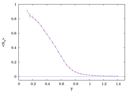
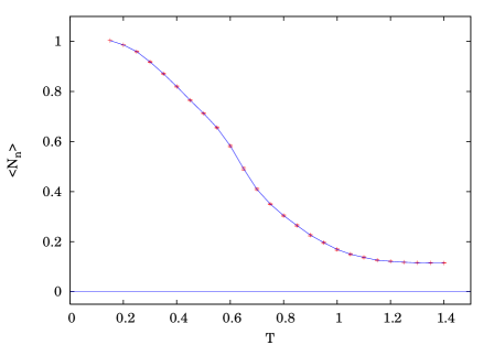
Figure 2: (Color online) $\langle N_{n}\rangle$ vs. temperature $T$ for the two good folders: $S^{22}_{\text{g}}$ (left), $S^{46}_{\text{g}}$ (right). The curves are a guide to the eye.

The estimated $T_{f}$ and $T_{\theta}$ for the six sequences are given in Table 2. Errors on $T_{\theta}$ (resp. $T_{f}$) have been obtained by estimating the interval of the position of the peak in $c_{V}(T)$ (resp. in the derivative of $N_{n}(T)$) compatible with the errors on the numerical data for $c_{V}$ (resp. $N_{n}$).

sequence	$T_{\theta}$	$T_{f}$
S${}^{22}_{\text{g}}$	$0.65\pm 0.05$	$0.55\pm 0.1$
S${}^{22}_{\text{b}}$	$0.55\pm 0.15$	none
S${}^{22}_{\text{i}}$	$0.75\pm 0.1$	$0.7\pm 0.2$
S${}^{22}_{\text{h}}$	$0.65\pm 0.05$	none
S${}^{46}_{\text{g}}$	$0.65\pm 0.025$	$0.65\pm 0.05$
S${}^{46}_{\text{h}}$	$0.70\pm 0.025$	none

Table 2: The collapse ($T_{\theta}$) and folding ($T_{f}$) temperatures for the six sequences considered.

We note that, for the two sequences where folding occurs, $T_{f}\approx T_{\theta}$ (indeed $T_{f}=T_{\theta}$ within the estimated errors). This is not surprising at all since in general $T_{f}\leq T_{\theta}$, and one expects the folding to be more efficient if $T_{f}/T_{\theta}\approx 1$ because in this situation the polymer approaches the native state immediately when the temperature is lowered below $T_{\theta}$, reducing the possibility of misfolding in non-native compact configurations keyes .

III.2.4 Thermodynamic and geometric observables

As to standard thermodynamic observables, all the sequences showed very similar behaviors: to give an example, in Fig. 3 we compare the specific heat $c_{V}$ of the homopolymer $S^{22}_{\text{h}}$ and of the good folder $S^{22}_{\text{g}}$: both exhibit a peak at the transition, and on the sole basis of this picture it would be hard to discriminate between a simple hydrophobic collapse and a folding. The same happens in the case of the longer homopolymer $S^{46}_{\text{h}}$ and the good folder $S^{46}_{\text{g}}$ (Fig. 4).

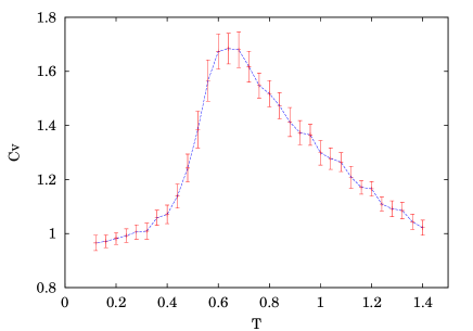
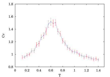
Figure 3: (Color online) Specific heat $c_{V}$ vs. temperature $T$ for the homopolymer $S^{22}_{\text{h}}$ (left) and for the good folder $S^{22}_{\text{g}}$ (right). The curves are a guide to the eye.

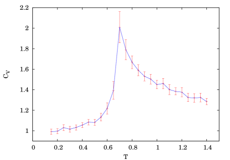
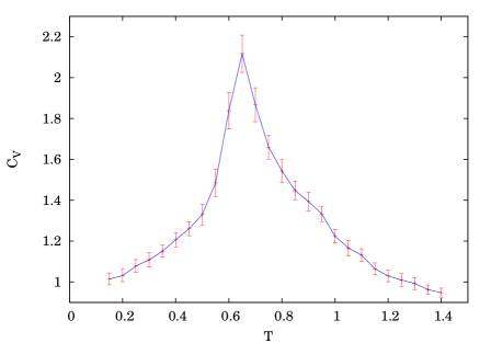
Figure 4: (Color online) As in Fig. 3 for the homopolymer $S^{46}_{\text{h}}$ (left) and the good folder $S^{46}_{\text{g}}$ (right).

On the other hand, a dramatic difference between the homopolymers and the good folders shows up if we consider the geometric properties of the landscape. In particular, a lot of information appears to be encoded in the fluctuations of the Ricci curvature $K_{R}$, i.e., of the Laplacian of the potential energy—see Eq. (24). We defined a relative adimensional curvature fluctuation $\sigma$ as

$$\sigma=\frac{\sqrt{\frac{1}{N}\left(\langle K_{R}^{2}\rangle_{t}-\langle K_{R}\rangle_{t}^{2}\right)}}{\frac{1}{N}\langle K_{R}\rangle_{t}}$$ (34)

where $\langle\cdot\rangle_{t}$ stands for a time average: in Fig. 5 we plot $\sigma$ as a function of the temperature $T$ for the homopolymer $S^{22}_{\text{h}}$ and for the good folder $S^{22}_{\text{g}}$. A clear peak shows up in the case of the good folder, close to the folding temperature $T_{f}$ below which the system is mostly in the native state, while no particular mark of the hydrophobic collapse can be seen in the case of the homopolymer. A similar situation happens for the longer sequences, the good folder $S^{46}_{\text{g}}$ and the homopolymer $S^{46}_{\text{h}}$ (Fig. 6).

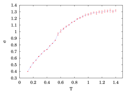
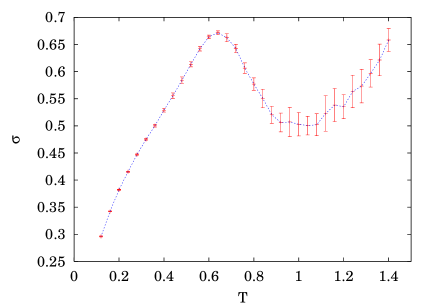
Figure 5: (Color online) Relative curvature fluctuation $\sigma$ vs. temperature $T$ for the homopolymer $S^{22}_{\text{h}}$ (left) and for the good folder $S^{22}_{\text{g}}$ (right). The curves are a guide to the eye.

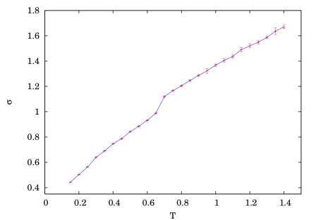
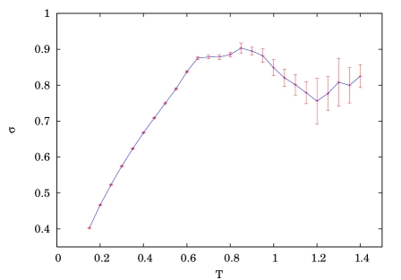
Figure 6: (Color online) As in Fig. 5 for the homopolymer $S^{46}_{\text{h}}$ and the proteinlike sequence $S^{46}_{\text{g}}$.

The relative curvature fluctuation $\sigma$ of the energy landscape appears then to be a good marker of the presence of a folding transition, at least in the simple model considered here. We stress that the comparison between sequences of length 22 and 46 clearly indicates that the peak in $\sigma$ is really related to the folding and not to the hydrophobic collapse, because $\sigma$ for the long homopolymer $S^{46}_{\text{h}}$ is even smoother than in the case of the short homopolymer $S^{22}_{\text{h}}$, at variance with the specific heat which develops a sharper peak, consistently with the fact that the system is closer to the situation where a thermodynamic $\theta$-transition exists.

In the case of the longer sequence (Fig. 6) the peak in the curvature fluctuations appears more structured: it seems to be the superposition of two peaks, one at $T_{f}\approx T_{\theta}$ and another, even higher, at $T\simeq 0.85$ where the specific heat shows a “shoulder”. This may be related to the fact that the good folder $S^{46}_{\text{g}}$ seems to reach its native state—a $\beta$-barrel made of two $\beta$-sheets—in two steps: first, at $T\simeq 0.85$, the two $\beta$-sheets form but still are free to move the one respect to the other, then, at $T_{f}$, the two sheets fold into the native $\beta$-barrel. This interpretation of the folding process as composed of two steps is corroborated by the results on the gyration radius as a function of $T$ (data not shown). The curvature fluctuations seem then to indicate both steps of folding with two separate peaks which superimpose on each other to give the structure observed in Fig.  6.

As to the other sequences, for the bad folder $S^{22}_{\text{b}}$, $\sigma(T)$ is not as smooth as for the homopolymers, but only a very weak signal is found at $T\simeq 0.4$, lower than $T_{\theta}$; below this temperature the systems seems to behave as a glass. For the “intermediate” sequence $S^{22}_{\text{i}}$ a peak is present at the “quasi-folding” temperature, although considerably broader than in the case of $S^{22}_{\text{g}}$ (see Fig. 7).

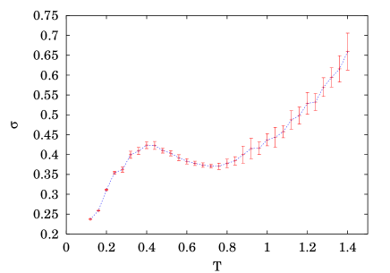
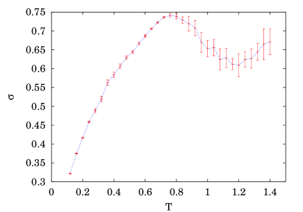
Figure 7: (Color online) $\sigma(T)$ for the sequence $S^{22}_{\text{b}}$ (on the left) and for the sequence $S^{22}_{\text{i}}$ (on the right). The curves are a guide to the eye.

III.3 A closer look at the curvature of the landscape

Where does the peak in $\sigma(T)$ near $T_{f}$ come from? To find clues towards an answer we may have a closer look at the properties of the curvature of the energy landscape. Looking at the time series of the curvature $K_{R}(t)$ for the two sequences $S^{22}_{\text{g}}$ and $S^{22}_{\text{h}}$, i.e., the good folder and the homopolymer of length 22, respectively, a clear difference shows up when we consider data sampled close to the transition temperatures, $T_{f}$ and $T_{\theta}$, respectively (Fig. 8).

Figure 8: $K_{R}(t)$ for the homopolymer $S^{22}_{\text{h}}$ at $T\approx T_{\theta}$ (on the left) and for the protein-like sequence $S^{22}_{\text{g}}$ at $T\approx T_{f}$ (on the right).

In the homopolymer, $K_{R}(t)$ oscillates in an apparently random fashion around a constant mean value; the data reported in Fig. 8 (left panel) have been taken at $T\approx T_{\theta}$, but—in the case of the homopolymer—they are not qualitatively different from those taken at any other temperature. On the contrary, the curvature signal of the protein-like sequence near $T_{f}$ (right panel in Fig. 8) is much more structured: there are several time windows where the curvature oscillates around a mean value which is considerably lower than the global one, and in these windows also the amplitude of the fluctuations is smaller.

Figure 9: $K_{R}(t)$ for the protein-like sequence $S^{22}_{\text{g}}$ at $T\simeq 0.68$, i.e., at the temperature of the peak in the relative curvature fluctuations $\sigma(T)$.

This effect is even more visible at the temperaure of the peak in the curvature fluctuations $\sigma(T)$ (which is slightly larger than the estimated $T_{f}$, although within the estimated errorbar), as shown in Fig. 9, and leads to an asymmetric distribution of the values of $K_{R}$, resulting in “anomalously large” fluctuations which are at the origin of the peak of $\sigma(T)$ close to $T_{f}$. Histograms of the distributions of $K_{R}$ for the homopolymer at $T\approx T_{\theta}$ and for the sequence $S^{22}_{\text{g}}$ at the temperature of the peak in the fluctuations, $T\simeq 0.68$, are shown in Fig. 10. Also the distribution of curvatures for the homopolymer is asymmetric, but the asymmetry is considerably lower than in the good folder case.

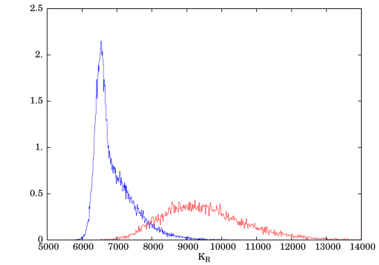
Figure 10: (Color online) Normalized distributions of $K_{R}$ for the homopolymer $S^{22}_{\text{h}}$ at $T\approx T_{\theta}$ (broad histogram) and for the protein-like sequence $S^{22}_{\text{g}}$ at $T\simeq 0.68$ (peaked histogram). The values in the vertical axis must be multiplied by $10^{-7}$. The skewness of the distributions is 0.6 for the homopolymer case and 1.4 for the protein-like case.

We interpret these data as direct indications of the presence of two macroregions in the energy landscape, one corresponding to the native state and the other—charatcterized by a smaller average curvature—corresponding to the unfolded state. Then the dynamics is effectively two-state: close to $T_{f}$, the system often jumps between the two basins and this explains the behavior of the observed time series of $K_{R}$. This interpretation is supported also by the following observations. First, the average curvature is a decreasing function of $T$ (Fig. 11); second, comparing the instantaneous values of the curvature and of the number of native contacts (defined in Eq. 33) we clearly see that the time windows where the curvature is lower correspond to zero native contacts, thus indicating that the system is in the unfolded state (Fig. 12).

This suggests that an effective description of this system in terms of a coarse-grained energy landscape should be possible: work is in progress along this direction model_1d .

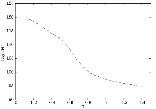
Figure 11: (Color online) Average curvature (per degree of freedom) $\langle K_{R}\rangle/N$ for the protein-like sequence $S^{22}_{\text{g}}$ as a function of $T$.

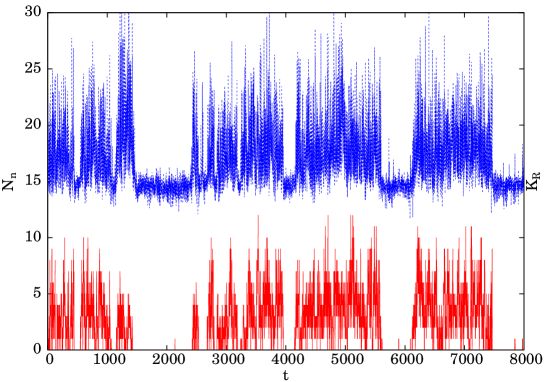
Figure 12: (Color online) Synopsis of the instantaneous values of the curvature $K_{R}$ (upper curve) and of the number of native contacts $N_{n}$ (lower curve) for the protein-like sequence $S^{22}_{\text{g}}$ in a simulation run at $T\simeq 0.68$.

IV Concluding remarks

Studying six different sequences of a minimalistic model of a protein, we have shown that a geometric quantity which measures the amplitude of the curvature fluctuations of the energy landscape, $\sigma$, when plotted as a function of the temperature $T$ shows a dramatically different behavior when the system undergoes a folding transition with respect to when only a hydrophobic collapse is present; $\sigma(T)$ can thus be used to mark the folding transition and to identify good folders, within the model considered here.

It must be stressed that no knowledge of the native state is necessary to define $\sigma$, and that it can be computed with the same computational effort needed to obtain the specific heat and other thermodynamic observables. This means that using e.g. reweighting histogram techniques one can reliably estimate the behavior of $\sigma$ as a function of $T$ using few simulation runs at properly chosen temperatures, if not a single one. Hence, if tested successfully on other, maybe more refined models of proteins, the calculation of the curvature fluctuations might prove a useful tool in the search of protein-like sequences. Preliminary results on more refined minimalistic models noi_cecilia completely confirm the scenario presented here.

In case numerical evidence accumulates and/or general theoretical arguments become available in favor of our suggestion that the peak in the curvature fluctuations is a generic marker of a protein-like behavior, then this method could provide, for example, a fast and reasonably cheap numerical tool to make a preliminary discrimination between sequences that are likely to be protein-like and the others. This may be useful not only when trying to understand the general features of energy landscapes of minimalistic models, but also for tasks of more applicative interest like assessing the relevance of point mutations in a sequence.

We have shown indications that the presence of a peak in the curvature fluctuations when the system undergoes a folding is a consequence of the effective two-state dynamics of this system close to the folding transition. On the basis of the sole results presented here such an interpretation can not be considered as definitive; nonetheless, it is confirmed by preliminary results on an effective model of the system studied here, which will be discussed in a forthcoming paper model_1d . It must also be noticed that higher curvature fluctuations imply in general a higher degree of instability of the dynamics (see physrep ), as expected near $T_{f}$ where the system has essentially the same probabilty of being in two very different states, folded or unfolded. A deeper investigation of the instability properties of the dynamics close to the folding transition would probably yield more interesting information.

Apart from the possible applications of $\sigma(T)$ as a diagnostic tool, and even more as giving indications about the global structure of the energy landscape, the results we have presented here may also be interesting because open a connection between the folding transition and symmetry-breaking phase transition. The behavior of $\sigma(T)$ observed here for the good folders is remarkably close to that exhibited by finite systems undergoing a symmetry-breaking phase transition in the thermodynamic limit TdF_geometry , while the case of the homopolymers is similar to that of a Berežinskij-Kosterlitz-Thouless transition. This suggests that the folding of a proteinlike heteropolymer does share some features of “true” symmetry-breaking phase transitions—at least those features that show up already in finite systems—although no singularity in the thermodynamic limit occurs, because proteins are intrinsically finite objects Dill ; CecconiBurioni . The behavior of $\sigma(T)$ in systems with thermodynamic phase transitions has been interpreted in terms of topological changes of the manifolds where the dynamics of the system “lives” cccp ; franz (see also physrep ; marco_book and kastner_rmp for a review). Work is in progress to understand whether such a topological interpretation can be extended also to the case of the folding transition, although it has no infinite-system, thermodynamic limit counterpart.

- (1) C. Anfinsen, Science 181, 223 (1973).
- (2) A. Finkelstein and O. B. Ptitsyn, Protein physics (Academic Press, London, 2002).
- (3) D. J. Wales, Energy landscapes (Cambridge University Press, Cambridge, 2004).
- (4) P. G. Debenedetti and F. H. Stillinger, Nature 410, 259 (2001).
- (5) J. N. Onuchic, P. G. Wolynes, Z. Luthey-Schulten, and N. D. Socci, Proc. Natl. Acad. Sci. USA 92, 3626 (1995).
- (6) W. H. Press, S. A. Teukolsky, W. T. Vetterling, and B. P. Flannery, Numerical recipes (Cambridge University Press, Cambridge, 1992).
- (7) T. S. Grigera, A. Cavagna, I. Giardina, and G. Parisi, Phys. Rev. Lett. 88, 055502 (2002).
- (8) C. Clementi, Curr. Op. Struct. Biol. 17, 1 (2007).
- (9) P. Das, S. Matysiak, and C. Clementi, Proc. Natl. Acad. Sci. USA 102, 10141 (2005).
- (10) M. A. Miller and D. J. Wales, J. Chem. Phys. 111, 6610 (1999).
- (11) L. Bongini, R. Livi, A. Politi, and A. Torcini, Phys. Rev. E 68, 061111 (2003).
- (12) L. Bongini and A. Rampioni, Gene 347, 231 (2005).
- (13) J. Gil Kim and T. Keyes, J. Phys. Chem. B 111, 2647 (2007).
- (14) M. Nakagawa and M. Peyrard, Proc. Natl. Acad. Sci. USA 103, 5279 (2006); Phys. Rev. E 74, 041916 (2006).
- (15) A. Imparato, S. Luccioli, and A. Torcini, Phys. Rev. Lett. 99, 168101 (2007).
- (16) L. Bongini, R. Livi, A. Politi, and A. Torcini, Phys. Rev. E 72, 051929 (2005).
- (17) L. N. Mazzoni and L. Casetti, Phys. Rev. Lett. 97, 218104 (2006).
- (18) M. Nakahara, Geometry, Topology and Physics (IOP Publishing, London, 2003).
- (19) M. P. do Carmo, Riemannian geometry (Birkhauser, Boston, 1992).
- (20) V. I. Arnol’d, Mathematical methods of classical mechanics (Springer, New York, 1989).
- (21) L. P. Eisenhart, Ann. Math. 30, 591 (1929).
- (22) A. Lichnerowicz, Théories rèlativistes de la gravitation et de l’éléctromagnétisme (Masson, Paris, 1955).
- (23) L. Casetti, M. Pettini, and E. G. D. Cohen, Phys. Rep. 337, 237 (2000).
- (24) M. Pettini, Geometry and topology in Hamiltonian dynamics and statistical mechanics, Interdisciplinary applied mathematics series (Springer-Verlag, New York, 2007).
- (25) T. Veitshans, D. Klimov, and D. Thirumalai, Fold. Des. 2, 1 (1997).
- (26) P. G. de Gennes, Scaling concepts in polymer physics (Cornell University Press, London, 1979).
- (27) K. A. Dill, Biochemistry 29, 31 (1990).
- (28) R. Burioni, D. Cassi, F. Cecconi, and A. Vulpiani, Proteins 55, 529 (2004).
- (29) P. MacLachlan and P. Atela, Nonlinearity 5, 541 (1992).
- (30) J. D. Honeycutt and D. Thirumalai, Proc. Natl. Acad. Sci. USA 87, 3527 (1990).
- (31) L. N. Mazzoni, R. Franzosi, L. Casetti, and C. Clementi, in preparation.
- (32) L. N. Mazzoni and L. Casetti, in preparation.
- (33) L. Caiani, L. Casetti, C. Clementi, G. Pettini, M. Pettini, and R. Gatto, Phys. Rev. E 57, 3886 (1998).
- (34) L. Caiani, L. Casetti, C. Clementi, and M. Pettini, Phys. Rev. Lett. 79, 4361 (1997).
- (35) R. Franzosi, L. Casetti, L. Spinelli, and M. Pettini, Phys. Rev. E 60, R5009 (1999).
- (36) M. Kastner, Rev. Mod. Phys. 80, 167 (2008).