Analysis of coupled heat and moisture transfer in masonry structures

Abstract

Evaluation of effective or macroscopic coefficients of thermal conductivity under coupled heat and moisture transfer is presented. The paper first gives a detailed summary on the solution of a simple steady state heat conduction problem with an emphasis on various types of boundary conditions applied to the representative volume element – a periodic unit cell. Since the results essentially suggest no superiority of any type of boundary conditions, the paper proceeds with the coupled nonlinear heat and moisture problem subjecting the selected representative volume element to the prescribed macroscopically uniform heat flux. This allows for a direct use of the academic or commercially available codes. Here, the presented results are derived with the help of the SIFEL  (SIimple Finite Elements) system.

, , ,

1 Introduction

An extensive experimental and numerical analysis of Charles Bridge in Prague has been performed only recently to identify the most severe external actions on the bridge, see e.g. [17, 21, 24]. Among others the loading due to spatially and temporarily varying temperature and moisture changes appeared to be of paramount importance as these effects proved as crucial factors responsible for the nucleation and further development of cracks in the bridge. Owing to the complexity of historical masonry structures the problem is often addressed in a strictly uncoupled format. Distribution of the temperature field in the macroscopic structure needed for the actual non-linear thermo-mechanical analysis can be obtained from an independent solution of the macroscopic steady-state heat conduction problem [17]. This step, however, requires the knowledge of the macroscopic coefficients of thermal conductivity, and possibly their influence on actual temperature and moisture content - the principal objective of the research presented.

When dealing with these problems, the application of homogenization techniques is inevitable [18]. Solving a set of problem equations on a meso-scale (a composition of stone blocks and mortar) provides us with up-scaled macroscopic equations. They include a number of effective (macroscopic) transport parameters, which are necessary for a detailed analysis of the state of a structure as a whole. A reliable methodology of the prediction of these quantities is one of the main goals of our contribution. Any (multi-scale) approach to coupled heat and moisture transfer draws on a cogent description of transport phenomena. An extensive review of this topic can be found in [23]. Averaging theories (a micromechanics-based approach), primarily formulated in [8, 9], can be regarded as a counterpart to phenomenological ones (a macromechanics-based approach), see [5, 2]. Both approaches are explained in detail in [16]. Contrary to these trends, phenomenological models are still preferred to averaging ones, namely calculating the heat and moisture transfer in building materials.

As outlined in [23], the models for the description of water and water vapor transfer can broadly be classified into three main categories, namely convection models, diffusion models and hybrid models. The recognized convection model is that of Philip and de Vries, see e.g. [19]. A variety of diffusion models were developed based on Krischer’s original version [12]. A certain drawback of this category lies in the absence of cross-effects between the heat and moisture transport. Krischer’s model was improved by many authors. Let us at least introduce Künzel and Kiessl’s model [14]. Because of the lack of space it is impossible to comment on further approaches such as hybrid models or complex models that require the application of irreversible thermo-mechanics, [23].

While models for transport processes have been developed during several decades, the computational methods for multi-scale modeling of these processes in masonry on meso and macro scales have emerged only recently. Moreover, most of them are prevailingly confined to the effective macroscopic description for heat conduction and employ the perturbation method to describe the fluctuations of temperature throughout the heterogeneous material. Different situations are analyzed using the homogenization method, which lead to different macroscopic descriptions in [1]. Boutin’s model analyzing the microstructural influence on heat conduction belongs to the same category [4]. It is shown that the higher order terms introduce successive gradients of temperature and tensor characteristics of the microstructure, which result in non-local effects. An original approach to homogenization of transient heat transfer for some composite materials is proposed in [10]. In that paper, the stochastic second moment perturbation method is used in conjunction with the finite element method. Probably the most complex multi-scale analysis for pure heat transfer in heterogeneous solids is offered in [18]. The authors established a macro to micro transition in terms of the applied boundary conditions and likewise a micro to macro transition formulated in the form of consistent averaging relations. See also [22] for a similar study with applications to textile composites.

Homogenization strategies for coupled heat and mass transfer are rather an exception, see e.g. [10], and more or less belong to the modeling of a micro to meso rather than a meso to macro transition and vice versa. Therein, the condition for a non-homogenizable situation, i.e. when it is impossible to find a macroscopic equivalent description, is also addressed.

While setting up the numerical solution of the homogenization problem is relatively straightforward, its execution may prove rather complicated if only standard (academic or commercial) finite element codes are available. Therefore, apart from the determination of the influence of temperature and moisture content on effective thermal conductivities, the present contribution will also be concerned with a strategy of predicting the desired effective properties when employing such numerical tools that are unable to directly meet the specifics of the homogenization problem formulated in the framework of the first-order homogenization approach. To combine the two goals of this paper, the following topics will be discussed:

• In Section 2 we open the subject by reviewing the basic formulas related to first-order homogenization clearly identifying the essential similarities between the mechanical and heat conduction problem. Therein and also in Section 3 the steady state conditions are assumed in the derivation of individual equations. Certain restrictions on the local temperature field to comply with the assumed macroscopic heat flux or temperature gradient being uniform over a certain representative volume element (RVE) are summarized.

• Numerical treatment of the theoretical formulation is then presented in Section 3 to provide estimates of the effective thermal conductivities by solving a simple steady state heat conduction problem. The main objective of this section is to address the effect of boundary conditions on the resulting homogenized properties. The fact that these properties are essentially invariant with respect to the choice of particular boundary conditions opens the way to the solution of the coupled heat and moisture problem using the SIFEL finite element code, a typical representative of the finite element software not specifically developed for the solution of the homogenization problem. Implementation of the loading and boundary conditions into such codes is therefore also discussed.

• The essentials of theoretical formulation as well as some numerical results are presented in Section 4 clearly illustrating the effect of moisture on thermal conductivity and their dependence on varying material parameters, such as relative humidity and initial temperature. Here, unlike the previous sections, the analysis is carried out under transient conditions. The presented results suggest that the predicted effective thermal conductivities are almost insensitive to the changes in the macroscopic temperature gradient. This is rather appealing, particularly in view of the expected use of the homogenized properties in the solution of an independent macroscopic steady state heat conduction problem to provide space variation of the temperature field within the macroscopic structure (e.g. Charles Bridge in Prague), which in turn is used in the actual mechanical analysis [17].

• Finally, the essential findings are summarized in Section 5.

In Section 2, the standard indicial notation is used such that $t_{,i}$ represents a derivative of a scalar quantity $t$ with respect to a coordinate $x_{i}$. The summation over the repeated indexes is assumed. As more typical of the discretized form of the governing equations using the finite element method, we adopt in Section 3 the matrix-vector notation such that the symbol $\{\mathsf{a}\}$ is reserved for a vector and $\left[\mathsf{A}\right]$ is employed for a matrix representation, respectively  [3]. The symbol $\{\mathsf{\nabla{\it t}}\}=\displaystyle{\left\{\frac{\partial{t}}{\partial{x}},\frac{\partial{t}}{\partial{y}},\frac{\partial{t}}{\partial{z}}\right\}^{\sf T}}$ then represents the gradient of $t$ and $\{\mathsf{\cdot}\}^{\sf T},\left[\mathsf{\cdot}\right]^{\sf T}$ stands for the transpose vector or matrix, respectively. Finally, the symbol $\dot{t}$ used in Section 4 represents the time derivative of a given quantity $t$.

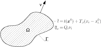
Figure 1: A representative volume element with macroscopic loading conditions

2 Fundamentals of homogenization

Consider a representative volume element $|\Omega|$ in Fig. 1 loaded over the boundary $\Gamma$ either by the prescribed temperature $\overline{t}$ derived from a uniform macroscopic temperature gradient $T_{,i}$ or by a normal heat flux $\overline{q}_{\nu}$ consistent with the macroscopic uniform heat flux $Q_{i}$ such that

$$\overline{t} = t(\mbox{\boldmath$x$}^{0})+T_{,i}(x_{i}-x_{i}^{0})\hskip 28.45274pt\mbox{ on }\Gamma,$$

$$\overline{q}_{\nu} = Q_{i}\nu_{i}\hskip 105.84428pt\mbox{ on }\Gamma,$$ (1)

where $\nu_{i}$ represents the $i$-th component of the outward unit normal. 

In such a case, the local temperature field admits the following decomposition

$$t(\mbox{\boldmath$x$})=t(\mbox{\boldmath$x$}^{0})+T_{,i}(x_{i}-x_{i}^{0})+t^{*}(\mbox{\boldmath$x$}),$$ (2)

where $T_{,i}$ are components of the macroscopically uniform temperature gradient vector and $t^{*}(\mbox{\boldmath$x$})$ is the fluctuation of the local temperature field. Finally, the temperature $t(\mbox{\boldmath$x$}^{0})$ at the reference point $\mbox{\boldmath$x$}^{0}$ is introduced to specify the distribution of the local temperature field uniquely. This term plays an important role when a fully coupled multi-scale analysis is considered and/or when the instantaneous effective thermal conductivities depend on the current temperature. If, however, we seek only for temperature independent homogenized properties, like in Section 3, this term becomes irrelevant and can be safely omitted.

Eq. (2) immediately follows from the relation between the temperature gradients of individual fields

$$t_{,i}(\mbox{\boldmath$x$})=T_{,i}+t^{*}_{,i}(\mbox{\boldmath$x$}).$$ (3)

The micro-temperature gradient averaged over the volume $|\Omega|$ of the representative volume element

$$\langle t_{,i}\rangle=\frac{1}{|\Omega|}\int_{\Omega}t_{,i}(\mbox{\boldmath$x$})\,{\mathrm{d}}\Omega(\mbox{\boldmath$x$})=T_{,i}+\frac{1}{|\Omega|}\int_{\Omega}t^{*}_{,i}(\mbox{\boldmath$x$})\,{\mathrm{d}}\Omega(\mbox{\boldmath$x$}),$$ (4)

yields a scale transition relation, see e.g. [18],

$$\langle t^{*}_{,i}\rangle=\frac{1}{|\Omega|}\int_{\Omega}t^{*}_{,i}(\mbox{\boldmath$x$})\,{\mathrm{d}}\Omega(\mbox{\boldmath$x$})=\frac{1}{|\Omega|}\int_{\Gamma}t^{*}(\mbox{\boldmath$x$})\nu_{i}(\mbox{\boldmath$x$})\,{\mathrm{d}}\Gamma(\mbox{\boldmath$x$})=0.$$ (5)

The boundary integral disappears providing either the fluctuation part of the temperature field equals zero (in the case of fully prescribed temperature and/or normal heat flux boundary conditions) or the periodic boundary conditions, i.e. the same values of $t^{*}$ on opposite sides of a rectangular RVE, are enforced on $\Gamma$.

When discussing the micro to macro scale transition it is worth mentioning an analogy between the basic quantities related to the heat conduction problems (i.e. the negative values of temperature gradients $(-t_{,i})$ or $(-T_{,i})$ and fluxes $q_{i}$ or $Q_{i}$ as their conjugate measures) and the corresponding quantities applied to mechanical problems (strains $\varepsilon_{ij}$ or $E_{ij}$ and the conjugate stress measures $\sigma_{ij}$ or $\Sigma_{ij}$). While homogenization of mechanical problems benefits from the Hill lemma

$$\langle{\varepsilon}_{ij}\sigma_{ij}\rangle={E}_{ij}\Sigma_{ij},$$ (6)

where $E_{ij},\Sigma_{ij}$ are macroscopically uniform strain and stress tensors and $\varepsilon_{ij},\sigma_{ij}$ are their local counterparts, the Fourier inequality [15] is used to obtain an equivalent representation of Eq. (6) given by

$$\langle(-t_{,i})q_{i}\rangle=-T_{,i}Q_{i},$$ (7)

which is applicable in the case of homogenization of the heat conduction problems.

Following the transformation of the volume integral in Eq. (5) to its boundary equivalent it is useful to convert the left-hand side of Eq. (7) in a similar way

$$\langle t_{,i}q_{i}\rangle = \frac{1}{|\Omega|}\int_{\Omega}t_{,i}(\mbox{\boldmath$x$})q_{i}(\mbox{\boldmath$x$})\,{\mathrm{d}}\Omega(\mbox{\boldmath$x$})=\frac{1}{|\Omega|}\int_{\Gamma}t(\mbox{\boldmath$x$})q_{i}(\mbox{\boldmath$x$})\nu_{i}(\mbox{\boldmath$x$})\,{\mathrm{d}}\Gamma(\mbox{\boldmath$x$})=$$ (8)

$$= \frac{1}{|\Omega|}\int_{\Gamma}t(\mbox{\boldmath$x$})q_{\nu}(\mbox{\boldmath$x$})\,{\mathrm{d}}\Gamma(\mbox{\boldmath$x$}).$$

The term

$$-\frac{1}{\Omega}\int_{\Omega}t(\mbox{\boldmath$x$})q_{i,i}(\mbox{\boldmath$x$})\,{\mathrm{d}}\Omega(\mbox{\boldmath$x$}),$$ (9)

has been omitted in Eq. (8) because of the balance of heat (i.e. $q_{i,i}=0$ under steady state conditions and the absence of internal heat sources).

The same boundary conditions, which satisfy Eq. (5), lead to the equivalence of the volume averaged microscopic heat flux $q_{i}$ and the macroscopic heat flux $Q_{i}$. To prove this, the well-known identity

$$\int_{\Omega}q_{i}(\mbox{\boldmath$x$})\,{\mathrm{d}}\Omega(\mbox{\boldmath$x$})=\int_{\Gamma}x_{i}q_{\nu}(\mbox{\boldmath$x$})\,{\mathrm{d}}\Gamma(\mbox{\boldmath$x$}),$$ (10)

is utilized. The following three situations can be distinguished:

• In the case of fully prescribed temperature boundary conditions, the subsequent combination of Eqs. (2), (8) and (10), in conjunction with the balance condition

  $$\int_{\Gamma}q_{\nu}(\mbox{\boldmath$x$})\,{\mathrm{d}}\Gamma(\mbox{\boldmath$x$})=0,$$ (11)

  yields

  $$\langle t_{,i}q_{i}\rangle = \frac{t(\mbox{\boldmath$x$}^{0})}{|\Omega|}\int_{\Gamma}q_{\nu}(\mbox{\boldmath$x$})\,{\mathrm{d}}\Gamma(\mbox{\boldmath$x$})+\frac{T_{,i}}{|\Omega|}\int_{\Gamma}(x_{i}-x^{0}_{i})q_{\nu}(\mbox{\boldmath$x$})\,{\mathrm{d}}\Gamma(\mbox{\boldmath$x$})=$$ (12)

  $$= \frac{T_{,i}}{|\Omega|}\int_{\Omega}q_{i}(\mbox{\boldmath$x$})\,{\mathrm{d}}\Omega(\mbox{\boldmath$x$})=T_{,i}Q_{i}.$$

  This identity implies

  $$Q_{i}=\frac{1}{|\Omega|}\int_{\Omega}q_{i}(\mbox{\boldmath$x$})\,{\mathrm{d}}\Omega(\mbox{\boldmath$x$}).$$ (13)

• A similar situation is met if normal heat flux boundary conditions are prescribed. Substituting the prescribed macroscopic flux $Q_{i}$ into Eq. (12) for $q_{i}$ immediately proves the validity of Eq. (13).

• The periodic temperature boundary conditions are typical of rectangular PUCs. From the transition relation (5), the fluctuation temperature $t^{*}$ must be the same on the opposite boundaries of PUC. As the anti-periodic normal heat flux applies to the periodic boundary conditions, Eq. (12) yields, after certain modifications, the expected result (13).

3 Macroscopic conductivity and resistivity matrices

Before proceeding with the analysis of a complex coupled nonlinear heat and moisture conduction problem we review the basic steps for the evaluation of macroscopic conductivity and resistivity matrices through the solution of a simple steady state heat conduction problem using the finite element method. This allows us to examine the influence of various boundary conditions, discussed in the previous section, on the predicted homogenized properties and further exploit these results in the next section when solving the coupled problem.

As intimated in the previous section, compare Eqs. (6) - (7), the macroscopic conductivity and resistivity matrices may be derived by analogy to the homogenized stiffness and compliance matrices which apply to mechanical analyses. Therefore, we first discuss the numerical treatment of Eq. (6), which allows the RVE being directly loaded by prescribed macroscopic uniform strain or stress fields $E_{ij}$ or $\Sigma_{ij}$, respectively. The analogous loading conditions (macroscopic temperature gradient $T_{,i}$ or macroscopic heat flux $Q_{i}$) that apply to heat conduction problem are examined next. Such loading conditions are, however, difficult to introduce directly into most finite element codes including the SIFEL program. Instead, the loading conditions of the type (1) are needed. This, on the other hand, calls for a special treatment of the boundary conditions associated with a fluctuation part of the local temperature field $t^{*}$. To elucidate this subject, a brief comment is given in the last part of this section.

3.1 Searching the solution in terms of the fluctuation part of the local temperature

To begin, consider a rectangular RVE (particular definition of an RVE will be given later in Section 3.2) subjected either to macroscopic uniform strain $\{\mathsf{E}\}$ or stress $\{\mathsf{\Sigma}\}$. Henceforth, as already mentioned in the introductory part, the standard vector-matrix notation is adopted. Limiting our attention to linear elastic theory, thus allowing for small displacements, rotations and strains only, provides the virtual work representation of Eq. (6) in the form

$$\langle\{\mathsf{\delta\varepsilon}\}{\sf{}^{T}}\{\mathsf{\sigma}\}\rangle=\{\mathsf{\delta{E}}\}{\sf{}^{T}}\{\mathsf{\Sigma}\}.$$ (14)

where the discretized form of the local strain, in analogy with Eq. (3), and stress fields are provided by

$$\{\mathsf{\varepsilon}\}=\{\mathsf{E}\}+\left[\mathsf{B_{u}}\right]\{\mathsf{r^{*}_{u}}\},\quad\{\mathsf{\sigma}\}=\left[\mathsf{L}\right]\{\mathsf{\varepsilon}\}.$$ (15)

In Eq. (15) $\{\mathsf{r_{u}^{*}}\}$ is the vector of the nodal values of the fluctuation displacement field being periodic (the same values of $\{\mathsf{r_{u}^{*}}\}$ on opposite sides of an RVE), $\left[\mathsf{B_{u}}\right]$ stores derivatives of the displacement shape functions and $\left[\mathsf{L}\right]$ is the microscopic material stiffness matrix. This equation readily suggests that the solution of Eq. (14) is searched in terms of fluctuation rather than actual displacements. Next, introducing Eq. (15) into Eq. (14) gives

$$\left<\left(\{\mathsf{\delta{E}}\}{\sf{}^{T}}+\{\mathsf{\delta{r_{u}^{*}}}\}{\sf{}^{T}}\left[\mathsf{B_{u}}\right]{\sf{}^{T}}\right)\left[\mathsf{L}\right]\left(\{\mathsf{E}\}+\left[\mathsf{B_{u}}\right]\{\mathsf{r_{u}^{*}}\}\right)\right>=\{\mathsf{\delta{E}}\}{\sf{}^{T}}\{\mathsf{\Sigma}\},$$ (16)

to be satisfied for all kinematically admissible strains $\{\mathsf{\delta{E}}\}$ and displacements $\{\mathsf{\delta{r_{u}^{*}}}\}$.

Let $\{\mathsf{E}\}$ be now the prescribed macroscopic strain vector. The above equation then reduces to (note that $\{\mathsf{\delta{E}}\}=\{\mathsf{0}\}$)

$$\langle\left[\mathsf{B_{u}}\right]{\sf{}^{T}}\left[\mathsf{L}\right]\left[\mathsf{B_{u}}\right]\rangle\{\mathsf{r_{u}^{*}}\}=-\langle\{\mathsf{B_{u}}\}{\sf{}^{T}}\left[\mathsf{L}\right]\rangle\{\mathsf{E}\},$$ (17)

to be solved for unknown nodal values of the fluctuation part of the displacement field $\{\mathsf{r_{u}^{*}}\}$. The macroscopic constitutive law can be then expressed as

$$\{\mathsf{\Sigma}\}=\langle\{\mathsf{\sigma}\}\rangle=\langle\left[\mathsf{L}\right](\{\mathsf{E}\}+\{\mathsf{B_{u}}\}\{\mathsf{r_{u}^{*}}\})\rangle=\left[\mathsf{L}\right]^{hom}\{\mathsf{E}\},$$ (18)

where $\left[\mathsf{L}\right]^{hom}$ is the homogenized (macroscopic) material stiffness matrix. Assuming e.g. plane-stress conditions the coefficients of the $3\times{3}$ matrix $\left[\mathsf{L}\right]^{hom}$ are defined as volume averages of the local fields derived from the solution of three successive elasticity problems. To that end, the representative volume element is loaded, in turn, by each of the three components of $\{\mathsf{E}\}$, while the other two vanish. The volume stress averages, Eq. (18), normalized with respect to $\{\mathsf{E}\}$ then furnish individual columns of $\left[\mathsf{L}\right]^{hom}$. Note that introduction of the periodic boundary conditions is, in this particular case, relatively simple as it is only required to assign, in the FEM terminology, the same code numbers to corresponding degrees of freedom of $\{\mathsf{r_{u}^{*}}\}$ on opposite sides of the RVE. To avoid the rigid body motion and also as a result of the application of periodic boundary conditions the rectangular RVE is fixed at all corners.

If, on the other hand, the macroscopic stress $\{\mathsf{\Sigma}\}$ is prescribed (note that in this case $\{\mathsf{\delta{E}}\}\neq\{\mathsf{0}\}$) a similar procedure is employed to arrive at a set of the following equations for unknown ${\{\mathsf{E}\}}$ and ${\{\mathsf{r}\}_{u}^{*}}$

$$\langle\left[\mathsf{L}\right]\rangle\{\mathsf{E}\}+\langle\left[\mathsf{L}\right]\left[\mathsf{B_{u}}\right]\rangle\{\mathsf{r_{u}^{*}}\} = \{\mathsf{\Sigma}\},$$

$$\langle\left[\mathsf{L}\right]\left[\mathsf{B_{u}}\right]\rangle{\sf{}^{T}}\{\mathsf{E}\}+\langle\left[\mathsf{B_{u}}\right]{\sf{}^{T}}\left[\mathsf{L}\right]\left[\mathsf{B_{u}}\right]\rangle\{\mathsf{r_{u}^{*}}\} = \{\mathsf{0}\}.$$ (19)

Here, solving for $\{\mathsf{E}\}$ from the three independent elasticity problems and again normalizing by $\{\mathsf{\Sigma}\}$ readily provides the macroscopic material compliance matrix $\left[\mathsf{M}\right]^{hom}=(\left[\mathsf{L}\right]^{hom})^{-1}$ as

$$\{\mathsf{E}\}=\left[\mathsf{M}\right]^{hom}\{\mathsf{\Sigma}\}.$$ (20)

Derivation of the effective thermal conductivities and resistivities will be now presented on the same footing taking advantage of the analogy between mechanical and heat conduction problem. To do so, we first write Eq. (7) in the form similar to Eq. (14)

$$\langle\{\mathsf{\delta\nabla{\it t}}\}{\sf{}^{T}}\{\mathsf{\it q}\}\rangle=\{\mathsf{\delta\nabla{\it T}}\}{\sf{}^{T}}\{\mathsf{\it Q}\}.$$ (21)

The discretized form of the local temperature gradient and heat flux now reads

$$\{\mathsf{\nabla{\it t}}\}=\{\mathsf{\nabla{\it T}}\}+\left[\mathsf{B_{t}}\right]\{\mathsf{r_{t}^{*}}\},\quad\{\mathsf{\it q}\}=-\left[\mathsf{\chi}\right]\{\mathsf{\nabla{\it t}}\},$$ (22)

where $\{\mathsf{r_{t}^{*}}\}$ is now the vector of nodal values of the fluctuation temperature field, $\left[\mathsf{\chi}\right]$ is the microscopic conductivity matrix and entries of the matrix $\left[\mathsf{B_{t}}\right]$ represent the derivatives of the temperature shape functions.

For the prescribed macroscopic temperature gradient $\{\mathsf{\nabla{\it T}}\}$ the equality (21) results in (compare with Eq. (17))

$$\langle\left[\mathsf{B_{t}}\right]{\sf{}^{T}}\left[\mathsf{\chi}\right]\left[\mathsf{B_{t}}\right]\rangle\{\mathsf{r_{t}^{*}}\}=-\langle\left[\mathsf{B_{t}}\right]{\sf{}^{T}}\left[\mathsf{\chi}\right]\rangle\{\mathsf{\nabla{\it T}}\},$$ (23)

and, successively, in the macroscopic relation for the heat flux

$$\{\mathsf{\it Q}\}=\langle\{\mathsf{\it q}\}\rangle=-\langle\left[\mathsf{\chi}\right](\{\mathsf{\nabla{\it T}}\}+\left[\mathsf{B_{t}}\right]\{\mathsf{r_{t}^{*}}\})\rangle=-\left[\mathsf{\chi}\right]^{hom}\{\mathsf{\nabla{\it T}}\},$$ (24)

where the homogenized conductivity matrix $\left[\mathsf{\chi}\right]^{hom}$ now follows, with the expected restrictions to two-dimensional problem, from the solution of two successive heat conduction problems in exactly the same way as already outlined for the homogenized stiffness matrix $\left[\mathsf{L}\right]^{hom}$. The periodic boundary conditions now require the same fluctuation temperatures to be ensured on opposite sides of the RVE, see also Fig. 4 and Eq. (29). In analogy to the mechanical problem a zero value of $t^{*}$ is prescribed at all corners of the RVE.

The prescribed macroscopic heat flux $\{\mathsf{\it Q}\}$ then provides, in analogy with Eq. (19),

$$-\langle\left[\mathsf{\chi}\right]\rangle\{\mathsf{\nabla{\it T}}\}-\langle\left[\mathsf{\chi}\right]\left[\mathsf{B_{t}}\right]\rangle\{\mathsf{r_{t}^{*}}\} = \{\mathsf{\it Q}\},$$

$$\langle\left[\mathsf{\chi}\right]\left[\mathsf{B_{t}}\right]\rangle{\sf{}^{T}}\{\mathsf{\nabla{\it T}}\}+\langle\left[\mathsf{B_{t}}\right]{\sf{}^{T}}\left[\mathsf{\chi}\right]\left[\mathsf{B_{t}}\right]\rangle\{\mathsf{r_{t}^{*}}\} = \{\mathsf{0}\},$$ (25)

$$\{\mathsf{\nabla{\it T}}\} = -\left[\mathsf{\Psi}\right]^{hom}\{\mathsf{\it Q}\},$$ (26)

where $\left[\mathsf{\Psi}\right]^{hom}=(\left[\mathsf{\chi}\right]^{hom})^{-1}$ is the effective (macroscopic) resistivity matrix.

3.2 Influence of boundary conditions on effective conductivities

To capture the influence of the selected type of boundary conditions consider an RVE displayed in Fig. 2. Such a meso-structure does not represent a typical masonry bonding, as in this scheme both the stone blocks and bed and head joints are regularly and uniformly distributed. It is also worth noting that such an arrangement is not perfectly periodic due to the disturbance of periodicity along the boundary. This large RVE has been deliberately chosen to demonstrate certain edge effects, which may be taken into account when homogenization is carried out using commercial and/or academic computer codes. If the RVE was perfectly periodic (i.e. one half of the boundary mortar joint was added as sketched by the dashed line in Fig. 2), then, due to the infinite periodicity, any stone block along with the adjacent part of joints shaded in Fig. 2 would be sufficient for calculating the effective value of thermal conductivity.

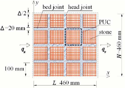
Figure 2: Meso-structure consisting of stone blocks and mortar joints

mortar	sandstone
0.87	1.9

Table 1: Phase conductivities ${\chi}[\mathrm{Wm^{-1}K^{-1}}]$ at $t=25^{0}C,\varphi=0\%$

In this simple case the coupling effects between the heat and moisture were omitted. The phase thermal conductivities are listed in Table 1. First, the effect of imperfect periodicity was studied by loading the large RVE in Fig. 2 consisting of 16 stone blocks and surrounding bed and head joints by a uniform macroscopic temperature gradient $\nabla_{x}T=1$ while setting $\nabla_{y}T=0$. Fully prescribed boundary temperatures were considered so that $t^{*}=0$. The fluctuation temperature field displayed in Fig. 3(a) was found from the solution of Eq. (23). Note that the imperfect periodicity of the RVE (the edge effect) manifests itself in slightly affecting the periodicity of the fluctuation field $t^{*}$. Fig. 3(b) shows similar results derived by assuming the RVE in terms of the PUC. Finally, the results plotted in Fig. 3(c) were generated again through the solution of the unit cell problem but incorporating the periodic boundary conditions. To avoid possible confusion the large RVE, now modified to comply with perfect periodicity, was finally examined. Both the influence of fully prescribed boundary temperatures ($t^{*}=0$ on $\Gamma$) and the periodic boundary conditions were again studied.

Large RVE	Large RVE	Large RVE	PUC	PUC
non-periodic	periodic	periodic
$t^{*}=0$ on $\Gamma$	$t^{*}=0$ on $\Gamma$	$t^{*}$-periodic	$t^{*}=0$ on $\Gamma$	$t^{*}$-periodic
1.563	1.48	1.47	1.48	1.47
Voight	1.58	$\chi_{x}^{hom}=c^{m}\chi_{x}^{m}+c^{s}\chi_{x}^{s}$
Reuss	1.39	$1/\chi_{x}^{hom}=c^{m}/\chi_{x}^{m}+c^{s}/\chi_{x}^{s}$

Table 2: Effective conductivities ${\chi}^{hom}_{x}[\mathrm{Wm^{-1}K^{-1}}]$

The corresponding effective thermal conductivities were obtained directly from the solution of Eq. (23) together with Eq. (24). Individual values are stored in Table 2 clearly suggesting, at least in this particular example, the invariance of the predicted effective thermal conductivities on the choice of specific boundary conditions. This appealing result is further exploited in Section 4.2. The Voight bound derived from a simple rule of mixture and the Reuss bound provided by an inverse rule of mixture are presented for illustration. The volume fractions of mortar $c^{m}=0.31$ and stones $c^{s}=0.69$ correspond to periodic structure (PUC in Fig. 2).

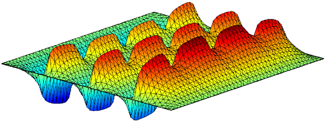
(a)

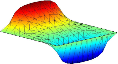
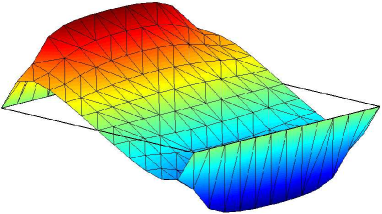
(b)	(c)

Figure 3: Fluctuation temperature field: (a) large RVE and $t^{*}=0$ (b) PUC and $t^{*}=0$ (c) PUC and $t^{*}$-periodic

3.3 Searching the solution in terms of the local temperature - periodic boundary conditions in commercial codes

Recall that the effective thermal conductivities have been obtained assuming the solution to be derived in terms of the fluctuation part $t^{*}$ of the local temperature $t$ when loading an RVE directly by the prescribed macroscopic temperature gradient $\{\mathsf{\nabla{\it T}}\}$ or by the macroscopic uniform heat flux $\{\mathsf{\it Q}\}$. The designer, however, must often rely on the use of standard finite element codes, either academic or commercial, where the loading is represented in terms of the prescribed boundary temperatures or fluxes of the type (1) and the solution is searched directly in terms of the local temperatures $t(\mbox{\boldmath$x$}),\mbox{\boldmath$x$}\in\Omega$.

Consider now the most simple case illustrated in Fig. 2, when the RVE is loaded by the uniform heat flux $|q_{\nu}|=q_{x}=Q_{x}$ along the two vertical boundaries at $x=0,x=L$ while no flow boundary conditions are specified $|q_{\nu}|=q_{y}=Q_{y}=0$ along the two horizontal boundaries at $y=0,y=H$. Eq. (13) is then immediately satisfied and the horizontal component of the effective heat conductivity is, in view of Eqs. (26) and (3), provided by

$$\chi_{x}^{hom}=-\frac{q_{x}}{\langle{t}_{,x}\rangle}.$$ (27)

If no action is taken this result corresponds to the assumption of $t^{*}=0$ on $\Gamma$. If, on the other hand, the periodic boundary conditions are on demand it is necessary proceed as follows. Consider again a two-dimensional rectangular RVE with dimensions $H$ and $L$ (see Fig. 4).

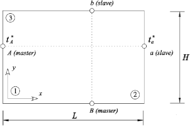
Figure 4: Conditions of periodicity

Observe that for a pair of points (e.g. $A$ - master and $a$ - slave) located on the opposite sides of the PUC the following relations hold:

$$t_{A}=\left(\frac{\partial T}{\partial y}\right)y_{A}+t^{*}_{A}+t(\mbox{\boldmath$x$}^{0}),\quad t_{a}=\left(\frac{\partial T}{\partial x}\right)L+\left(\frac{\partial T}{\partial y}\right)y_{a}+t^{*}_{a}+t(\mbox{\boldmath$x$}^{0}).$$ (28)

Taking into account the fact that the fluctuation field $t^{*}$ satisfies the periodicity condition

$$t^{*}_{a}=t^{*}_{A},$$ (29)

and subtracting corresponding terms on the opposite edges, we finally obtain (compare with [18])

$$\left(\frac{\partial T}{\partial x}\right)L = t_{a}-t_{A}=t_{2}-t_{1},$$

$$\left(\frac{\partial T}{\partial y}\right)H = t_{b}-t_{B}=t_{3}-t_{1}.$$ (30)

These conditions can be introduced into most commercial software products using the multi-point constraint equations.

Note that neither the assumption of $t^{*}=0$ on $\Gamma$ nor the periodic conditions (29) (or constraints (30)) are sufficient to specify the local temperature field uniquely. This condition is established by introducing a reference temperature $t(\mbox{\boldmath$x$}^{0})$ at an arbitrary point $\mbox{\boldmath$x$}^{0}\in\Gamma$ as indicated in Eqs. (28), recall also the opening Section 2 together with Eqs. (1)₁ and (2).

In a linear case, when the effective thermal conductivities are independent of the actual temperature, this value is arbitrary and can be set equal to zero in the selected node of the finite element mesh. In the temperature dependent problem the instantaneous effective properties might, however, be strongly influenced by the current temperature. This term then plays an important role. In an example presented in Section 4.2 a reference temperature equal to the selected initial temperature was assigned to one of the corner nodes of the finite element mesh of the large RVE in Fig. 2.

4 Effect of moisture on thermal conductivity

So far we restrained our attention to heat conduction problems under steady state conditions. To that end, the balance equation, $q_{i,i}=0$, Fourier’s law and the equivalence of heat powers on micro- and macro-scales, Eq. (7), were sufficient to derive both effective conductivity and resistivity matrices. When analyzing large structural systems, such as historical stone bridges, cathedrals and similar historical structures, the effect of moisture must be taken into consideration and, therefore, the solution of the coupled heat and moisture transfer is desirable.

4.1 Computer codes used for coupled mass and energy transfer

There exist a number of codes that allow for the description of non-linear and non-stationary material behavior as well as cross - effects when studying the moisture and heat transfer in heterogeneous infrastructures. Here we recall at least two of them. The SIFEL (SImple Finite Elements) computer code developed at our department [13] is a typical representative of programs based on finite element techniques. This program was used to derive the results presented in Section 4.2. The DELPHIN program [6, 7] is on the other hand developed on the bases of finite control volume method (FCVM). Although not specifically used in this contribution this program has proved useful in a number of verification tests.

In this section we mention two particular models implemented in the SIFEL program. The model of Lewis and Schrefler is likely the most advanced hygro-thermo-mechanical model so far employed for practical calculations of transport processes in soils and other deformed porous media. As its detailed description can be found e.g. in [16], we just summarize the basic features of this model. The complete set of model equations comprises the linear balance (equilibrium) equation formulated for a multiphase body, the energy balance equation and the equations of mass conservation for liquid water and gas. Assuming the rigidity of the solid phase, the number of fundamental unknowns in the theory of the coupled moisture and heat transfer reduces to three, namely the temperature $t$ and the pressures in the liquid and gaseous phases $p^{w}$, $p^{g}$, respectively. These unknown functions can be solved from three basic equations

• one energy balance equation,

• two equations of mass conservation.

The second model implemented in the SIFEL code is that of Künzel and Kiessl [14]. It is much simpler then the previous one and, despite the fact that the cross-effects are missing in this model, it describes all substantial phenomena and its results comply well with experimentally obtained data. For these reasons it has been chosen to carry out the case study on masonry microstructure and will be commented on in more detail in this paragraph.

Vapor diffusion and liquid transport due to differences in capillary suction stress are the main mechanisms of moisture transport. Although an interaction of liquid and vapor fluxes under very humid conditions cannot be excluded, they are treated as independent processes in this model (vapor diffusion is most important in large pores, whereas liquid transport takes place on pore surfaces, in crevices and small capillaries).

Thermo-diffusion is neglected in this model and vapor flux, $\{\mathsf{{\it q}_{v}}\}$, is described by the following equations

$$\{\mathsf{{\it q}_{v}}\}=-\delta_{p}\{\mathsf{\nabla{\it p}}\},$$ (31)

where $\delta_{p}$ is the vapor permeability of the porous material and $p$ is the vapor pressure. The liquid transport incorporates the liquid flow in the absorbed layer (surface diffusion) and in the water filled capillaries (capillary transport). The driving potential in both cases is capillary pressure (suction stress) and/or, according to Kelvin’s law, relative humidity $\varphi$. Hence, the flux of liquid water, $\{\mathsf{{\it q}_{w}}\}$, can be written as

$$\{\mathsf{{\it q}_{w}}\}=-D_{\varphi}\{\mathsf{\nabla{\varphi}}\},$$ (32)

where $D_{\varphi}=D_{w}\displaystyle{\frac{\,{\mathrm{d}}w}{\,{\mathrm{d}}\varphi}}$ is the liquid conductivity , $D_{w}=D_{w}(w/w_{f})$ is the liquid diffusivity , $\,{\mathrm{d}}w/\,{\mathrm{d}}\varphi$ is the derivative of the water retention function and $w/w_{f}$ is the water content related to the capillary saturation. Finally, the heat flux, $\{\mathsf{{\it q}_{t}}\}$, attains the following form

$$\{\mathsf{{\it q}_{t}}\}=-\chi\{\mathsf{\nabla{\it t}}\}-h_{v}\delta_{p}\{\mathsf{\nabla(\varphi{\it p}_{sat})}\},$$ (33)

where $h_{v}$ is the specific heat of evaporation and $p_{sat}$ is the saturation vapor pressure.

In this model, the resulting set of differential equations for the description of heat and moisture transfer, expressed in terms of temperature and relative humidity $\varphi$, assumed the following form:

• The energy balance equation

  $$\left(\rho c+\frac{\,{\mathrm{d}}H_{w}}{\,{\mathrm{d}}t}\right)\dot{t}=\{\mathsf{\nabla}\}{\sf{}^{T}}\left[\chi\{\mathsf{\nabla{\it t}}\}+h_{v}\delta_{p}\{\mathsf{\nabla(\varphi{\it p}_{sat})}\}\right]$$ (34)

• The conservation of mass equation

  $$\frac{\,{\mathrm{d}}w}{\,{\mathrm{d}}\varphi}\dot{\varphi}=\{\mathsf{\nabla}\}{\sf{}^{T}}\left[D_{\varphi}\{\mathsf{\nabla\varphi}\}+\delta_{p}\{\mathsf{\nabla(\varphi{\it p}_{sat})}\}\right].$$ (35)

In Eqs. (34) - (35) $\rho$ is the material density, $c$ is the specific heat capacity and $H_{w}$ is the enthalpy of material moisture. Details concerning the specification of material parameters can be found in [14]. The storage terms appear on the left hand side of Eqs. (34) and (35). The conductivity heat flux and the enthalpy flux by vapor diffusion with phase changes in Eq. (34) are strongly influenced by the moisture fields. The vapor flux in Eq. (35) is governed by both the temperature and moisture fields due to exponential changes of the saturation vapor pressure, $p_{sat}$, with temperature. Vapor and liquid convection caused by total pressure differences or gravity forces as well as the changes of enthalpy by liquid flow are neglected in this model.

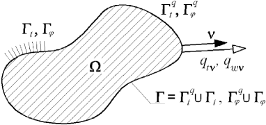
Figure 5: A two dimensional region (e.g. an RVE in Fig. 2 with prescribed heat flux)

In the SIFEL program these equations are converted to a weak formulation. Using the weighted residual statement the energy balance equation becomes

$$\int_{\Omega}w_{t}\left<\left(c+\frac{\,{\mathrm{d}}H_{w}}{\,{\mathrm{d}}t}\right)\dot{t}-\{\mathsf{\nabla}\}{\sf{}^{T}}\left[\chi\{\mathsf{\nabla{\it t}}\}+h_{v}\delta_{p}\{\mathsf{\nabla(\varphi{\it p}_{sat})}\}\right]\right>\,{\mathrm{d}}\Omega+$$

$$+\int_{\Gamma_{t}^{q}}w_{t}\left<\{\mathsf{\nu}\}{\sf{}^{T}}\left[\chi\{\mathsf{\nabla{\it t}}\}+h_{v}\delta_{p}\{\mathsf{\nabla(\varphi{\it p}_{sat})}\}\right]+\overline{q}_{t\nu}\right>\,{\mathrm{d}}\Gamma=0,$$ (36)

where $w_{t}$ is the weighting function such that $w_{t}=0$ on $\Gamma_{t}$, see Fig. 5. Applying Green’s theorem then yields

$$\int_{\Omega}\left\{w_{t}\left(c+\frac{\,{\mathrm{d}}H_{w}}{\,{\mathrm{d}}t}\right)\dot{t}+\{\mathsf{\nabla{\it w}_{t}}\}{\sf{}^{T}}\left[\chi\{\mathsf{\nabla{\it t}}\}+h_{v}\delta_{p}\{\mathsf{\nabla(\varphi{\it p}_{sat})}\}\right]\right\}\,{\mathrm{d}}\Omega+$$

$$+\int_{\Gamma_{t}^{q}}w_{t}\overline{q}_{t\nu}\,{\mathrm{d}}\Gamma=0,$$ (37)

where $\overline{q}_{t\nu}$ is the prescribed heat flux perpendicular to the boundary $\Gamma_{t}^{q}$. On $\Gamma_{t}$ the temperature $t$ is equal to its prescribed value $\overline{t}$. Vector $\{\mathsf{\nu}\}$ stores the components of the unit outward normal defined already in Section 2, see also Fig. 5.

The weak formulation for the conservation of mass can be derived analogously

$$\int_{\Omega}w_{\varphi}\left<\frac{\,{\mathrm{d}}w}{\,{\mathrm{d}}\varphi}\dot{\varphi}-\{\mathsf{\nabla}\}{\sf{}^{T}}\left[D_{\varphi}\{\mathsf{\nabla\varphi}\}+\delta_{p}\{\mathsf{\nabla(\varphi{\it p}_{sat})}\}\right]\right>\,{\mathrm{d}}\Omega+$$

$$+\int_{\Gamma_{\varphi}^{q}}w_{\varphi}\left<\{\mathsf{\nu}\}{\sf{}^{T}}\left[D_{\varphi}\{\mathsf{\nabla\varphi}\}+\delta_{p}\{\mathsf{\nabla(\varphi{\it p}_{sat})}\}\right]+\overline{q}_{w\nu}\right)\,{\mathrm{d}}\Gamma,$$ (38)

where $w_{\varphi}$ is the corresponding weighting function such that $w_{\varphi}=0$ on $\Gamma_{\varphi}$. Application of Green’s theorem finally gives

$$\int_{\Omega}\left\{w_{\varphi}\frac{\,{\mathrm{d}}w}{\,{\mathrm{d}}\varphi}\dot{\varphi}+\{\mathsf{\nabla{\it w}_{\varphi}}\}{\sf{}^{T}}\left[D_{\varphi}\{\mathsf{\nabla\varphi}\}+\delta_{p}\{\mathsf{\nabla(\varphi{\it p}_{sat})}\}\right]\right\}\,{\mathrm{d}}\Omega+$$

$$+\int_{\Gamma_{\varphi}^{q}}w_{\varphi}\overline{q}_{w\nu}\,{\mathrm{d}}\Gamma,$$ (39)

where $\overline{q}_{w\nu}$ is the prescribed flux of water perpendicular to the boundary $\Gamma_{\varphi}^{q}$. On $\Gamma_{\varphi}$ the relative humidity is again equal to its prescribed value $\overline{\varphi}$.

A detailed specification of boundary conditions used in our particular case will be given in the next section. For details on numerical integration of Eqs. (37) and (39) the interested reader is referred to [13].

4.2 Effective conductivities as a function of relative humidity and initial temperature

As an example the non-periodic 16-blocks RVE in Fig. 2 was examined to assess the influence of moisture and initial temperature on the effective thermal conductivities. Transient heat conduction problem was solved with the help of SIFEL finite element program exploiting the Künzel and Kiessl model from the previous section. The loading and initial conditions are plotted in Fig. 6(a). Although there are no restrictions to introduce the periodic boundary conditions in the SIFEL program through Eqs. (30), the present analysis assumed, with reference to Section 3.2, the fluctuation part of temperature $t^{*}=0$ on $\Gamma$. This simplification on the other hand allows for a direct comparative study using other codes such as DELPHIN, where implementation of periodic boundary conditions might be precluded.

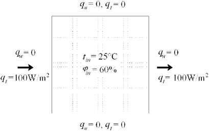
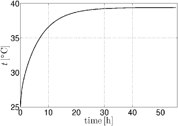
(a)	(b)

Figure 6: Example: (a) Geometry and boundary conditions, (b) Evolution of temperature at $\mbox{\boldmath$x$}^{0}$

Parameter	Mortar	Sandstone
density [kgm-3]	1700	1964
specific heat $c$ [Jkg-1K-1]	1000	900
vapor diffusion resistance number $\mu$, see Eq. (44)	12	10

Table 3: Constant material parameters of individual phases

The constant material parameters are listed in Table 3. The moisture dependent variation of phase thermal conductivities and liquid diffusivities is plotted in Fig. 7 together with sorption isotherms obtained from the following approximations [7]

$$w = \left(1-\sqrt{1-\varphi}\right)\frac{w_{hyg}}{1-\sqrt{1-\varphi_{hyg}}},$$ (40)

$$w = w_{hyg}+\frac{\varphi-\varphi_{hyg}}{1-\varphi_{hyg}}\left(w_{sat}-w_{hyg}\right),$$ (41)

where the saturation moisture content $w_{sat}$ = 0.3, the hygroscopic moisture content $w_{hyg}$ = 0.02 and the hygroscopic relative humidity $\varphi_{hyg}$ = 95$\%$ were assumed.

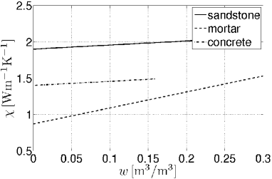
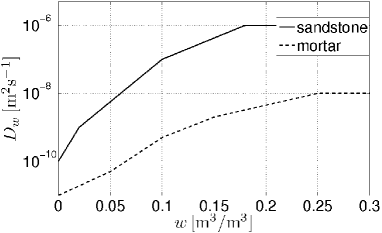
(a)	(b)

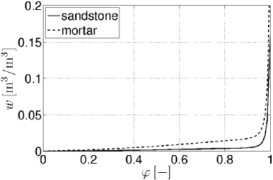
(c)

Figure 7: Example - material data: (a) variation of phase thermal conductivities as a function of volume moisture, (b) variation of phase liquid diffusivities as a function of volume moisture, (c) phase sorption isotherms

The remaining parameters that enter Eqs. (31) - (35) are provided by

• $h_{v}$ specific heat of evaporation [Jkg^-1]

  $$h_{v}=2.5008\cdot{}10^{6}\left(\frac{273.15}{t}\right)^{(0.167+t\cdot{}3.67\cdot{}10^{-4})}.$$ (42)

• $p_{\rm sat}$ saturation vapor pressure [Pa], see [11]

  $$p_{\rm sat}={\rm exp}\left(23.5771-\frac{4042.9}{t-37.58}\right).$$ (43)

• $\delta_{p}$ vapor permeability of the porous material [kgm^-1s^-1Pa^-1]

  $$\delta_{p}=\frac{\delta}{\mu},$$ (44)

  where $\mu$ is the vapor diffusion resistance number and $\delta$ is the vapor diffusion coefficient in air [kgm^-1s^-1Pa^-1] given by, see [20]

  $$\delta=\frac{2.306\cdot{}10^{-5}\cdot p_{a}}{R_{v}\cdot t\cdot p}\left(\frac{t}{273.15}\right)^{1.81},$$ (45)

  with $p$ set equal to atmospheric pressure $p_{a}$ = 101325 Pa and $R_{v}$ = $R$/$M_{w}$ = 461.5; $R$ is the gas constant (8314.41 Jkmol^-1K^-1) and $M_{w}$ is the molar mass of water (18.01528 kgmol^-1).

The total temperature field $t=T+t^{*}$, which corresponds to $q_{x}=\mathrm{100Wm^{-2}}$, appears in Fig. 8(a). In this case the room initial temperature $t_{in}=25^{\circ}\mathrm{C}$ and relative humidity $\varphi=60\%$ were considered, recall Fig. 6(a). As evident from Fig. 8(b), the volume moisture field $w\,\mathrm{(m^{3}/m^{3})}$ considerably varies throughout the RVE thus affecting the macroscopic thermal conductivity slightly depending on the size of the RVE.

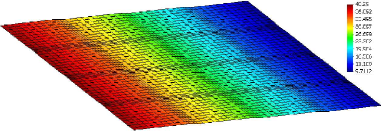
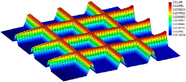
(a)	(b)

Figure 8: Example: (a) Distribution of temperature (b) Distribution of volume moisture

Several interesting results have been derived within the scope of our numerical experiments. The graph in Fig. 9(a) displays the dependence of the macroscopic heat conductivity $\chi^{hom}$ on the average relative humidity $\varphi$. Individual values of $\chi^{hom}$ follow again from Eq. (27). Note that this equation corresponds to steady state conditions attained after running the transient heat conduction problem for about 50 hours, see Fig. 6(b) showing an evolution of temperature at a reference point $\mbox{\boldmath$x$}^{0}$ with respect to time. It should be pointed out that the nearly linear dependence between these two variables at a sub-hygroscopic region (up to about 95% - 98%) becomes highly non-linear once the hygroscopic moisture is attained and approaches the capillary and even maximum (vacuum) saturation. Fig. 9(b) displays the relation between the macroscopic thermal conductivity and the initial temperature for different levels of the relative humidity $\varphi_{in}$.

These information were subsequently utilized when performing the analysis of Charles Bridge. It has been observed experimentally that different sections of the bridge experience different moisture content. The results in Fig. 9 thus allowed us to assign to each measured value $\varphi$ the corresponding value of $\chi^{hom}$ in the macroscopic steady state analysis of Charles Bridge. This then provided the space distribution of temperature eventually used in the thermo-mechanical analysis of the bridge [17].

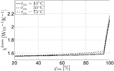
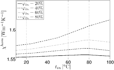
(a)	(b)

Figure 9: Example - evolution of $\chi^{hom}$ as a function of: (a) $\varphi$ at $t_{in}=25^{\circ}\mathrm{C}$, (b) $t_{in}$

The sensitivity of effective thermal conductivities on the variation of macroscopic temperature gradient was also studied. Clearly, the results presented in Fig. 10 suggest that the coefficient of the macroscopic thermal conductivity $\chi^{hom}$ is almost insensitive to the changes in the macroscopic temperature gradient $T_{,i}$, which considerably simplifies the micro (meso)-macro approach.

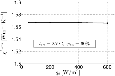
Figure 10: Example: sensitivity of $\chi^{hom}$ on variation of $T_{,i}$

5 Conclusions

Homogenization techniques applied to a meso-scale provide the values of effective transport parameters, such as the coefficient of thermal conductivity (and/or moisture permeability), and allow for their dependence on both macroscopic temperature and moisture fields. As efficient tools, the SIFEL and DELPHIN computer codes can be effectively used when analyzing transport processes within a certain PUC to get distributions of these fields on a meso-scale, while taking into account the coupling effects in transport phenomena. With reference to thermal conductivity the following conclusions can be pointed out:

• At low levels of moisture the coefficient of thermal conductivity varies almost linearly with the relative humidity $\varphi$. This relation becomes strongly non-linear as soon as the hygroscopic moisture $(\varphi\approx 95\%)$ is attained.

• The macroscopic volume moisture $(\mathrm{m}^{3}/\mathrm{m}^{3})$ extensively varies throughout the RVE thus affecting the value of macroscopic thermal conductivity.

• There exists a certain dependence of the macroscopic thermal conductivity on the initial temperature $t_{in}$. But it is distinctive just at higher temperatures, say above $30^{\circ}\mathrm{C}$.

• A very important finding is that the macroscopic conductivity is nearly insensitive to the macroscopic temperature gradient, even in the non-linear range, which simplifies the meso-macro approach.

Finally recall a relatively good correspondence between the numerically obtained values of the effective conductivities and those calculated from simple rules of mixture, see Table 2. It should be, however, mentioned that such a good agreement is merely attributed to the selected geometrical arrangement of the two phases. When more realistic periodic unit cells (such as the one displayed in Fig. 11) were used, the simple bounds were too far apart to be of any practical use.

Colour image		Binary image		SEPUC
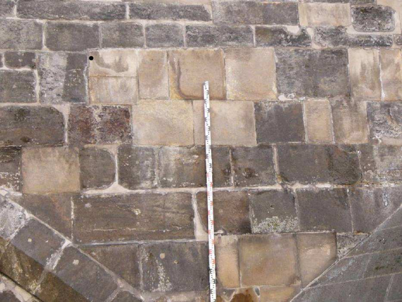
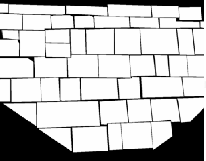
	$\mathbf{\Rightarrow}$		$\mathbf{\Rightarrow}$

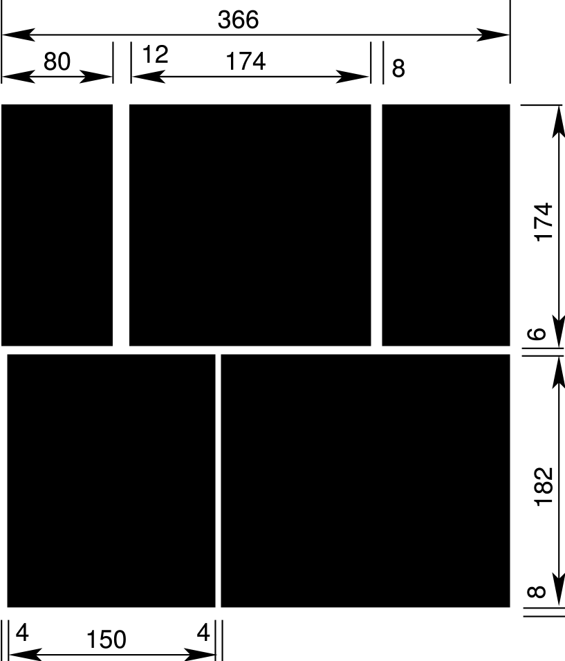
Figure 11: Construction of statistically equivalent periodic unit cell (SEPUC) for random-coursed masonry [25]

References

- [1] J.L. Auriault, Effective macroscopic description for heat conduction in periodic composites, International Journal of Heat Mass Transfer 26 (1983), 861–869.
- [2] M.A. Biot, General theory of three-dimensional consolidation, J. Appl. Phys. 12 (1941), 155–164.
- [3] Z. Bittnar and Šejnoha J., Numerical methods in structural engineering, ASCE Press, 1996.
- [4] C. Boutin, Microstructural influence on heat conduction, International Journal of Heat Mass Transfer 38 (1995), 3181–3195.
- [5] R. De Boer, Highlights in the historical development of the porous media theory: toward a consistent macroscopic theory, Applied Mechanical Review 49 (1996), 201–262, Submitted.
- [6] J. Grunewald, Diffusiver und konvektiver stoff- und energietransport in kapillarpor sen baustoffen, Ph.D. thesis, TU Dresden, 1997.
- [7] J. Grunewald, Delphin 4.1 documentation, theoretical fundamentals, Dresden:, TU Dresden, 2000.
- [8] M. Hassanizadech and W.G. Gray, General conservation equations for multiphase systems: 1, averaging procedure, Adv. Water Resources 2 (1979), 131–144.
- [9] M. Hassanizadech and W.G. Gray, General conservation equations for multiphase systems: 2, mass, momenta, energy and entropy equations, Adv. Water Resources 2 (1979), 191–203.
- [10] M. Kaminski, Homogenization of transient heat transfer problems for some composite materials, International Journal of Engineering Science 41 (2003), 1–29.
- [11] T. Krejčí, T. Nový, L. Sehnoutek, and J. Šejnoha, Structure - subsoil interaction in view of transport processes in porous media, CTU Reports, vol. 5, CTU in Prague, 2001, 81 pp.
- [12] O. Krischer, Die wissentschaftliche grundlagen der trocknugstechnik, 2. auflage ed., Berlin:Springer Verlag, 1963.
- [13] J. Kruis, T. Krejčí, and Z. Bittnar, Numerical solution of coupled problems, Proceedings of The Ninth International Conference on Civil and Structural Engineering Computing (B.H.V. Topping, ed.), Civil-Comp Press, 2003, on CD ROM.
- [14] H.M. Künzel and K. Kiessl, Calculation of heat and moisture transfer in exposed building components, International Journal of Heat Mass Transfer 40 (1997), 159–167.
- [15] Malvern L.E., Introduction to the mechanics of a continuous medium, Prentice-Hall, Inc., Englewood Cliffs, N.J., 1969.
- [16] R. W. Lewis and B. A. Schrefler, The finite element method in the static and dynamic deformation and consolidation of porous media, John Wiley&Sons, Chichester, England, 2nd edition, 1999.
- [17] J. Novák, J. Zeman, M. Šejnoha, and J. Šejnoha, Pragmatic multi-scale and multi-physics analysis of charles bridge in prague, submitted, (2007), http://mech.fsv.cvut.cz/~zemanj/preprints/engstruct_08_ZeNoSeSe.pdf
- [18] I. Oezdemir, W. A. M. Brekelmans, and M. G. D. Geers, Computational homogenization for heat conduction in heterogeneous solids, International journal for numerical methods in engineering 0 (2006), 0–0, Article in press, http://dx.doi.org/10.1002/nme.2068.
- [19] J.R. Philip and D.A. de Vries, Moisture movement in porous materials under temperature gradients, Transaction of the American Geophysical Union 38 (1957), 222–232.
- [20] R Schirmer, Zvdi, Beiheft Verfahrenstechnik 6 (1938), 170.
- [21] J. Sýkora, J. Vorel, J. Šejnoha, and M. Šejnoha, Effective material parameters for transport processes in historical masonry structures, Proceedings of the Tenth International Conference on Civil, Structural and Environmental Engineering Computing (Stirling, United Kingdom) (B. H. V. Topping, ed.), Civil-Comp Press, 2005, paper 190.
- [22] B. Tomková, M. Šejnoha, J. Novák, and J. Zeman, Evaluation of effective thermal conductivities of porous textile composites (2008) submitted, 0803.3028
- [23] R. Černý and P. Rovnaníková, Transport processes in concrete, London: Spon Press, 2002.
- [24] J. Šejnoha, J. Zeman, J. Novák, and Z. Janda, Non-linear three-dimensional analysis of the charles bridge exposed to temperature impact, Proceedings of the Tenth International Conference on Civil, Structural and Environmental Engineering Computing (Stirling, United Kingdom) (B. H. V. Topping, ed.), Civil-Comp Press, 2005, paper 187.
- [25] J. Zeman and M. Šejnoha, From random microstructures to representative volume elements, Modelling and Simulation in Materials Science and Engineering 15 (2007), no. 4, S325–S335.