Generating derivative structures: Algorithm and applications

Abstract

We present an algorithm for generating all derivative superstructures—for arbitrary parent structures and for any number of atom types. This algorithm enumerates superlattices and atomic configurations in a geometry-independent way. The key concept is to use the quotient group associated with each superlattice to determine all unique atomic configurations. The run time of the algorithm scales linearly with the number of unique structures found. We show several applications demonstrating how the algorithm can be used in materials design problems. We predict an altogether new crystal structure in Cd-Pt and Pd-Pt, and several new ground states in Pd-rich and Pt-rich binary systems.

I Why derivative structures?

Derivative superstructuresBuerger (1947) play an important role in different materials phenomenon such as chemical ordering in alloys, spin ordering in magnets, and vacancy ordering in non-stoichiometric materials. Similarly, derivative superlatticesnot (a); Santoro and Mighell (1973, 1972) are important in problems such as twinning. What is a derivative superstructure? A derivative superstructure is a structure whose lattice vectors are multiples of those of a ‘parent lattice’ and whose atomic basis vectors correspond to lattice points of the parent lattice. Many structures of intermetallic compounds can be classified as fcc-derived superstructures. These superstructures have atomic sites that closely correspond to the sites of an fcc lattice but some of the translational symmetry is broken by a periodic arrangement of different kinds of atoms. The structures shown in Fig. 2 comprise the set of all fcc-derived binary superstructures with unit cell sizes 2, 3, and 4 times larger than the parent lattice.

Large sets of derivative superstructures are often used in (practically) exhaustive searches of binary configurations on a lattice to determine ground state properties of intermetallic systems. The approach is not limited to searches of configurational energies, but other physical observables can also be targeted if an appropriate Hamiltonian is available. For example, Kim et al.Kim et al. (2005) used an empirical pseudopotential Hamiltonian and a large list of derivative superstructures to directly search semiconductor alloys for desirable band-gaps and effective masses. The set of derivative superstructures is useful in any situation where the physical observable of interest depends on the atomic configuration.

For the aforementioned reasons, an algorithm for systematically generating all superstructures of a given parent structure is useful. Such an algorithm has been presented in the literature only onceFerreira et al. (1991) (FWZ below), but closely related algorithms have been implemented in several alloy modeling packages.van de Walle and Ceder (2002); van de Walle et al. (2002); Zarkevich et al. (2007) The FWZ algorithm is restricted to fcc- and bcc-based superstructures and to binary cases only. Furthermore, the list generated by the FWZ algorithm is formally incomplete (though in practice it may be sufficient).not (b)

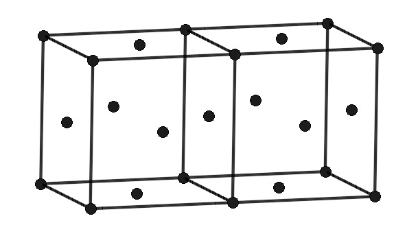
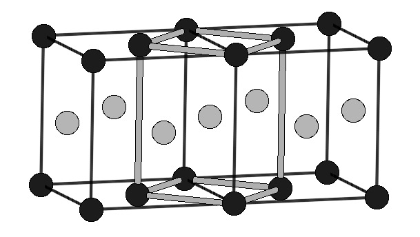
Figure 1: An example parent lattice (left) and a superstructure (right). The parent lattice is fcc and the superlattice is defined by the (doubled) unit cell outlined in gray. The two interior points of the superlattice are occupied by one black atom and one gray atom. The superlattice + atoms constitute a derivative structure. The superstructure of this example is that of CuAu.

The purpose of this paper is to present a general algorithm that generates a formally complete list of two- or three-dimensional superstructures, and that works for any parent lattice and for arbitrary $k$-nary systems (binary, ternary, etc.). This algorithm is conceptually distinct from FWZ and related implementations. Instead of using a geometrical, ‘smallest first’ approach to the enumeration,Zarkevich et al. (2007) it takes advantage of known group theoretical properties of integer matrices. The algorithm is orders of magnitude faster than FWZ, more general, and formally complete. A Fortran 95 implementation of the algorithm is included with this paper as supplementary material.

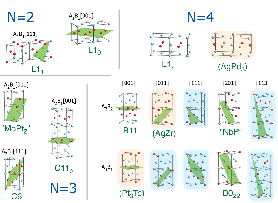
Figure 2: The first 17 binary structures derived from the fcc lattice. All have 4 atoms/cell or less. Structures shown with a green plane can be characterized as a stacking of pure A and B atomic layers. For example the L1₀ structure (upper left) is an alternating (A₁B₁) sequence of layers stacked in the [001] direction. All of the 2- and 3-atoms/cell structures have physical manifestations. Of the 4-atoms/cell structures only four have physical manifestations. Three of the others (yellow backgrounds) have been predicted to existCurtarolo et al. (2005) but not yet observed. The other five (purple backgrounds) have never been observed or predicted to exist in any system.

Mathematically, we can describe the purpose of the algorithm as this: for a given parent lattice, enumerate all possible superlattices and all rotationally- and translationally-unique ‘colorings’ or labelings of each superlattice. In presenting the algorithm in the next section, we shall refer to superlattices and labelings rather than referring to crystal structures or atomic sites.

II Enumerating all derivative structures

Here is a brief outline of the algorithm.

1. For each superlattice of size $n$, generate all Hermite Normal Form (HNF) matrices.Santoro and Mighell (1973, 1972) (In what follows, we refer to $n$ as the index of the superlattice.)

2. Use the symmetry of the parent lattice to remove rotationally-equivalent superlattices, thus shrinking the list of HNF matrices.

3. For each superlattice index $n$, find the Smith Normal Form (SNF) of each HNF in the list, and:

   1. Generate a list of possible labelings (atomic configurations) for each SNF, essentially a list of all $k^{n}$ numbers in a base $k$, $n$-digit system. For the labels, we use the first $k$ letters of the alphabet, $a,b,\cdots$.

   2. Remove incomplete labelings where each of the $k$ labels ($a,b,\cdots$) does not appear at least once.

   3. Remove labelings that are equivalent under translation of the parent lattice vectors. This reduces the list of labelings by a factor of $\approx n$.

   4. Remove labelings that are equivalent under an exchange of labels, i.e., $a\rightleftharpoons b$, so that, e.g., the labeling $aabbaa$ is removed from the list because it is equivalent to $bbaabb$.

   5. Remove labelings that are super-periodic, i.e., labelings that correspond to a non-primitive superstructure. This can be done without using the geometry of the superlattice.

4. For each HNF, remove labelings that are permuted by symmetry operations (of the parent lattice) that leave the superlattice fixed.

An important feature of the algorithm is that the the list of possible labelings, generated in step 3a, form a minimal hash table with a perfect hash function. Eliminating all duplicate labelings in a list of $N$ can be accomplished in $O(N)$ time. Coupled with the group theoretical approach, this results in an extremely efficient algorithm, orders of magnitude faster than FWZ, and which scales linearly. That is, the time to find $N$ unique structures scales linearly with $N$, regardless of the size of $N$. This linear scaling is shown for the case of binary superstructures of an fcc parent lattice in Fig. 3.

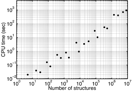
Figure 3: Required CPU time as a function of the number of unique derivative superstructures found. The scaling is linear, the best possible scaling for this type of problem.

II.1 Generating all superlattices

Given a ‘parent’ cell (any lattice), the first step in finding all derivative structures of that cell is to enumerate all derivative superlattices. Consider the transformation $\mathbb{B=AH}$ where $\mathbb{A}$ is the basis for the original lattice (the basis vectors listed column-wise), $\mathbb{H}$ is a matrix with all integer elements, and $\mathbb{B}$ is the matrix of the transformed lattice. If the determinant of the transformation matrix, $|\mathbb{H}|$, is $\pm 1$, then $\mathbb{H}$ is merely a change of basis that leaves the lattice represented by $\mathbb{A}$ unchanged. Matrices $\mathbb{A}$ and $\mathbb{B}$ are merely two different choices of basis for the same lattice. On the other hand, if the elements of $\mathbb{H}$ are all integers but the determinant of $\mathbb{H}$ is 2, say, then the lattice of $\mathbb{B}$ is a superlatticeSantoro and Mighell (1972) of (i.e., a subgroup) of the lattice defined by $\mathbb{A}$, but with twice the volume of the original (parent) lattice.

Two different matrices, $\mathbb{H}_{1}$ and $\mathbb{H}_{2}$, with the same determinant, will generate different bases for the same lattice if and only if $\mathbb{H}_{1}$ can be reduced to $\mathbb{H}_{2}$ by elementary integer column operations. The canonical form for such operations is lower triangular Hermite Normal Form (HNF). Thus, if we use only matrices $\mathbb{H}$ which are in HNF, we will produce exactly one representation of each superlattice.Santoro and Mighell (1973, 1972) In three dimensions, the lower-triangular Hermite Normal Form is

$$\left(\begin{array}[]{ccc}a&0&0\\ b&c&0\\ d&e&f\\ \end{array}\right)\qquad\textrm{with}\qquad 0\leq b<c,\quad 0\leq d,e<f.$$ (1)

In this form, the product of the integers on the diagonal alone, $a\times c\times f$, fixes the determinant. Again, we refer to the superlattice size, or the determinant, as the index $n$. Generating all HNF matrices of a given index can be done then by finding each unique triplet, $acf=|\mathbb{H}|$, and then generating all values of $b$, $d$, and $e$ that obey the conditions in (1).

The algorithm for generating all possible HNF matrices of a given index $|\mathbb{H}|$ is rather simple, comprising just two steps. In the first step, find all possible diagonals: find all values $a$, $1\leq a\leq|\mathbb{H}|$, that evenly divide $|\mathbb{H}|$; for each of these values, find all $c$, $1\leq c\leq|\mathbb{H}|/a$, that evenly divide $|\mathbb{H}|/a$. For each value of $c$, let $f=|\mathbb{H}|/(ac)$. For example, consider the case of $|\mathbb{H}|=6$. We execute two nested loops over the possible values of $a$ and $c$; each loop runs over all integers between 1 and the $|\mathbb{H}|$, testing the above conditions at each iteration. The loops run from 1 to 6, and the algorithm finds eight cases that meet the above conditions. They are:

$$\begin{array}[]{c|cccccccc}a&1&1&1&2&2&3&3&6\\ \hline\cr c&1&2&3&1&3&1&2&1\\ \hline\cr f&6&3&2&3&1&2&1&1\\ \end{array}$$

The set of $acf$ triplets generated during this first step comprises all possible diagonals of the HNF matrices for the case of $n=|\mathbb{H}|=6$. The second step, generating each set of values of $b$, $d$, and $e$ for each diagonal (set of $acf$ triplets), can be accomplished simply by three nested loops that start at zero and terminate at $b<c$ and $d,e<f$.

As an example of both steps, consider the case where the index is merely double that of the original lattice, i.e., where $|\mathbb{H}|=2$. The factors of 2 are just the set $\{1,2\}$, so the first step finds only three cases: (2,1,1), (1,2,1), and (1,1,2). Then, generating the off-diagonal terms for each of these three cases, we find seven HNF matrices:

$$\begin{array}[]{cccccc}\textrm{case 1:}&\left(\begin{array}[]{ccc}2&0&0\\ 0&1&0\\ 0&0&1\\ \end{array}\right)&&\textrm{case 2:}&\left(\begin{array}[]{ccc}1&0&0\\ 0&2&0\\ 0&0&1\\ \end{array}\right)&\left(\begin{array}[]{ccc}1&0&0\\ 1&2&0\\ 0&0&1\\ \end{array}\right)\\ \end{array}\\$$

$$\begin{array}[]{ccccc}\textrm{case 3:}&\left(\begin{array}[]{ccc}1&0&0\\ 0&1&0\\ 0&0&2\\ \end{array}\right)&\left(\begin{array}[]{ccc}1&0&0\\ 0&1&0\\ 0&1&2\\ \end{array}\right)&\left(\begin{array}[]{ccc}1&0&0\\ 0&1&0\\ 1&0&2\\ \end{array}\right)&\left(\begin{array}[]{ccc}1&0&0\\ 0&1&0\\ 1&1&2\\ \end{array}\right)\\ \end{array}$$

For increasing index, $n=|\mathbb{H}|=1,2,3,\cdots$, the number of HNF matrices generates an interesting sequence: 1, 7, 13, 35, 31, 91, $\cdots$. This sequence appears in Sloane’s databaseSloane (a) as A001001. The closed-form expression for $n$-th term in the series is

$$\sum_{d\big{|}n}d\>\sigma(d)=\prod_{i=1}^{k}\left(\frac{(p_{i}^{e_{i}+2}-1)(p_{i}^{e_{i}+1}-1)}{(p_{i}-1)^{2}(p_{i}+1)}\right),$$ (2)

where $\sigma$ is the sum of divisors function, and where the $p_{i}$ and $e_{i}$ are the prime factors and powers of $n$: $n=p_{1}^{e_{1}}\cdot p_{2}^{e_{2}}\cdots p_{k}^{e_{k}}$. The sequence appears in the crystallography literatureRutherford (1992); Billiet and Le Coz (1980) as well as several other contexts.Liskovets and Mednykh (2000); Baake (1997); Stanley (1999); Sloane (b)

Significantly, because we have an expression for the number of superlattices, the implementation of the HNF-generating algorithm can be rigorously checked. Also note that this step of the algorithm is independent of the choice of parent lattice.

II.2 Reducing HNF list by parent lattice symmetry

The set of HNF matrices defines the set of all derivative superlattices of a parent cell via the transformation mentioned above, $\mathbb{B=AH}$. However, not all of the superlattices in this set will be geometrically different. Some distinct lattices will be equivalent under symmetries of the parent lattice, illustrated in the example below.

Such duplicate superstructures must be eliminated by the algorithm. At the end of the algorithm we want all derivative structures to be unique from a materials point of view. So we wish to exclude from the list any superstructures that are related to others already in the list simply by a rotation, reflection or change of basis.

As an illustration, consider a two-dimensional parent lattice that is square, that is, $\mathbb{A=I}$ (the two-by-two identity matrix). There are three HNF matrices for which $|\mathbb{H}|=2$ and three corresponding superlattices, $\mathbb{B=AH=IH=H}$:

$$\left(\begin{array}[]{cc}2&0\\ 0&1\\ \end{array}\right)$$

$$\left(\begin{array}[]{cc}1&0\\ 0&2\\ \end{array}\right)$$

$$\left(\begin{array}[]{cc}1&0\\ 1&2\\ \end{array}\right)$$

The parent lattice itself is indicated by dots (filled and unfilled) while the superlattice is indicated by filled dots. The vectors defined by the matrices are shown as arrows. The first two lattices are clearly equivalent under a 90^∘ rotation, one of the eight symmetry operations of a square lattice.

To enumerate the distinct superlattices of a given index $n$ then, we must check that each new superlattice that is added to the list is not a rotated duplicate of a previous superlattice. More precisely, we must check that each new basis $\mathbb{B}_{i}$ is not equivalent, under change-of-basis, to some symmetric image $\mathbb{RB}_{j}$ of a basis $\mathbb{B}_{j}$ already in the list. In other words, we want to avoid the relation $\mathbb{B}_{i}=\mathbb{RB}_{j}\mathbb{H}$ where $\mathbb{B}_{i}$ is a candidate superlattice, $\mathbb{R}$ is any of the rotations of the parent lattice, $\mathbb{B}_{j}$ is a superlattice already in the list of distinct superlattices, and $\mathbb{H}$ is any unimodular matrix of integers. (Since $\mathbb{B}_{i}$ and $\mathbb{B}_{j}$ have the same determinant, we will only need to check that $\mathbb{B}_{j}^{-1}\mathbb{R}^{-1}\mathbb{B}_{i}$ is a matrix of integers.)

For the case of cubic symmetry, the seven superlattices for the $\mathbb{H}=2$ case mentioned above reduce to only two symmetrically-distinct superlattices. The corresponding derivative superstructures are L1₀ and L1₁, both well-known structures in intermetallic compounds. The fact that these are the only two 2-atom/cell fcc structures is not coincidence or an accident of chemistry; no other 2-atom/cell structures are possible geometrically. The hierarchy of physically-observed structures uncovered for fcc and bcc lattices as the index is increased is discussed in Refs. Hart, 2007a, b. Additional applications can be found in Sec. IV.

II.3 Find the unique labelings for all superlattices

II.3.1 Generate all possible labelings

For each HNF, each superlattice, we start by generating all possible labelings of that superlattice. In other words, given $k$ colors (types of atoms), represented by the labels $a,b,\cdots$, we generate all possible ways of labeling (coloring) the superlattice. Each HNF matrix of determinant size $n$ represents a superlattice with $n$ interior points to be decorated. If the number of colors is $k$, then the list of all possible labelings is easily represented by the list of all $n$-digit, base-$k$ numbers. So, from a combinatorial point of view, there are $k^{n}$ distinct labelings. For example, in the case of a binary system ($k=2$) with 4 interior points (index $n=4$), there are $2^{4}=16$ possible labelings (see Table 1).

$$\begin{array}[]{cccc}\hbox{\pagecolor{incomplete}aaaa}&\hbox{\pagecolor{transdup}abaa}&\hbox{\pagecolor{transdup}baaa}&\hbox{\pagecolor{transdup}bbaa}\\ aaab&\hbox{\pagecolor{nonprim}abab}&\hbox{\pagecolor{transdup}baab}&\hbox{\pagecolor{labperm}bbab}\\ \hbox{\pagecolor{transdup}aaba}&\hbox{\pagecolor{transdup}abba}&\hbox{\pagecolor{transdup}baba}&\hbox{\pagecolor{labperm}bbba}\\ aabb&\hbox{\pagecolor{labperm}abbb}&\hbox{\pagecolor{labperm}babb}&\hbox{\pagecolor{incomplete}bbbb}\\ \end{array}$$

Table 1: An example labeling for the binary case, $k=2$, with 4 interior points, $n=4$, in the superlattice. There are $k^{n}=2^{4}=16$ distinct labelings, but the colored labelings represent incomplete or duplicate superstructures. Yellow labelings are incomplete (not all labels are present), purple are translation duplicates, blue are label-exchange duplicates, and green are super-periodic labelings.

II.3.2 Concept of eliminating duplicate labelings

The rest of the algorithm deals with just one conceptual issue—given the $k^{n}$ labelings/colorings of the superlattice, eliminate the duplicates. In the FWZ algorithm and its extended implementations, duplicate structures are eliminated by directly comparingnot (c) one candidate structure to another geometrically, necessitating an expensive $O(N^{2})$ search. We eliminate the duplicates via group theory rather than checking the structures themselves. Although this approach is more abstract than the geometric approach, it is much more efficient—eliminating the duplicates in a list becomes a strictly $O(N)$ procedure.

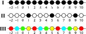
Figure 4: (I) One-dimensional example of a parent lattice, (II) a derivative superlattice (index $n=4$), (III) one possible superlattice labeling.

One-dimensional example: We start with a simple illustration and then discuss the essential group theoretical concepts in the context of that example. Consider the one-dimensional case of Fig. 4. The first line (I) is a parent lattice, an infinite collection of equally-spaced points, identified with the set of integers, denoted ${\bf Z}$. The second line (II) is a superlattice, a subset of the parent lattice (every fourth point; those colored black). The third line (III) is a superstructure, a ‘labeling’ or ‘coloring’ of the parent lattice that has the same periodicity as the superlattice. The points of the lattice play the role of positions in a crystal, and the colors/labels play the role of atoms placed at those positions.

There are labelings that are distinct yet physically equivalent, as shown in Fig. 5. Note that line (II) is obtained from line (I) by shifting the colors two units to the right, and line (III) is obtained from line (I) by shifting the numbers two units to the left—with the same result. Lines (II) and (III) are the same labeling, obtained in different ways from (I). Both are physically equivalent to (I). The fact that we can obtain such a shifted labeling either by shifting the numbers or by shifting the labels explains why we can do much of our equivalence checking within a finite group, instead of geometrically within an infinite lattice. By this method, we will identify these equivalent labelings and remove them from the original list of $k^{n}$ labelings.

We may illustrate the group theory approach using Fig. 4. The parent lattice (I) is the set of integers ${\bf Z}$, which is a group under the addition operation. We refer to this group as $L$. The superlattice is the set of multiples of 4, denoted $4{\bf Z}$. We refer to this subgroup of $L$ as $S$. We label the parent lattice $L$ in a manner which is periodic with respect to the superlattice $S$, and note that if two points differ by an element of the superlattice, they must receive the same label. We use colors as labels in line (III) of Fig. 4 and note that every fourth point has the same color.

Notice that the green points are our superlattice are $4{\bf Z}$, and the yellow points are a copy of $4{\bf Z}$, but translated one unit to the right. Thus, we may denote the latter set (the yellow points) by the set $1+4{\bf Z}$. Similarly, the red points are the set $2+4{\bf Z}$, and the blue points are $3+4{\bf Z}$. These four sets, $4{\bf Z},\,1+4{\bf Z},\,2+4{\bf Z},\,3+4{\bf Z}$, are mutually disjoint (they don’t overlap), and their union is the entire parent lattice $L$. They are translations of $S$; and thus are the cosets of the subgroup $S$. This means we can use them to form a new group, called the quotient group $G=L/S$ (see Table 2). This new group is finite, having only four elements. For notational convenience we shall also refer to these 4 elements of $G$ as (0,1,2,3). We need only label the four elements of our quotient group in order to label the entire parent lattice.

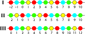
Figure 5: Three labelings of the superlattice of Fig. 4. Lines II and III are identical to line I except the colors (labels) are shifted. In line II the colors have been shifted two units to the right. In line III, the shift has been effected by translating the lattice two units to the left.

Suppose we wish to translate a labeling (in order to identify and eliminate equivalent structures). As shown in line (I) of Fig. 5 we have labeled the elements of the quotient group as follows (using $g$, $y$, $r$ and $b$ for the colors):

$$\begin{array}[]{lccc}0:&\quad 4{\bf Z}&\rightarrow&g\\ 1:&\quad 1+4{\bf Z}&\rightarrow&y\\ 2:&\quad 2+4{\bf Z}&\rightarrow&r\\ 3:&\quad 3+4{\bf Z}&\rightarrow&b.\end{array}$$

In Fig. 5, we see that translating the labels by two is the same as simply adding 2 to each coordinate, thus:

$$\begin{array}[]{rcl}4{\bf Z}&\rightarrow&2+4{\bf Z}\\ 1+4{\bf Z}&\rightarrow&3+4{\bf Z}\\ 2+4{\bf Z}&\rightarrow&4+4{\bf Z}=4{\bf Z}\\ 3+4{\bf Z}&\rightarrow&5+4{\bf Z}=1+4{\bf Z}\end{array}\qquad\begin{array}[]{rcl}0&\rightarrow&2\\ 1&\rightarrow&3\\ 2&\rightarrow&0\\ 3&\rightarrow&1\\ \end{array}$$

The effect is the same as if we had assigned the colors differently:

$$\begin{array}[]{lccc}0:&\quad 4{\bf Z}&\rightarrow&r\\ 1:&\quad 1+4{\bf Z}&\rightarrow&b\\ 2:&\quad 2+4{\bf Z}&\rightarrow&g\\ 3:&\quad 3+4{\bf Z}&\rightarrow&y.\end{array}$$

Translating the lattice by adding $+2$ to every point (moving the origin by 2 units) has the same effect on the labeling as if we had merely labeled the four elements of the quotient group, and then added $+2$ to every element of the group, producing the permutation $0\rightarrow 2$, $1\rightarrow 3$, $2\rightarrow 0$ and $3\rightarrow 1$, denoted (2,0,3,1).

	$\mathbf{Z}$	$1+\mathbf{Z}$	$2+\mathbf{Z}$	$3+\mathbf{Z}$
$\mathbf{Z}$	$\mathbf{Z}$	$1+\mathbf{Z}$	$2+\mathbf{Z}$	$3+\mathbf{Z}$
$1+\mathbf{Z}$	$1+\mathbf{Z}$	$2+\mathbf{Z}$	$3+\mathbf{Z}$	$\mathbf{Z}$
$2+\mathbf{Z}$	$2+\mathbf{Z}$	$3+\mathbf{Z}$	$\mathbf{Z}$	$1+\mathbf{Z}$
$3+\mathbf{Z}$	$3+\mathbf{Z}$	$\mathbf{Z}$	$1+\mathbf{Z}$	$2+\mathbf{Z}$

	$0$	$1$	$2$	$3$
$0$	$0$	$1$	$2$	$3$
$1$	$1$	$2$	$3$	$0$
$2$	$2$	$3$	$0$	$1$
$3$	$3$	$0$	$1$	$2$

Table 2: Two representations of the Cayley table for the quotient group $G$ (cosets of the subgroup $S$). On the right, the elements of the group have been denoted (0,1,2,3) for notational convenience.

Instead of determining that two labelings of the (infinite) lattice are equivalent by translation, we may simply check that the corresponding labelings of our finite quotient group $G={\bf Z}_{4}$ are equivalent. We do this by just adding a fixed element to every element in the group, effecting a permutation of the cyclic group ${\bf Z}_{4}$. This idea—of labeling the quotient group instead of the lattice elements, and checking equivalence within the group instead of by translating the lattice—may seem unduly abstract and unnecessary in one dimension, but it becomes much more efficient and crucial in higher dimensions, as we now show.

Application to higher dimensions: In any dimension, we have a parent lattice $L$, and a superlattice $S$ which is a subgroup of $L$. Labeling $L$ in a manner which is periodic with respect to $S$ is equivalent to merely labeling the elements of the quotient group $G=L/S$. Note that even though $L$ and $S$ are infinite sets, their quotient group is always a finite group with the same number of elements as the superlattice index $n$. Again, we check for equivalence by doing operations within the group instead of by lattice translation.

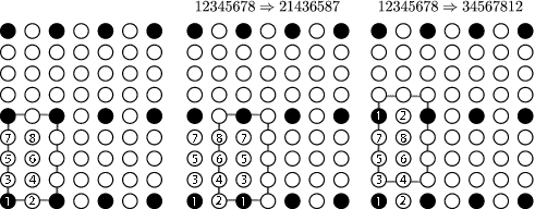
Figure 6: A superlattice whose SNF is non-trivial (non-cyclic). Because the quotient group of the superlattice is non-cyclic, translations of the lattice are not cyclic permutations. Instead the sites are permuted in groups of two or four with each translation (rather than permuting as a single group of 8). In the figure, three different pictures of the same superlattice are shown. In each case a different origin is chosen. In the second case, the translation permutes two groups of 4 sites, in the third, 4 pairs are permuted.

The key to this approach is the Smith normal form (SNF). The SNF is useful because it provides the quotient group directly as follows. Recall that if $\mathbb{A}$ is a basis for $L$, then the distinct lattices of index $n$ are uniquely characterized by bases $\mathbb{B=AH}$, where $\mathbb{H}$ is a matrix of determinant $n$ in HNF. If $S$ is given by one such basis $\mathbb{B}_{1}=\mathbb{AH}_{1}$, then the quotient group $G=L/S$ can be found by converting the matrix $\mathbb{H}_{1}$ into SNF (which is a diagonal matrix with certain special properties; see Appendix). In higher dimensions the quotient group may not be purely cyclic, but it is a direct sum of cyclic groups which are given by the diagonal entries in the SNF matrix (see Fig. 6). For example if the SNF matrix is $\begin{pmatrix}2&0\\ 0&4\\ \end{pmatrix}$, then the quotient group $G=L/S$ is the direct sum ${\bf Z}_{2}\oplus{\bf Z}_{4}$.

In relation to the algorithm, there are two important facts to note about the SNF. (i) The SNF provides the quotient group directly, which in turn is the key to implementing an $O(N)$ algorithm. (ii) The number of SNFs (and so quotient groups) is small compared to the number of distinct lattices of index $n$ (see Table 3). This means that translation duplicates can be removed from the $k^{n}$ list for hundreds or thousands of different superlattices simultaneously. (The surprising geometric implications of this are discussed in the appendix.) This reduces the running time by many orders of magnitude.

$n$	2	3	4	5	6	7	8	9	10	11	12	13	14	15	16
HNFs	7	13	35	31	91	57	155	130	217	133	455	183	399	403	651
SNFs	1	1	2	1	1	1	3	2	1	1	2	1	1	1	4

Table 3: Table showing the number of Hermite normal form (HNF) matrices and Smith normal form (SNF) matrices as a function of index $n$ (determinant size). The number of HNFs is a rapidly-increasing function of $n$ (see Eq. 2) whereas the number of SNFs grows very slowly.

II.3.3 Eliminating translation duplicates

Because of its periodicity, the choice of origin of a superlattice is arbitrary. A change in origin implies a permutation of the labels that nonetheless defines the same superstructure (compare lines I and III in Fig. 5). As stated previously, by examining the quotient group instead of directly comparing the structures, the duplicate labelings can be readily identified. For example, consider the case for $n=4$. Adding each member to the quotient group $\mathbf{Z}_{4}=(0,1,2,3)$ effects 4 permutations as follows:

member	mapping	permutation
0:	0$\rightarrow 0$, 1$\rightarrow 1$, 2$\rightarrow 2$, 3$\rightarrow 3$	(0,1,2,3)
1:	0$\rightarrow 1\rightarrow 2\rightarrow 3\rightarrow 0$	(1,2,3,0)
2:	0$\rightarrow 2\rightarrow 0$, 1$\rightarrow 3\rightarrow 1$	(2,0,3,1)
3:	0$\rightarrow 3\rightarrow 2\rightarrow 1\rightarrow 0$	(3,0,1,2)

If we take the 14 complete labelings of Table 1 and the three non-trivial permutations above, we find that 10 are duplicates (colored purple in Table 1):

(0,1,2,3)	(1,2,3,0)	(2,0,3,1)	(3,0,1,2)
	duplicates
aaab	aaba	abaa	baaa
aabb	abba	bbaa	baab
abab	baba	abab	baba
abbb	bbba	bbab	babb

Of the original $2^{4}=16$ labelings, two were discarded immediately because they were incomplete. Of the remaining 14, 10 are translation duplicates, leaving 4 that are translationally inequivalent (left column above).

II.3.4 Remove ‘label-exchange’ duplicates

The next step in the algorithm is to remove labelings that are equivalent under exchange of labels. Structurally, there is no difference between a superlattice whose interior points are labeled $aaab$ versus $bbba$. Although the energy of an isostructural compound with composition X₃Y₁ is different from one with composition X₁Y₃, we only wish to include one entry in our list of derivative superstructures because the full composition list can always be recovered by making all possible label exchanges (i.e., $a\rightleftharpoons b$). In the example above, four labelings were unique under translations:

aaab

aabb

abab

abbb

But the first and the fourth are equivalent by exchanging $a\leftrightharpoons b$ and applying the permutation (1,2,3,0).

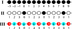
Figure 7: (color on-line) (I) One-dimensional example of a parent lattice, (II) a derivative superlattice (index $n=4$), (III) a super-periodic (or non-primitive) labeling. Although the index of the superlattice is $n=4$, the structure can be represented by a superlattice labeling of period 2 instead of 4. The superstructure of line III would have been found as an index $n=2$ derivative structure and is therefore a duplicate.

II.3.5 Remove super-periodic labelings (non-primitive structures)

At this point of the algorithm, many of the duplicate labelings have been removed from the original $k^{n}$ list. But there are still more duplicates to remove. Some of the labelings in the list will represent superstructures that are not primitive. In other words, the labelings will be super-periodic—they will have periods shorter scale than the superlattice.not (d)

The super-periodic duplicates are easily identified because they are identical under at least one permutation. The quotient group $G$ dictates a set of permutations under which the labelings are duplicate. One of these permutations will leave the labeling unchanged if it is super-periodic. For example, continuing the example above, three unique labelings are still in the list: $aaab$, $aabb$, and $abab$. One of the permutations of the quotient group $G=\mathbf{Z}_{4}$ is (2,0,3,1). Under this permutation, the labeling $abab$ is unchanged. Thus it is super-periodic, as depicted in Fig. 7. It is a duplicate in the sense that the algorithm would have already enumerated this structure with the index $n=2$ structures.

II.3.6 For each HNF: remove ‘label-rotation’ duplicates

The previous three steps of the algorithm yield a list of distinct labelings for each SNF of index $n$. Three kinds of the duplicate labelings, translation duplicates and label-exchange duplicates and super-periodic duplicates, have already been removed. One kind of duplicate remains, however, and these are eliminated in the current step.

This step removes labelings which are permuted by the rotations of the parent lattice. Whereas the preceding steps were applied to generate a list of unique labelings for each SNF, the current step must be applied to each HNF. In other words, this step must be applied to the surviving labelings separately for each superlattice.

Superlattices which are not fixed by rotations of the parent lattice were already eliminated as duplicates in step 2 of the algorithm. But rotations which leave the superlattice unchanged may still permute the labeling itself. Such permutations are physically equivalent (merely rotated with respect to one another). So any two labelings which are equivalent under rotations that fix the superlattice are duplicate and one must be removed from the list. Figure 8 illustrates the situation in two dimensions.

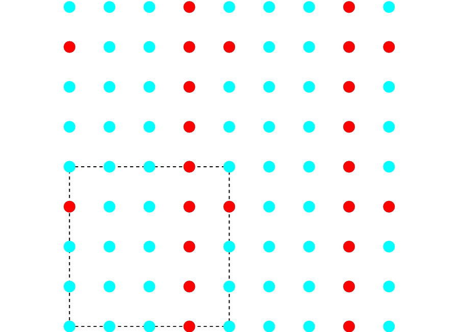
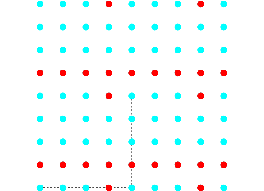
Figure 8: (color on-line) Two identical $4\times 4$ superlattices (dotted lines) with rotationally-equivalent labelings (red and blue circles). Although the superlattices themselves are unchanged, a $90^{\circ}$ rotation applied to the left labeling yields that shown on the right. Thus the second is a duplicate of the first and should be removed from the list of labelings.

Here again, the group theory approach and the SNF makes the search extremely efficient. Label rotation duplicates can be identified easily using the properties of the quotient group and the SNF transformation. The row and column operations required to transform the HNF matrix of a superlattice into its SNF can be represented by two integer transform matrices, $\mathbb{L}$ and $\mathbb{R}$, so that $\mathbb{LHR=S}$, where $\mathbb{S}$ is the SNF. This step of the algorithm is implemented using the left transformation matrix $\mathbb{L}$.

Let $\mathbb{G}$ be a $3\times n$ matrix where each member of the quotient group is represented as a columnima in $\mathbb{G}$, and let $\mathbb{R}$ be one of the rotations that fixes the superlattice. Then the permutation of the labels (which is the same as the permutations of the quotient group) enacted by the rotation $\mathbb{R}$ is given by:

$$\mathbb{G}^{\prime}=\mathbb{LA}^{-1}\mathbb{R}(\mathbb{LA}^{-1})^{-1}\mathbb{G}$$ (3)

where columns of $\mathbb{A}$ are the lattice vectors of the parent lattice, and $\mathbb{L}$ is the left transformation matrix for the SNF.

The power of this expression is that it allows the label-rotation duplicates to be identified by working entirely within the quotient group, without requiring any explicit reference to the geometry of the superlattice. Thus, as in the other steps, duplicates labelings can be eliminated in a time proportional only to the number of labelings in the list.

III Examples

In this section, we give several example derivative structure lists enumerated by the algorithm. We discuss the symmetry reduction of the structure lists and then give results for several cases. First, we compare the fcc/bcc binary list to that generated by the FWZ algorithm. We also show the small-unit-cell binary structures for a simple-cubic parent lattice and the small-unit-cell ternary structures for an fcc parent lattice.

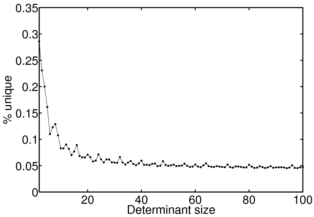
Figure 9: Symmetrically unique HNF matrices as a function of the index $n$ (determinant size) for an fcc parent lattice. Asymptotically, the fraction of unique superlattices approaches $2/N=1/24\approx 5$%, where $N=48$ is the number of symmetry operations of the fcc parent lattice.

III.1 Symmetry reduction of superlattices

In step B of the algorithm, the complete list of HNF matrices is reduced to those that are unique under the symmetry operations of the parent lattice. Asymptotically, the factor by which the list is reduced is one half the order of the rotation group of the parent lattice. For example, for cubic parent lattices (simple cubic, face-centered-, or body-centered-cubic), the point group contains 48 rotations (proper and improper). For superlattices with large index $n$, the number of HNFs is reduced by a factor of $48/2=24$. Because every lattice is symmetric under inversion, only the proper rotations (i.e., not reflections) need be considered in the reduction (thus the factor of 1/2). Figure 9 shows the fraction of symmetrically distinct superlattices for determinant sizes up to 100, while Fig. 10 shows the actual number of fcc-based superlattices compared to the total number of distinct HNF matrices.

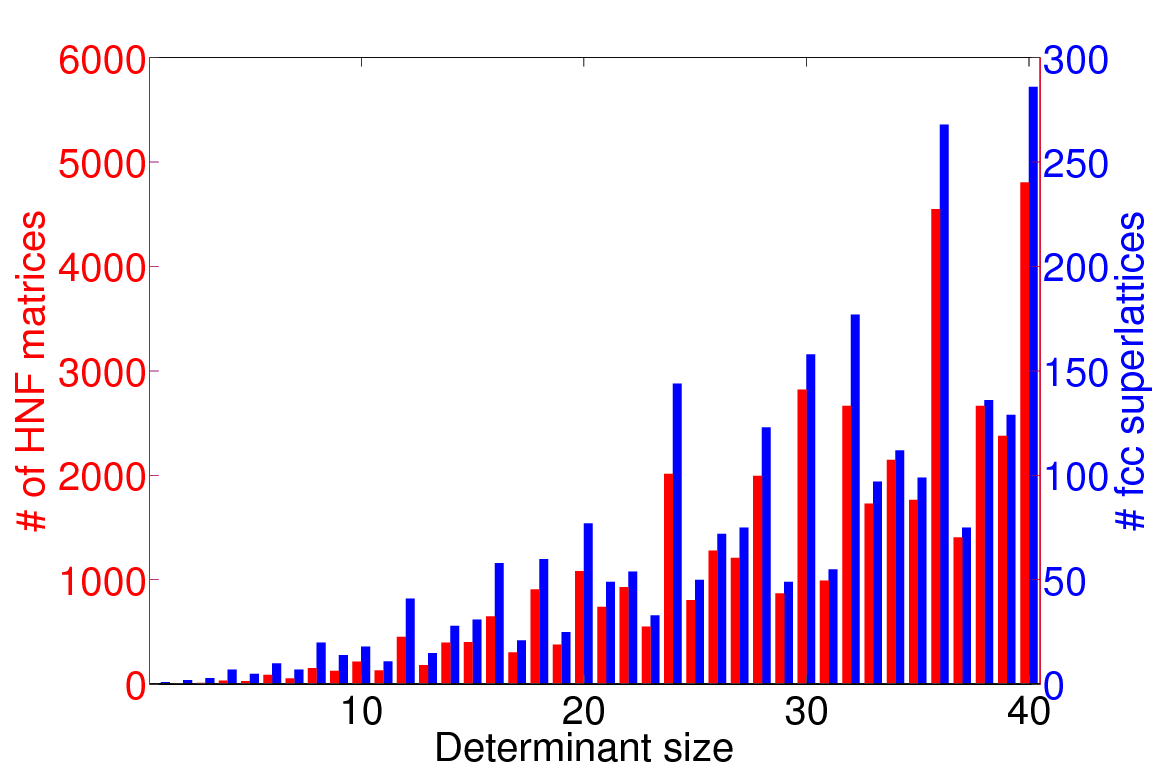
Figure 10: (color on-line) Left axis (red): Number of HNF matrices as a function of determinant size. Right axis (blue): Number of inequivalent fcc superlattices as a function of volume.

For an fcc or bcc parent lattice (the numbers are the same), the number of unique lattices as a function of index $n$ (cell size) is equivalent to the Sloane sequence A045790.Moussafir For the sequences generated for other parent lattices, which accordingly have a different symmetry group, there are no known number-theoretic connections. Surprisingly, this is even true for the simple cubic lattice. For the simple cubic lattice, the sequence is identical to the fcc/bcc one for odd values of the index $n$ but larger for the even values. (See Table 4.)

index	# of superlattices
$n$	fcc/bcc	sc	hex	tetragonal
2	2	3	3	5
3	3	3	5	5
4	7	9	11	17
5	5	5	7	9
6	10	13	19	29
7	7	7	11	13
8	20	24	34	51
9	14	14	23	28
10	18	23	33	53

Table 4: Number of symmetrically unique superlattices (HNFs) for several different parent lattices as a function of the index size $n$. Note that fcc/bcc are the same as simple cubic (sc) only for the odd values of $n$, and always smaller for the even values. Hexagonal (hex) and simple tetragonal parent lattices have more unique lattices than the cubic systems because of their lower symmetry.

III.2 Number of structures of different parent lattices

The number of superstructures increases much faster than the number of superlattices as a function of $n$. In general, each superlattice has many different unique labelings. Table 5 shows the number of fcc/bcc derivative structures as a function of $n$. The FWZ begins to undercount (as expected) at $n=15$ but the FWZ count is probably sufficient for applications where it was used. Our algorithm is formally complete and does not undercount.

$n$	structures	cumulative	$n$	structures	cumulative
2	2	2	13	2 624	8 480
3	3	5	14	9 628	18 108
4	12	17	15	16 584	34 692
5	14	31	16	49 764	84 456
6	50	81	17	42 135	126 591
7	52	133	18	212 612	339 203
8	229	362	19	174 104	513 307
9	252	614	20	867 893	1 381 200
10	685	1 299	21	1 120 708	2 501 908
11	682	1 981	22	2 628 180	5 130 088
12	3 875	5 856	23	3 042 732	8 172 820

Table 5: Number of unique fcc derivative structures as a function of the index $n$. The second and fifth columns show the number of unique structures for each $n$, while the third and sixth columns show the cumulative total.

$n$	HNF	SNF	superlattices	labelings
2	7	1	3	3
3	13	1	3	3
4	35	2	9	15
total	55	4	15	21

Table 6: Simple cubic superstructures for $n\leq 4$.

Table 6 lists the number of superlattices and superstructures for the simple cubic lattice when $n\leq 4$. The corresponding structures are visualized in Fig. 11 (compare this to Fig. 2). There are more simple cubic derivitive structures than fcc/bcc because there are more superlattices for a simple cubic parent lattice than for a fcc/bcc parent.

Similar to the fcc case shown in Fig 2, most of the simple cubic superstructures can be characterized as stackings of pure A and B planes. The stacking directions are indicated in the figure. In contrast to the fcc case, there are 6 unique stacking directions. It is interesting to note that the three structures that cannot be characterized as pure stackings are the only ones corresponding to a composite quotient group, namely $G=\mathbf{Z}_{2}\oplus\mathbf{Z}_{2}$. This is also true for the non-stacked structures in the fcc case (Fig. 2), L1₂ and AgPd₃. For the ‘stackable’ structures, the quotient group is a single cyclic group, $\mathbf{Z}_{4}$.

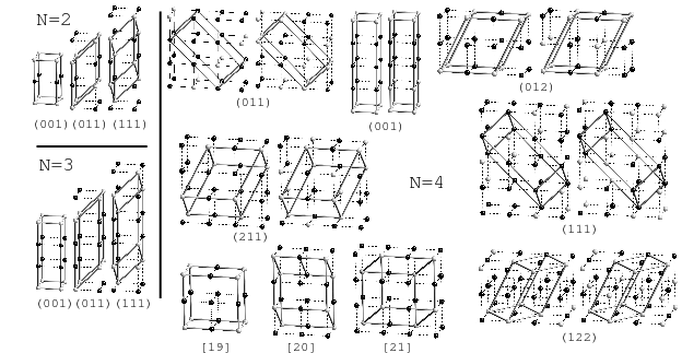
Figure 11: The first 21 binary structures derived from the simple cubic lattice. All have 4 atoms/cell or less. Structures marked with a crystallographic direction $(hkl)$ can be characterized as a stacking of pure A and B atomic layers (black and white spheres. For $n=4$ all of the stacked structures occur in pairs, A₃B₁ and A₂B₂. The last three structures, labeled 19, 20, and 21, cannot be characterized as pure stackings. These structures have basis vectors whose corresponding quotient group is $G=\mathbf{Z}_{2}\oplus\mathbf{Z}_{2}$ (rather than $\mathbf{Z}_{4}$).

Table 7 lists the number of fcc/bcc ternary and quaternary derivative structures. A figure displaying the ternary structures for $n\leq 4$ is unnecessary—the ternary structures have the same unit cell as the binary structures, only the labelings are different. For $n=3$ the labeling $aab$ is replaced by $abc$. For $n=4$ the labelings $aaab$ and $aabb$ are replaced by $aabc$ and $abac$. And, the Agd₃ structure has both labelings, rather than one.

$n$	ternary		quaternary
	structures	cumulative	structures	cumulative
3	3	3	–	–
4	13	16	7	7
5	23	39	9	16
6	130	169	110	126
7	197	366	211	337
8	1 267	1 633	2 110	2 447
9	2 322	3 955	5 471	7 918
10	9 332	13 287	32 362	40 280

Table 7: Number of ternary and quaternary derivative structures for an fcc parent lattice. Compare to the number of binary structures of Table 5. As the number of labels $k$ is increased, the number of derivative structures increases rapidly.

IV Applications

We give here a few examples of how the list of derivative superstructures can be used. An in-depth discussion of each example is beyond the scope of this paper. The full results of each example will be reported in forthcoming publications but we summarize our findings here to demonstrate how the efficient enumeration of derivative structures can be applied to discover new physics or aid in materials design.

IV.1 fcc example

Figure 2 shows small-unit-cell binary superstructures for an fcc parent lattice enumerated with our algorithm. There are 17 unique structures in the set, two for $n=2$, three for $n=3$, and 12 for $n=4$. Most of the structures can be envisioned as stackings, along different crystallographic directions, of layers containing a single kind of atom. For instance, the $n=2$ structure labeled L1₀ can be envisaged as A and B layers alternately stacked in the [001] direction. The stacking directions are indicated by green planes in the figure.

Of these 17 small-unit-cell fcc superstructures, some are well-known structures and others have never been observed (blue shading). Some have never been observed experimentally but are predictedCurtarolo et al. (2005) to be thermodynamically stable at low temperatures (yellow shading). It is intriguing to ask why, among these small, simple structures, some are observed in Nature and others are not. Recently, a metric of ‘bonding randomness’ was proposedHart (2007a) that shows structures with low bonding randomness are more likely to be observed in Nature.

In the case of these 17 fcc-derived superstructures, those that have been observed (unshaded) are generally ‘unrandom’, those that that have never been observed or even predicted to exist (blue shading) have a highly random bonding, and those in between are those that have not yet been observed but have been predicted to exist (see Fig. 4 in Ref. Hart, 2007a). Noteworthy among these results is the case of the structure predicted to exist in Cd-Pt at a 1:3 stoichiometry (see Fig. 2). We refer to this structure as L1₃ in analogy to the Strukturbericht designations for related structures.

The first theoretical discovery of the L1₃ structure was by Müller in Ag-Pd.Müller and Zunger (2001) Later, a datamining searchCurtarolo et al. (2005) found L1₃ as a candidate ground state in two binary systems, Cd-Pt and Pd-Pt. Subsequently, we constructed cluster expansions for these two systems so that the energy of any configuration could be computed quickly. Then, by enumerating all possible configurations, we performed (practically) exhaustive searches of fcc-derived superstructures and verified that this structure is globally stable in these two systems.

Because the L1₃ structure had not been observed and was not even suspected, the computational discovery of L1₃ could have never occurred without exhaustively examining derivative superstructures as we have done here. Without the enumeration, this structure never would have been considered in the searches. Our new algorithm provides a faster, more general way to enumerate derivative superstructures. It has turned up a number of unsuspected structures with low bonding randomness, which are good candidates for new structures that are likely to be observed experimentally.

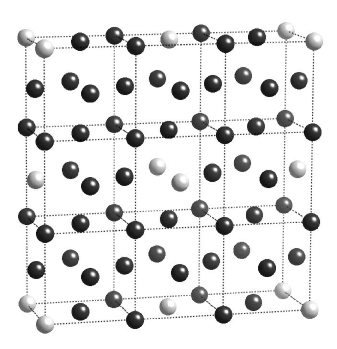
Figure 12: The fcc-derived superstructure of Pt₈Ti. The structures is shown as a face-centered tetragonal structure. The dotted lines show the conventional fcc cell. Black spheres represent Pt, white spheres Ti. This structure has the lowest bonding randomness of all 9 atom/cell fcc superstructures.

IV.2 8:1 stoichiometry example

In this example we apply the enumeration algorithm to structures with a fixed concentration. A structure with an unusual stoichiometry of 8:1 was discoveredPietrokowsky (1965) in Pt-Ti in the late 1950s (see Fig. 12). The structure was then ‘re-discovered’Quist et al. (1969); van dder Wekken et al. (1971) in Ni-Nb in 1969, and has since been observed in about a dozen more Pt/Pd/Ni-rich intermetallic systems. This structure has practical import because its impact on the alloy. Pure platinum and palladium are quite soft but the Pt₈Ti structure can significantly strengthen the material, while at the same time maintaining the purity of the host material. (International jewelery hallmarking standards require that the alloy be at least 95 wt-% pure.)

It would be useful to know which Pt/Pd-rich compounds can form stable structures and what the structures are. Using the structural enumeration method described in this paper, we generated all 9-atom/cell, 8:1 stoichiometry structures—there are 14 such structures. Taking these enumerated structures, we rankedHart (2007a) the structures and find that the Pt₈Ti structure has the highest likelihood among the 14. However, one of the other 13 structures has a likelihood index nearly as high as Pt₈Ti. Therefore it is another candidate for a new Pt/Pd/Ni-rich structures. Using first-principles methods, combined with the enumeration algorithm, we are conducting a broad search for the other high-likelihood Pt/Pd-rich structures. So far we have found 9 new binary systems that have undiscovered Pt- or Pd-rich ground states.Gilmartin et al. (2008)

IV.3 Perovskite example

Because our enumeration algorithm works for any parent lattice (i.e., it is independent of geometery), we can apply it to cases outside the realm of normal alloy questions (usually fcc- or bcc-based systems). This example demonstrates its use in ordering problems where the parent lattice is simple cubic. There is a large class of oxide compounds where the ‘configuration question’ is based on a simple cubic parent lattice.

These oxide compounds have a number of important properties such as ferroelectricity and superconductivity. Because of their important scientific and industrial applications, there is motivation to optimize their functional properties to meet different design needs. The first approach to optimizing their properties is to change the constituent elements. This approach is limited by the number of elements that will form the perovskite structure so to further tune the properties, researchers create mixtures of two (or more) different perovskites.

These oxides have the perovskites structure (see Fig. LABEL:perovskite ). The formula unit for this structure is ABO₃ where A and B are typically transition metals or late-period metals like Pb. The A atoms are octahedrally-coordinated by oxygen atoms, and the A-sites form a simple cubic lattice. The B-sites also form a simple cubic lattice in the interstitial sites of the oxygen octahedra.

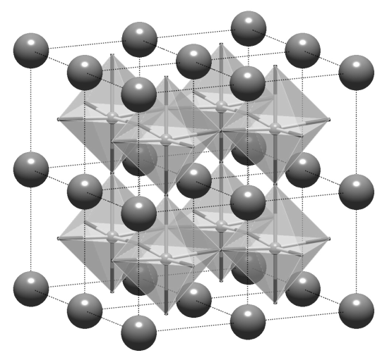
Figure 13: Depiction of the perovskite structures. B-sites are the cube corners, A-sites the cube centers. The oxygen atoms (not shown) form an octahedron around the A-sites.

In an attempt to tune the properties of perovskite materials, researchers often introduce a third metal. For B-site mixing, the formula unit then becomes AB_1-xB${}^{\prime}_{x}$O₃. The atoms on the substitution sites will often order, resulting in a superstructure larger than the original cubic unit cell. Because the ordering also affects the materials properties (sometimes drastically), it is helpful to know what ordered structures are possible and which are likely. This is precisely the information that our algorithm gives.

The B-sites of the perovskite structure form a simple cubic lattice as shown in the figure (big spheres). To find all possible orderings of B and B^′ atoms on the B site, we apply our algorithm to the case of a simple cubic superstructures. For unit cells with 4 B-atoms or less per unit cell, we find 21 possible structures (see Table 6 and Fig. 11).

A number of these superstructures have been observed.Krause et al. (1979); Chen et al. (1989); Randall et al. (1987); Fang and Zhang (1995); King et al. (1988) For $n=2$, all three types have been observed. For $n=3$, the (111) oriented structure has been observed. The only $n=4$ structure that we are aware of is the A₃B₁ structure that we have labeled [21] in Fig. 11. Apparently, only these five structures have been observed in B-site mixed perovskites. Whether or not there are other structures that are likely awaits further exploration, but our algorithm provides a starting point for finding complex perovskites with new structures.

IV.4 Ternary fcc structures

The two important generalizations of our algorithm over the FWZ method are arbitrary parent lattices and arbitrary numbers of labels (atom types). The second means we can treat cases beyond binaries, $k>2$. In the following example we exploit the latter generalization to examine ordered ternary intermetallics.

Ordered binary intermetallics offer advantages over conventional disordered alloys for structural applications at high temperatures. But they also have disadvantages. Although they typically have high moduli, melting points, and strain hardening rates, they suffer from low ductility and brittle failure. One would like to develop alloys which can retain the advantages but avoid the problem of poor ductility.

Cubic L1₂-like alloys often meet the ductility requirement but unfortunately occur in nickel, cobalt, and platinum based binary alloys which are too dense for the desired applications. Aluminum-rich alloys would therefore be attractive but for the fact that most binary aluminum compounds are not cubic. Thus we need a way to form cubic alloys with lightweight constituents.

One promising avenue is multicomponent alloys ($k>2$), primarily ternaries. Adding a third component to a binary alloy that forms L1₂-like structures such as D0₂₂ often induces a cubic phase that is more ductile. Although much work has pursued this avenue,not (e); Kumar (1990) there are significant experimental difficulties in identifying phases, determining sublattice compositions, and discerning crystal structure of ordered phases. Computational modeling is complementary to the experimental effort.

Our algorithm/code provides an important component to modeling efforts. Coupled with a ternary cluster expansionWolverton and de Fontaine (1994); Ceder et al. (1994) code we recently developed, we can now exhaustively explore the space of possible structures in ternary intermetallics. The number of ternary fcc superstructures is vastly larger than the number of binary structures (compare Table 7 and Table 5), so a systematic approach like ours is even more important. The enumerated ternary structures would also be useful in a datamining approach like that of Ref. Curtarolo et al., 2005.

V Summary

We developed an algorithm for enumerating derivative structures. The algorithm first generates all unique superlattices by enumerating all Hermite normal form matrices and using the symmetry operations of the parent lattice to eliminate rotationally equivalent superlattices. Next, the algorithm generates all possible atomic configurations (labelings) of each superlattice and eliminates duplicates using a group-theoretical approach rather than geometric analysis.

The algorithm is exceptionally efficient due to the use of (i) perfect, minimal hash tables and (ii) a group-theoretical approach to eliminating duplicate structures. These two features result in a linearly scaling algorithm that is orders of magnitude faster than the previous method. Moreover, the method can be applied to any parent lattice and to arbitrary $k$-nary systems (binary, ternary, quaternary, etc.). The method is formally complete (does not undercount) and key parts of the algorithm (and its implementation) can be rigorously checked by number theory results and Burnside’s lemma.

We presented results for the number of superlattices and derivative structures for several different parent lattices as well as binary, ternary and quaternary systems. Additionally, applications of the algorithm to alloys were demonstrated. We coupled the results with cluster expansions and the geometric approach of Ref. Hart (2007a) and (i) provided evidence of an altogether new intermetallic structure, L1₃, in Cd-Pt and Pd-Pt, (ii) found the novel Pt₈Ti to be the most likely structure for 8:1 fcc derivative structures and uncovered another possible new prototype, (iii) enumerated small-unit-cell structures of perovskite alloys, providing possible new structures for materials design, (iv) demonstrated how the method can be applied to aid ternary alloy design.

VI Acknowledgments

G. L. W. H. gratefully acknowledges financial support from the National Science Foundation through Grant No. DMR-0650406. G. L. W. H. thanks Martin L. Searcy and Bronson S. Argyle for useful discussions concerning algorithm development and implementation of hash tables and hash functions. We also wish to thank Axel van de Walle whose input was helpful in testing the code.

VII Author Contributions

G. L. W. H. conceived the project, implemented the algorithm in Fortran 90, and wrote the first draft of the paper. The algorithm was developed jointly but key components were invented by R. W. F, who also implemented the algorithm in Maple as a check on the Fortran implementation. Both authors contributed to the manuscript.

VIII Appendix

Hermite Normal Form: If $L$ is a lattice, with basis given by the columns of a square matrix $\mathbb{A}$, and $S$ is a superlattice, then $S$ will have basis $\mathbb{AM}$ where $\mathbb{M}$ is a square matrix of integers. Furthermore, all bases of $S$ will have the form $\mathbb{AMN}$ where $\mathbb{N}$ is an integer matrix with determinant $\pm 1$. Thus, to find a canonical basis for $S$, we may use elementary integer column operations on $\mathbb{M}$ to make it lower triangular, with positive entries down the diagonal. Furthermore, we can arrange that the lower triangular matrix $\mathbb{H}=\mathbb{MN}$ have the property that every off-diagonal element is less than the diagonal element in its row. Such a matrix $\mathbb{H}$ is said to be in Hermite Normal Form, and is unique with respect to the matrix $\mathbb{M}$.

Thus, if the determinant of $\mathbb{M}$ is $n$, then the number of superlattices $S$ of $L$ with index $n$ is equal to the number of distinct HNF matrices with determinant $n$. In 3 dimensions, that number is

$$\sum_{d\big{|}n}d\>\sigma(d)=\prod_{i=1}^{k}\Biggl{(}{(p_{i}^{e_{i}+2}-1)(p_{i}^{e_{i}+1}-1)\over(p_{i}-1)^{2}(p_{i}+1)}\Biggr{)},$$

where $n=\prod p_{i}^{e_{i}}$ is the prime factorization of $n$.

Smith Normal Form: Using elementary integer row and column operations (adding or subtracting an integer multiple of one row or column to another, multiplying a row or column by $\pm 1$, or exchanging two rows or columns), we may reduce the integer matrix $\mathbb{M}$ to a diagonal matrix $\mathbb{D}$ with the following properties:

(i) Each diagonal entry of $\mathbb{D}$ divides the next one down.

(ii) The product of the diagonal entries of $\mathbb{D}$ is the absolute value of the determinant of $\mathbb{M}$.

This is called the Smith Normal Form of $\mathbb{M}$. In the lattice case, where $L$ is a lattice with basis $\mathbb{A}$, and $S$ is a superlattice (subgroup) with basis $\mathbb{AM}$, then $\mathbb{D}$ describes the quotient group $L/S$ as a direct sum of cyclic groups. The diagonal entries of $\mathbb{D}$ are the orders of the cyclic direct summands of the quotient group (as in the Fundamental Theorem of Finite Abelian Groups). For example, using the notation ${\bf Z}_{n}={\bf Z}/n{\bf Z}$, if $D=\begin{pmatrix}D_{11}&0&0\cr 0&D_{22}&0\cr 0&0&D_{33}\cr\end{pmatrix}$, then

$$L/S\cong G={\bf Z}_{D_{11}}\oplus{\bf Z}_{D_{22}}\oplus{\bf Z}_{D_{33}}.$$

A simple, two dimensional example, may help to show how this affects our lattice labeling problem. Consider the three matrices (all in HNF form)

$$\mathbb{H}_{0}=\begin{pmatrix}2&0\cr 0&4\cr\end{pmatrix}\hskip 21.68121pt\mathbb{H}_{1}=\begin{pmatrix}2&0\cr 1&4\cr\end{pmatrix}\hskip 21.68121pt\mathbb{H}_{2}=\begin{pmatrix}2&0\cr 2&4\cr\end{pmatrix}.$$

The matrices $\mathbb{H}_{0}$ and $\mathbb{H}_{2}$ both reduce to the SNF matrix $\begin{pmatrix}2&0\cr 0&4\cr\end{pmatrix}$, which corresponds to a quotient group which is Abelian, but not cyclic, but the middle matrix, $\mathbb{H}_{1}$, reduces to SNF matrix $\begin{pmatrix}1&0\cr 0&8\cr\end{pmatrix}$, corresponding to the cyclic group of order 8. Thus, if we take $\mathbb{A}$ to be the identity matrix, so $L={\bf Z}^{2}$, and let $S_{i}$ be the lattice with basis $\mathbb{H}_{i}$, then $L/S_{0}$ and $L/S_{2}$ are each isomorphic to the group ${\bf Z}_{2}\oplus{\bf Z}_{4}$, while $L/S_{1}$ is isomorphic to the cyclic group of order 8.

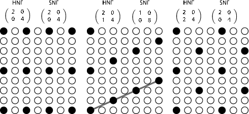
Figure 14: Two-dimensional superlattices of index $n=8$. The first and third share the same SNF while the second has the trivial SNF, implying a purely cyclic quotient group. In contrast to the first and third superlattices, the lattice points in layers parallel to the superlattice edge (dotted line) must all have the same label.

The fact that the latter is cyclic means we can layer the parent lattice in such a way that each parallel layer consists of points which all must get the same label (see Fig. 14). We can arbitrarily label each layer passing through the interior points of the basis parallelogram, and label the rest of the lattice cyclically, as if labeling a one-dimensional lattice. The quotient group for $S_{0}$ or $S_{2}$ is not cyclic but can just as easily be used to determine equivalent labelings.

In general, SNF provides a natural homomorphism from the parent lattice $L$ onto the direct-sum group $G={\bf Z}_{D_{11}}\oplus{\bf Z}_{D_{22}}\oplus{\bf Z}_{D_{33}}$, with kernel $S$. By the First Homomorphism Theorem, it effectively gives an isomorphism from $L/S$ to $G$. Since we do only elementary integer row and column operations, we may write $\mathbb{D}=\mathbb{PMQ}$, where the transition matrices $\mathbb{P}$ and $\mathbb{Q}$ are integer matrices with determinant $\pm 1$. Note that $\mathbb{AMQ}$ is another basis for $S$, so an element $x\in S$ iff $\mathbb{MQ}z=\mathbb{A}^{-1}x$ for some integer column vector $z$, which is true iff $\mathbb{D}z=\mathbb{PA}^{-1}x$. So the map

$$x\;\mapsto\;\mathbb{PA}^{-1}x\;\Biggl{(}{\rm mod}\;\begin{pmatrix}D_{11}\cr D_{22}\cr D_{33}\cr\end{pmatrix}\Biggr{)},$$

(meaning that each row of the resulting column matrix is reduced modulo the corresponding diagonal element of $\mathbb{D}$) maps from $L$ into the direct sum group $G$, with its kernel being the superlattice $S$.

As for computing the SNF of a matrix, there are special algorithms designed to compute it efficiently when $\mathbb{M}$ is very large but the simplest algorithm, effective for small (e.g., 3$\times$3) matrices, is basically an extension of Euclid’s algorithm for finding the greatest common divisor of two numbers. One subtracts multiples of elements in the matrix from other elements in the same row or column (using column or row operations respectively) until the greatest common divisor of all the elements of $\mathbb{M}$ is exposed. That element is then moved to the upper left corner of the matrix and used to zero out all other elements in the first row and in the first column. Then one applies the same algorithm to the 2 by 2 submatrix in the lower right. Thus, in particular, the upper left entry in $\mathbb{D}$ is always the greatest common divisor of all the entries in $\mathbb{M}$.

Note that the number of $3\times 3$ SNF matrices with determinant $n$ is given by $\prod_{i}P_{3}(e_{i})$, where $n=\prod_{i}p_{i}^{e_{i}}$ (the prime factorization) and $P_{3}(k)$ is the number of partitions of an integer $k$ using at most 3 summands.not (f)

References

- Buerger (1947) M. J. Buerger, Journal of Chemical Physics 15, 1 (1947).
- not (a) In the mathematical literature, and in some of the crystallography literature, these derivative lattices are referred to as sublattices. Although this nomenclature is more correct from a mathematical/group theory point of view, we follow the nomenclature typically seen in the physics literature where a lattice (or a structure) whose volume is larger than that of the parent is referred as a superlattice (or a superstructure).
- Santoro and Mighell (1973) A. Santoro and A. D. Mighell, Acta Crystallographica Section A 29, 169 (1973).
- Santoro and Mighell (1972) A. Santoro and A. D. Mighell, Acta Crystallographica Section A 28, 284 (1972).
- Kim et al. (2005) K. Kim, P. A. Graf, W. B. Jones, and G. L. W. Hart, Appl. Phys. Lett. 87, 243111 (2005).
- Ferreira et al. (1991) L. G. Ferreira, S.-H. Wei, and A. Zunger, The International Journal of Supercomputer Applications 5, 34 (1991).
- van de Walle and Ceder (2002) A. van de Walle and G. Ceder, Journal of Phase Equilibria 23, 348 (2002).
- van de Walle et al. (2002) A. van de Walle, M. Asta, and G. Ceder, CALPHAD 26, 539 (2002).
- Zarkevich et al. (2007) N. A. Zarkevich, T. L. Tan, and D. D. Johnson, Physical Review B (Condensed Matter and Materials Physics) 75, 104203 (pages 12) (2007).
- not (b) We believe that these restrictions in the FWZ algorithm have been overcome in the other implementations cited above, though there are no publications that discuss these modern implementations explicitly. However, our algorithm is conceptually different and completely general—geometrical considerations are not central to the enumeration as in the FWZ approach. Moreover, our approach is far more efficient and scales linearly—the running time of the algorithm is directly propotional to the the number of unique structures found.
- Curtarolo et al. (2005) S. Curtarolo, D. Morgan, and G. Ceder, Calphad 29, 163 (2005).
- Sloane (a) N. J. A. Sloane, The on-line encyclopedia of integer sequences.
- Billiet and Le Coz (1980) Y. Billiet and M. R. Le Coz, Acta Crystallographica Section A 36, 242 (1980).
- Rutherford (1992) J. S. Rutherford, Acta Crystallographica Section A 48, 500 (1992).
- Liskovets and Mednykh (2000) V. A. Liskovets and A. Mednykh, Commun. in Algebra 28, 1717 (2000).
- Baake (1997) M. Baake, Mathematics of Long-Range Aperiodic Order (Kluwer Academic, 1997), chap. Solution of coincidence problem in dimensions , pp. 9–44.
- Stanley (1999) R. P. Stanley, Enumerative Combinatorics,, vol. 2 (Cambridge University Press, 1999).
- Sloane (b) N. J. A. Sloane, Sublattices of index n in generic 3-dimensional lattice.
- Hart (2007a) G. L. W. Hart, Nature Materials 6, 941 (2007a).
- Hart (2007b) G. L. W. Hart, Phys. Rev. B (to be submitted). (2007b).
- not (c) In the implementations of Refs. van de Walle and Ceder, 2002; van de Walle et al., 2002; Zarkevich et al., 2007, the structures appear to be compared directly in a geometric sense, requiring an search. In the FWZ algorithm, a subset of the correlations between sites in each structure are computed and then these correlations are compared, still an search. Because the subset of correlations is limited by its nature, this approach is formally incomplete.
- not (d) An analytical check on the counting for these kinds of duplicates can be found in Rutherford’s work.Rutherford (1995).
- (23) In three dimensions, each member of the quotient group formally has three components, even though in many cases only one is non-trivial. For example, if the diagonal elements of the SNF of a superlattice are (1, 1, 4), then the 4 members of the image group are (0,0,0), (0,0,1), (0,0,2), and (0,0,3). On the other hand, if the diagonal elements of the SNF are (1,2,2), then the 4 members of the image group are (0,0,0), (0,0,1), (0,1,0), and (0,1,1).
- (24) J.-O. Moussafir, Three-dimensional simplices of determinant n.
- Müller and Zunger (2001) S. Müller and A. Zunger, Phys. Rev. Lett. 87, 165502 (2001).
- Pietrokowsky (1965) P. Pietrokowsky, Nature 206, 291 (1965).
- Quist et al. (1969) W. E. Quist, J. van der Wekken, R. Taggart, and D. H. Polonis, Trans. Met. Soc. AIME 245, 345 (1969).
- van dder Wekken et al. (1971) J. van dder Wekken, R. Taggart, and D. H. Polonis, Metal Science Journal 5, 219 (1971).
- Gilmartin et al. (2008) E. Gilmartin, J. Corbitt, and G. L. W. Hart, in March APS Meeting Bulletin 2008 (American Physical Society, 2008).
- Krause et al. (1979) H. Krause, J. Cowley, and J. Wheatley, Acta Crystallographica Section A 3, 1015 (1979).
- Chen et al. (1989) J. Chen, H. Chan, and M. Harmer, J. Am. Ceram. Soc. 72, 829 (1989).
- Randall et al. (1987) C. Randall, D. Barber, R. Whatmore, and P. Groves, Ferroelectrics 76, 277 (1987).
- Fang and Zhang (1995) F. Fang and X. Zhang, J. Mater. Res. 10, 1582 (1995).
- King et al. (1988) G. King, E. K. Goo, T. Yamamoto, and K. Okazaki, J. Am. Ceram. Soc. 71, 454 (1988).
- Kumar (1990) K. S. Kumar, International Materials Reviews 35, 293 (1990).
- not (e) The literature for ternary substitutions in L12-like binary compounds is vast. For a representative survey, see the review by Kumar.Kumar (1990).
- Wolverton and de Fontaine (1994) C. Wolverton and D. de Fontaine, Phys. Rev. B 49, 8627 (1994).
- Ceder et al. (1994) G. Ceder, G. D. Garbulsky, D. Avis, and D. de Fontaine, prb 49, 1 (1994).
- not (f) The partition idea was introduced into the crystallographic literature in Ref. Kucab, 1981.
- Rutherford (1995) J. S. Rutherford, Acta Crystallographica Section A 51, 672 (1995).
- Kucab (1981) M. Kucab, Acta Crystallographica Section A 37, 17 (1981).