Initial Conditions For Large Cosmological Simulations

Abstract

This technical paper describes a software package that was designed to produce initial conditions for large cosmological simulations in the context of the Horizon collaboration. These tools generalize E. Bertschinger’s Grafic1 software to distributed parallel architectures and offer a flexible alternative to the Grafic2 software for “zoom” initial conditions, at the price of large cumulated cpu and memory usage. The codes have been validated up to resolutions of $4096^{3}$ and were used to generate the initial conditions of large hydrodynamical and dark matter simulations. They also provide means to generate constrained realisations for the purpose of generating initial conditions compatible with, e.g. the local group, or the SDSS catalog.

1. Introduction

Numerical simulations have proved to be valuable tools in the field of cosmology and galaxy formation. They provide a mean to test theoretical assumptions, to predict the properties of large scale structures (and galaxies within) and give access to synthetic observations without sacrifying the whole complexity that arise from non-linearities. Thanks to the recent progresses in terms of numerical techniques and available hardware, numerical cosmology has become one of the most important (and CPU consumming) field among the scientific topics that require extreme computing. Over the last few years, a series of large simulations have been produced by, among others, Cen and Ostriker (2000), the Virgo Consortium (Frenk et al. 2000, the Millenium: Springel et al. 2005), Weinberg et al. (2002), the Gasoline team (Wadsley et al. 2004). Following the same route, the purpose of the Horizon Project is to federate numerical simulations activities within the french comunity on topics such as : the large scale structure formation in a cosmological framework, the formation of galaxies and the prediction of its observational signatures. The collaboration studies the influence on the predictions of the resolution, the numerical codes, the self-consistent treatment of the baryons and of the physics included.

These investigations are performed on initial conditions (ICs thereafter) that share the same phases and their production is described in the current paper. The large Horizon ICs involves two boxes of 50 and 2000 Mpc/h comoving size with respectively $1024^{3}$ and $4096^{3}$ initial resolution elements (particles or grid points), following a $\Lambda$CDM concordance cosmogony. They were generated from an existing set of initial conditions created for the ’Mare Nostrum’ simulation (Gottlöber and Yepes 2007): they share the same phases but with different box sizes and resolutions. The ($50h^{-1}$Mpc,$1024^{3}$) ICs were used as inputs to the AMR code RAMSES (Teyssier 2002) in a simulation that included dark matter dynamics, hydrodynamics, star formation, metal enrichment of the gas and feedback. This simulation directly compares to the Mare-Nostrum simulation in terms of cosmology and physics and it will be refered as the Horizon-MareNostrum simulation hereafter(Ocvirk, Pichon and Teyssier 2008). The ($2000h^{-1}$Mpc,$4096^{3}$) ICs served as a starting point for the Horizon-4$\Pi$ simulation(Teyssier et al. 2007, http://www.projet-horizon.fr): it is a pure dark matter simulation and assumes a cosmology constrained by WMAP3. It is currently used to investigate the full-sky gravitational lensing signal that could be observed by the DUNE experiment (hence the $4\Pi$).

The paper is organised as follows: first, we briefly explain the principle of the ICs’ generation. Then we describe how the phases were extracted from the MareNostrum ICs in order to make the Horizon ICs consistent with this reference. We describe next the features of a series of codes used to generate and process the different Horizon ICs:

• mpgrafic: ICs generation with optional low-frequency constraints

• constrfield: Low-frequency ICs generation with point-like constraints.

• degraf: Low-pass filtering and resampling of ICs

• powergrid: ICs empirical power spectrum estimation.

• splitgrafic: Estimation of matter density on a grid from a set of particle positions, and Peano-Hilbert domain decomposition.

Finally we illustrate how these codes were implemented on the two Horizon simulations.

2. Random Field for Cosmological Initial Conditions

2.1. Grid-based initial conditions

For completeness, we quickly review the principle of ICs generation. Most of the following has been strongly inspired from articles by Pen (1997) and Bertschinger (2001). Let us consider the initial 3D gaussian random field $\delta({\bf x})$, representing the density or the displacements, and let us define its Fourier transform $\delta({\bf k})$. If we consider zero-mean fields, they are completely defined by their correlation function or, equivalently, by their power spectra, $P(k)$:

$$P(k)\delta_{D}({\bf k}-{\bf k^{\prime}})=\langle\delta({\bf k)\delta^{*}({\bf k^{\prime})\rangle.}}$$ (1)

All the statistical information in a gaussian homogeneous and isotropic realization is contained in this quantity and the difficulty of generating initial conditions resides in obtaining a field which has the correct power spectrum.
We chose to follow the convolution-based method described by e.g Pen (1997) and define the correlation kernel in Fourier space as:

$$A(k)=\sqrt{P(k)}.$$ (2)

To reproduce the correlation function accurately one may need to first convolve the power spectrum with the window that describes the simulation box, as advocated by Pen (1997). The influence of the box size on rms density in spheres of given radius (which are relevant for mass function estimates of collapsed objects), is negligible for sphere radii much smaller than the box length, even for simulations designed to study galaxy cluster scales.

Then the ICs generation is a two-step procedure. First a normal, uncorrelated random field of unit variance is generated in position space. This white noise $n_{1}({\bf x})$ has a constant power spectrum, e.g.:

$$\langle|n_{1}({\bf k)}|^{2}\rangle=1.$$ (3)

The second step involves convolving the white noise with the correlation kernel in order to obtain the initial fluctuation field:

$$\delta({\bf x})=n_{1}({\bf x})*A({\bf x}),$$ (4)

or in Fourier space

$$\delta({\bf k})=n_{1}({\bf k})A({\bf k}).$$ (5)

It can be easily seen that $\langle|\delta({\bf k})^{2}|\rangle{}=P(k)$ and the initial field automatically has the correct power spectrum.

One of the main virtue of the method resides in the possibility of using the same white noise for different power spectra. In other words, it decouples explicitely the phases (which contain the specificities of a given realization in terms of relative positions) from the amplitudes of the fluctuations (corresponding to one’s favorite choice of cosmological model). A change in the physics or in the box size results in a change of the convolution kernel, but the underlying structure of the field will remain globally the same for a given white noise realization. Conversely, Eq. 5 implies that the initial phases can be recovered from a set of ICs, provided that the convolution operation can be inverted. In other words, it is possible to generate a new set of ICs from an old one (see Section 4) and such a set would share the same overall structures with e.g. a modified cosmology or box size.

2.2. Grid-based versus particle-based initial conditions

In numerical simulations, the dark matter distribution is almost exclusively described in terms of particles and this discretized description is also applied to the gas in SPH-like hydrodynamical codes. Consequently, dealing with ’particle-type’ data is the most frequent case while the current procedure naturally deals with densities and velocities sampled on a grid. This can be easily tackled by recalling the density-velocity relation that is valid in the linear regime :

$$\frac{1}{aH}\nabla_{{\bf x}}{\bf u}=-f(\Omega_{m},\Omega_{\Lambda})\delta({\bf x}).$$ (6)

Here ${\bf u}$ stands for the comoving peculiar velocity, ${\bf x}$ for the comoving position, $H$ for the Hubble constant, $a$ for the scale factor and $f$ is defined as the logarithmic time derivative of the growth factor:

$$f(\Omega_{m},\Omega_{\Lambda})\equiv\frac{{\mathrm{d}}\log D^{+}}{{\mathrm{d}}\log a}.$$ (7)

Functional fits for $f$ can be found in the literature (e.g. Lahav et al. 1991) or be directly computed for a given cosmology. Hence, assuming that particles were displaced from a regular grid and knowing their velocities, the initial density field can be directly recovered from Eq. (6). One can see that the (eulerian) positions of particles are not directly involved in this procedure; however, their lagrangian coordinates are used to remap the particle velocities to grid cells.

3. Grid-based ICs: Technical Implementation

Once the “phases” (the white noise) are chosen on a grid of a given size, it is possible to use them to generate initial density and velocity realizations with the desired cosmology and power spectrum, at resolutions that can differ from the initial white noise realization.

According to linear theory, which applies for initial conditions , density and velocity divergence are related through Eq. (6), so that a single white noise realization determines both density and velocities on a grid of equal size (see e.g. Bertschinger 2001).
A first numerical implementation of this algorithm was made by E. Bertschinger in the package Grafic1. We extend here his code using the Message Passing Interface (MPI) library to deal with large simulation cubes on distributed memory platforms. Another implementation of MPI-based Initial Conditions generator in the context of the GRACOS code is described in Shirokov (2007), http://www.gracos.org.
We also develop a few tools (low-pass filtering and resampling, power spectrum estimation, estimation of matter density on a grid from a set of particle positions) that work as well in parallel environments. We describe these tools and their usage in the following subsections.

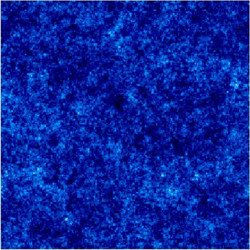
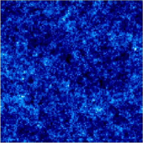
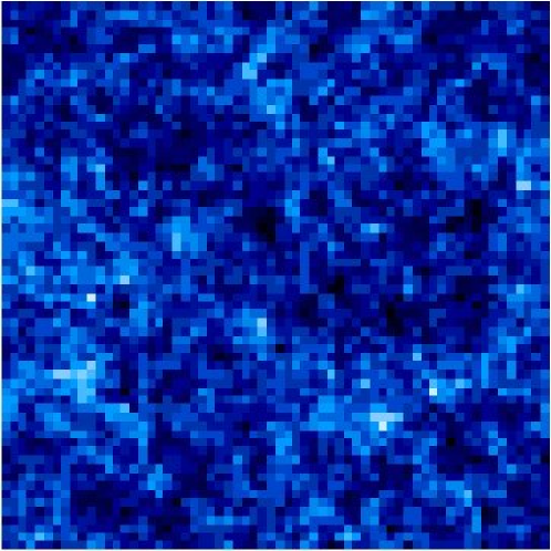
Figure 1.— The left image shows a slice of a density field realization of size $256^{3}$. The middle and right images show respectively slices of the cubes of size $128^{3}$and $64^{3}$obtained from the first density field by lowpass filtering and subsampling. The images have been rescaled to the same size to ease their comparison. The initial density field was obtained using mpgrafic with the parameters of Table 2. The low-frequency, resampled fields were obtained with the degraf utility.

3.1. Mpgrafic: a parallel version of Grafic1

Generating initial conditions for cosmological simulations on a grid from an initial white noise realization is theoretically quite simple, as it involves a straightforward implementation of Equations (5) and (6) in Fourier space. Indeed, the main issues in the Grafic1 code involve getting the normalization right (in terms of $\sigma_{8}$ or $Q_{{\rm rms}}$, which are input parameters), and therefore in the cosmology routines.

3.1.1 Description

Difficulties of a more technical nature appear as the size of the desired cubes (and/or the number of particles) grow and that a single cube does not fit into a computer’s memory. An elegant answer to this problem, in the context of multi-resolution (“zoom”) initial conditions was designed by Bertschinger (2001) and implemented in the Grafic2 package. This solution involves generating a low resolution cube first, and successively adding higher frequencies in nested sub-regions, constrained by the phases of the already existing low frequency modes. Strictly speaking, the exact solution to this problem is (naively) as costly as the direct generation of the full cube at the highest resolution, but approximate, less costly solutions based on anti-aliasing kernels can be designed. This is precisely what is done in the Grafic2 package.

The main advantage of this solution is to produce multi-resolution initial conditions with a very reasonable memory usage, but it also has drawbacks, namely its complexity, and its built-in restrictions on the nested cubes structure of a given maximum size. Given the growing size of computer clusters, our “brute force” approach to the problem based on parallelism becomes possible, and it is also in some ways more flexible. First of all, it allows for a direct generation of global initial conditions for very large cosmological simulations. Secondly, it also allows, together with associated tools for low-pass filtering and resampling, to create multi-resolution simulations of a more general structure by simply extracting the desired sub-regions from the series of “downgraded” cubes (obtained by low-pass filtering and resampling of the initial large high-resolution cube).

There are two issues that arise when implementating a parallel (MPI-based) version of the Grafic1 software. The first involves performing efficient three-dimensional fast fourier transforms (FFTs thereafter); this difficulty is solved by using the parallel version of the FFTW library, which uses a slab domain decomposition. The second difficulty lies in the input/output. Indeed, we decided to keep the binary (Fortran) structure of the files in the Grafic1 format. In a parallel environment where each MPI process is responsible for one chunk of data, this lead us to write part of the I/O subroutines in C using reentrant read/write routines, wrapped in fortran90 to be callable from the main program.

Finally, apart from the parallelism of mpgrafic, we have added a few new features to the original Grafic1 code. An implementation of the matter power spectrum with baryon oscillations was introduced, as described in Eisenstein and Hu (1998). Secondly, the possibility of constraining the low frequency phases of the density and velocity realizations was implemented, with the input of a given white noise cube of lower resolution. This allowed us to use the same set of initial condition phases for cosmological simulations at different resolutions. Lastly, we have implemented the possibility of constraining the value of the density or velocity field values, as well as their gradients and hessians at a chosen set of positions. We will come back in more details on this last point in a following section, as it is a non-trivial extension of the code.

3.1.2 Code installation and parameter file structure

A prerequisite to use mpgrafic is to have (of course) a valid MPI library installed, including a fortran90 compiler. A second prerequisite is to have the fftw-2.1.5 library installed, with the --enable-mpi --enable-type-prefix options at the configure step. The first option builds the static and shared FFTW MPI-based libraries, the second is for the type (float or double) naming scheme of the libraries.

Note that the default build of FFTW corresponds to double precision, whereas the default type in mpgrafic is single precision. To change to single precision realizations, you need to make the single precision FFTW MPI libraries by adding the --enable-float at configure time. To compile mpgrafic in double precision mode, you need to configure with the --enable-double keyword.

The code usage has been kept as close as possible to the Grafic1 code interface, except of course for the few additional options to the code. In table 2 we show an example of parameter file of mpgrafic.

Compared to the original Grafic1 parameter files, the only differences lie in the possibility of an input power spectrum with baryonic oscillations (Eisenstein and Hu 1998), and in the optional input of a small noise file to constrain the large scale phases. Otherwise, the code is called in the following way:
mpirun -np $<\#$proc$>$ mpgrafic $<$ parameter_file
Like Grafic1, it produces seven data cubes (one density file, three dark matter velocity files, and three baryon velocity files). In the file grafic1.inc, the offsets of the velocity fields is controlled by the parameters offvelb, offvelc. The redshift of the realizations is controlled by the variance of the density field on the grid, as specified by sigstart. Finally, the size of the cubes is controlled by the parameters np1,np2,np3, that can take different values and are set in grafic1.inc. Note that when these parameters are changed the code needs recompilation.

3.1.3 Illustration on a small example, power spectrum estimate

In figure 1 we show a slice of a density file realization with the parameter file displayed in Table 2, but without large scale constraints, and for np1=np2=np3=$256$. In the same figure, we show the density files of linear grid size $128$ and $64$ obtained from this realization, by low-pass filtering and subsampling. This operation has been done using the utility called degraf, that makes use of the FFTW parallel Fourier transform routines. Written in fortran90, it takes as input a collection of files in Grafic1 format, as well as some parameters in a namelist file. These parameters include the list of the input file names, the target resolution of the output files, as well as an optional shift vector allowing a global translation of the output files (with periodic initial conditions).

Finally, another utility, powergrid, uses the FFTW parallel Fourier transform routines to compute the periodogram estimate of a density field power spectrum. It allows correction for nearest grid point (NGP) or cloud in cell (CIC, linear) interpolation of a particles set to the computation grid. Note that this resampling of a discrete density field given by particles onto grid cells leads not only to a smoothing of the grid Fourier modes (this can be corrected by the code) but also to some power aliasing, that cannot be corrected, unless prior knowledge of the density power spectrum is available. These points will be illustrated in the next section, for the Horizon simulations. Of course, none of these problems appear if one is only interested in computing the periodogram of the IC grid-sampled density fields. Figure 2 shows the theoretical power spectrum corresponding to the density field realization shown in Figure 1, together with its periodogram estimate, as well as the periodograms of its low-passed, resampled versions.

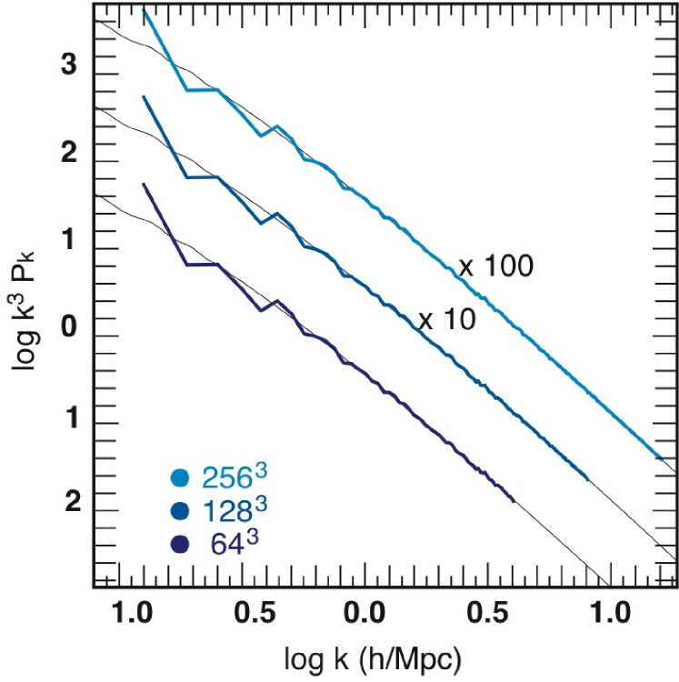
Figure 2.— Theoretical power spectrum (solid line, as output in the file power.dat by mpgrafic), together with the periodogram estimates (computed by powergrid), of the $256^{3}$density realization (top thick line), and its downgraded versions produced by degraf (middle and bottom lines for $128^{3}$and $64^{3}$ respectively).

3.2. Constrained initial conditions

Since mpgrafic opens the opportunity of generating ICs which are consistent with a given low frequency cube, it is interesting to build such a cube of phases so that the overall cube satisfy (low frequency) point like constraints on a given set of points. These constraints fix the mean value of the density or velocity field, as well as their gradients and hessians, computed at a chosen set of positions, for a given smoothing length $R_{p}$ (see Equation 11 below). Once such a low-frequency cube has been generated, it is then whitened, and set as an input to mpgrafic, which is then used to add small scale power and to resample the field according to the new Nyquist frequency .

This procedures allows for instance to generate initial conditions which are consistant with, say a given merging event, or the structure of the Local Group, the large scale structures derived from large surveys such as the SDSS (Adelman-McCarthy and for the SDSS Collaboration 2007), the 2dF (Percival et al. 2001), 2Mass (Jarrett et al. 2003), the Local Group (Mohayaee and Tully 2005), etc.

The ensemble of unconstrained gaussian random fields is defined by all possible realizations of the field values $\delta({\bf x})$, or their Fourier amplitudes $\delta({\bf k})$, for a given power spectrum. If we impose the constraints on the field, the statistical ensemble narrows down to a subset of realizations, those that have the constraints satisfied. In particular, for a discrete representation of the field on a grid of size $N^{3}$, this means that not all $N^{3}$ values of $\delta({\bf x})$ are real degrees of freedom. Averaging over the constrained ensemble $\langle\ldots\rangle_{c}$ makes both the mean $\langle\delta({\bf x})\rangle_{c}$ and the variance dependent on position ${\bf x}$.

We shall be dealing with linear constraints each of which, in general, sets a linear functional relation $V_{a}[\delta({\bf x})]$ (we will use latin letters to index the constraints where each constraint is defined by a grid position ${\bf x}_{a}$ and a constraint operator $Y_{a}$, see below) between field values to a given value, $V_{a}[\delta({\bf x})]=\tilde{V}_{a}$.

Fourier space	Configuration space	Physical meaning
$Y({\bf k})=1$	$V[\delta]=\delta$	density value
$Y({\bf k})=-\imath{\bf k}_{i}/k^{2}$	$V[\delta]=-\nabla_{i}\Delta^{-1}\delta$	linear displacement
$Y({\bf k})={\bf k}_{i}{\bf k}_{j}/k^{2}-\frac{1}{3}\delta_{ij}$	$V[\delta]=(\nabla_{i}\nabla_{j}\Delta^{-1}-\frac{1}{3}\delta_{ij})\delta$	flow shear
$Y({\bf k})=\imath{\bf k}_{i}$	$V[\delta]=\nabla_{i}\delta$	density gradient
$Y({\bf k})=-{\bf k}_{i}{\bf k}_{j}$	$V[\delta]=\nabla_{i}\nabla_{j}\delta$	density curvature

Table 1Different type of point -like constraints

Alternatively, we can take a point of view that such a restricted ensemble defines a new (constrained) random field $\delta_{c}({\bf x})$ which is still gaussian (due to the linearity of imposed relations) but is statistically inhomogeneous. Under these conditions, the well known way to construct a constrained field from unconstrained realizations is

$$\delta_{c}({\bf x})=\delta({\bf x})+\sum_{ab}\langle\delta({\bf x})V_{a}[\delta]\rangle\langle V_{a}[\delta]V_{b}[\delta]\rangle^{-1}\left(\tilde{V}_{b}-V_{b}[\delta]\right)\,.$$ (8)

(see e.g. Bardeen et al. 1986; Hoffman and Ribak 1991). In this expression, the random quantities on the right-hand side are unconstrained $\delta(x)$. Here $\tilde{V}_{b}$ is a numerical value of the constraint $b$, while $\langle\delta({\bf x})V_{a}[\delta]\rangle$ is the covariance between the field and a constraint, and $C_{ab}=\langle V_{a}[\delta]V_{b}[\delta]\rangle$ is the convariance matrix between the constraint functionals.

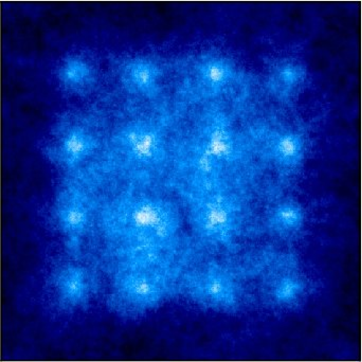
Figure 3.— Example of contrained realization generated using constrfield and extended at a $1024^{3}$resolution using mpgrafic. Here a regular grid of $4\times 4\times 4$ density peaks is imposed within a $\Lambda$CDM cosmological simulation in a box of length $100h^{-1}$Mpc. Here the constraints are of the density type, so that $Y({\bf k})=1$ for each constraint; in such a case, $V_{a}(\delta)=\delta({\bf x}_{a}$), where $delta({x}_{a})$ is the chosen constraint at position $x_{a}$.

This recipe reproduces the mean (note, the averaging is taken over all unconstrained realizations)

$$\langle\delta_{c}({\bf x})\rangle=\langle\delta({\bf x})V_{a}\rangle\langle V_{a}V_{b}\rangle^{-1}\tilde{V}_{b}\,,$$ (9)

and the correlation function

$$\langle\delta_{c}({\bf x})\delta_{c}({\bf x^{\prime}})\rangle = \xi({\bf x,x^{\prime}})-\langle\delta({\bf x})V_{a}\rangle\langle V_{a}V_{b}\rangle^{-1}\langle\delta({\bf x^{\prime}})V_{b}\rangle$$ (10)

$$+\langle\delta_{c}({\bf x})\rangle\langle\delta_{c}({\bf x^{\prime}})\rangle\,,$$

which define all statistical properties for the gaussian case.

In cosmology the primary interest is to define constraints that describe the physical properties of a patch (see e.g. Bond and Myers 1996; van de Weygaert 1996) of the density field - density, density derivatives, shear flow, averaged over the volume of the patch. Such constraints can be represented in Fourier space as

$$V_{a}[\delta]=\int d^{3}k\delta({\bf k})Y_{a}({\bf k})W(kR_{p})e^{-{\bf ikx}_{a}}\,,$$ (11)

where ${\bf x}_{a}$ is the position of the patch, $W(kR_{p})$ is a averaging filter over the patch size $R_{p}$, and $Y_{a}({\bf k})$ is the Fourier representation of the operator that specifies the constraint functional. In particular, we use the constraint types given in Table 1. Using constrained field formalism Bond et al. (1996) have demonstrated that the observed filamentary Cosmic Web of matter distribution in the Universe can be understood as dynamical enhancement of the geometrical properties of intial density field. The web is largely defined by the position and primordial tidal fields of rare events in the medium, such as precursors of large galaxies at high redshifts or clusters of galaxies at present time, with the strongest filaments between nearby clusters whose tidal tensors are nearly aligned.

The code constrfield implements the same cosmology as mpgrafic (including baryon wiggles) and offers the possibility of whitening the resulting field in order to feed it to mpgrafic as a low frequency input. An example of this procedure is illustrated in Fig. 3.

3.3. Splitting the ICs

Starting a parallel computation requires the initial conditions to be dispatched over all the computing processes. Two alternatives exist to perform this operation. The first one involves having the initial conditions to be read by a ‘master’ process and the data to be broadcasted to all the other processes, and then keep or reject the broadcasted data according to the topology of the computation’s domain split. While simple to implement, this option happens to be difficult to use in practice since broadcasting over a large number of processes can be technically problematic and time consuming.

We present an alternative option which involves having the processes upload their own set of data only. Because it is wasteful for each process to parse the whole set of initial conditions to get the relevant subset of data, this option implies that initial conditions are pre-split according to the domain decomposition strategy of the integrator. This splitting is both a domain boundary assignment, a procedure for distributing particles among the processes, and a per process file dump.

It results in a faster procedure, since each process reads its own set of data, instead of having one process reading the full initial conditions. A possible drawback lies in the fact that a splitting is defined a priori; changing the number of processes dedicated to the computation therefore requires the production of a whole new set of split initial conditions. However splitting can be performed on a single process, prior to any parallel computation, and exhibits a negligible cost in terms of CPU-time. Such a procedure can thus be applied an arbitrary number of times at almost no expense.

Horizon simulations were started from split initial conditions, where each process uploaded its own set of data. The splitting scheme followed the domain decomposition’s strategy of the cosmological calculations performed with RAMSES. It relies on a 3D Peano-Hilbert space filling curve (Salmon and Warren 1997; MacNeice et al. 2000) which provides a complete mapping between the 3D position of a grid point and a 1D coordinate on this curve. A two-dimensionnal example of such a curve is shown in figure 4. By using this piecewise linear representation of the computation domain, each process is being given a continuous portion of this curve and load balancing is achieved by ‘sliding’ the limits of the local data sets along the space-filling curve. In particular, the initial conditions are by construction well-balanced, therefore the splitting among all the processes involves a set of even subdivisions of the Peano-Hilbert curve. A $(i,j,k)$ grid point maps to a single key $q$. A set of successive $(q_{1},q_{2},...,q_{n})$ corresponds to a single process $p$.

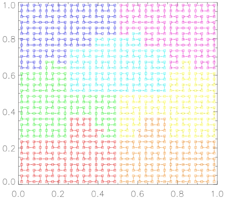
Figure 4.— Example of a ICs splitting following a Peano-Hilbert domain decomposition in two dimensions.

Note that all sub-domains are simply connected, i.e. within there are no isolated sub-regions owned by a process in the middle of another region owned by another process. For instance, in 3D, if the curve is split in $2^{r}$ sections, each section fits in a 3D rectangle of different sizes and orientations (see figure 5). Moreover, if the curve is split in $8^{r}$ parts, all the sections fit in a cube of the same volume. This type of domain decomposition is known to be most efficient if we consider the ensemble of all the refined grids configurations. It may be surpassed by other strategies (e.g. layer splitting, angular splitting) on specific situations, but Peano-Hilbert domain decomposition remains the best strategy on average.

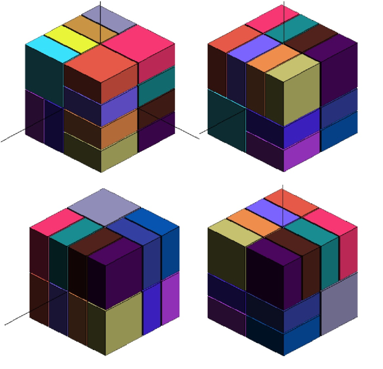
Figure 5.— Example of a ICs splitting in 16 subvolumes following a Peano-Hilbert domain decomposition as seen from four different directions.

Here we implemented a fast and simple algorithm which performs the splitting of initial conditions according to the Peano-Hilbert domain decomposition. It relies on a plane-by-plane investigation of the data cube which limits the memory consumption. Let $n^{3}$ be the number of cells in the initial conditions data cube, $F(i,j,k)$ the value of the 3D field at grid indices $1\leq i,j,k\leq n$ and $f$ a 2D slice of $F$ at index $k$. We assume that the number of processes nproc is a power of two (even though this constraint can be lifted as explained below); it ensures that each process domain is a 3D rectangle. Consequently the extent of the sub-domain corresponding to a process $p$ is given by two triplets $(i_{m},j_{m},k_{m})^{p}$ and $(i_{M},j_{M},k_{M})^{p}$ which correspond to the two extreme corners of the rectangle. The algorithm described below runs on one process only, and involves two distinct steps:

• do $k=1,n$ : loop over data planes

  • read $f=F(1:n,1:n,k)$ : the 2D data is uploaded.

  • initialisations:

    • process$(1:\mathrm{nproc})$ =.false.,

    • $(i_{m},j_{m},k_{m})^{p}=-1$, $(i_{M},j_{M},k_{M})^{p}=-1$,  $\forall p\in[1:\mathrm{nproc}]$

  • do $j=1,n$ , $i=1,n$

    • Peano-Curve mapping : (i,j,k) $\rightarrow$ q $\rightarrow$ p

    • process p is found in the k plane: process(p)=.true.

    • if process p found for the 1st time set the minimum position : if $(i_{m},j_{m},k_{m})^{p}=-1$ then $(i_{m},j_{m},k_{m})^{p}=(i,j,k)$

    • update the maximum position: if $(i,j,k)>(i_{M},j_{M},k_{M})^{p}$ then $(i_{M},j_{M},k_{M})^{p}=(i,j,k)$

  • do $p=1,\textrm{nproc}$

    • if process(p)=.false. skip : only processes detected in the plane are taken in account.

    • write f($i_{m}^{p}:i_{M}^{p},j_{m}^{p}:j_{M}^{p}$) in the file of the process p.

First, initial conditions fields are parsed plane by plane and for each plane, the process map is achieved through the space-filling curve mapping. Then for each process found in the current plane the subset of data is written in the relevant files. Because of the compacity of the sub-domains, a significant speedup can be obtained by parsing the i and j indexes of the second loop with steps larger than 1 : this procedure is safe as long as the step remains smaller than the smallest extent of the sub-domains along one direction. We call this step the speedup step. Finally the nproc$=2^{r}$ constraint can be lifted if a set of processes upload the same set of data. Each process would load a small initial condition file and would retain only its ‘sub-sub-domain’ within a sub-domain. For instance the Horizon 4$\Pi$ simulation ran on $6144=3\times 2048$ processes: the splitting was performed over 2048 sub-domains and each sub-file was uploaded by three processes. Overall, this algorithm can be quite effective and as an illustration, the $4096^{3}$ initial conditions fields of this simulation were split in 15 minutes on a single process of the CCRT computing center using a speedup step of $256$. The code ran on Itanium2 processors (double-core, but only a single core has been used here) with a $1.6$ GHz frequency.

4. Application to large Horizon simulations

Let us now illustrate on a couple of large scale simulation how mpgrafic was used. We will consider in turn a hydrodynamical and a dark matter only simulation.

4.1. Horizon-MareNostrum

The first major application of the mpgrafic code was the generation of ICs for a simulation of a cosmological hydrodynamical simulation of linear size $50h^{-1}$Mpc on a grid of size $1024^{3}$.

For the Mare Nostrum simulation, we started for technical reasons with external ICs (given as a set of particle velocities), as one of the goals was to compare two n-body plus hydro codes (namely the RAMSES and GADGET2 codes) on similar ICS. The particle velocities were therefore read from external ICs and we performed the derivation of the density field samples on the grid from the particle velocities in Fourier space, using the JMFFT Fourier Transform package. The $f$ factor involved in Eq. (7) was computed using routines provided in the original Grafic1 package. Once the velocity divergence and $f$are known, the initial density field is easily recovered and ready to be used as an input for simulations (especially for the hydrodynamical part of RAMSES), or as a source for a specific set of initial phases.

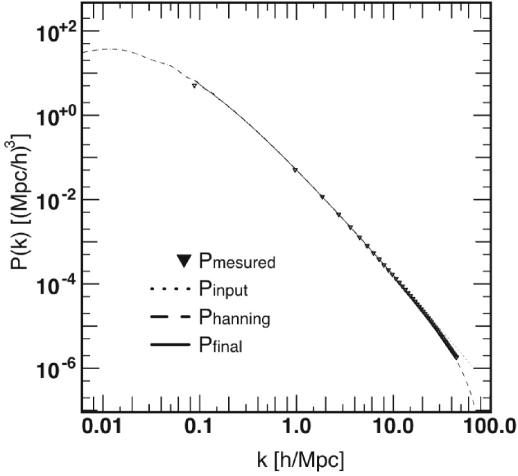
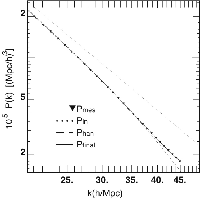
Figure 6.— The power spectrum $P(k)$ of the ’Mare Nostrum’ initial conditions. Symbols stand for the measured power spectrum, $P_{\mathrm{mes}}(k)$, while the dotted line stands for the theoretical power spectrum $P_{\mathrm{in}}(k)$. The dashed line, $P_{\mathrm{Han}}(k)$ , stand for the theoretical power spectra plus a Hanning filter contribution. The solid line, $P_{\mathrm{final}}(k)$ stand for our best fit of the power spectrum. The bottom panel represents a zoomed version of the top one where only the small scales are shown.

4.1.1 Power Spectrum Extraction from Mare Nostrum Initial Conditions

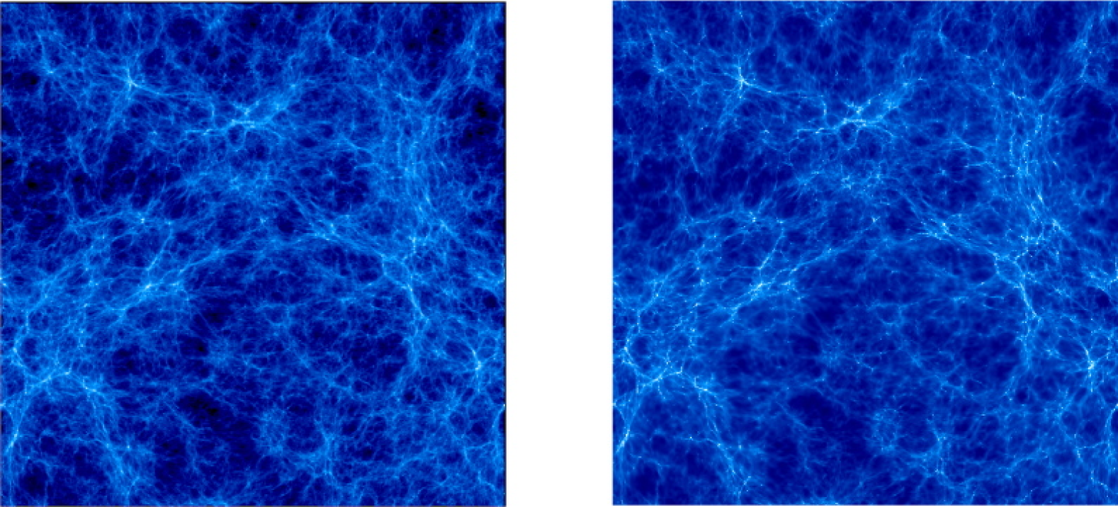
Figure 7.— Comparison between the gas in the SPH MareNostrum simulation at redshift $z=5.7$ (left) from which ICs the Horizon white noise was extracted, and the Horizon-MareNostrum simulation (right) for which the initial conditions were generated with mpgrafic. This figure demonstrates that on large scales the phases are indeed reproduced by the procedure. It also shows that on these scales, the two code produce quite similar features.

The master equation (Eq. (5)) can only be inverted knowing the convolution kernel, i.e. the power spectrum $P(k)$. In principle, the knowledge of the cosmology and the included physics should be sufficient to derive $P(k)$ prior to the deconvolution. Let us call $P_{\mathrm{in}}(k)$, this theoretical power spectrum constrained only by physics. In practice, this theoretical power spectrum differs from the effective power spectrum used to draw the (external, particle based) ICs. Our goal in this section is to define a power spectrum $P_{\mathrm{final}}(k)$ that should accurately represent the ensemble averaged power spectrum of the external ICs (so that $\langle P_{\mathrm{mes}}(k)\rangle\approx P_{\mathrm{final}}(k))$), based on the available theoretical and measured power spectra. $P_{\mathrm{final}}(k)$ will then be used in the deconvolution.

Using an inaccurate spectrum to deconvolve Eq. (5) would lead to a ’colored’ noise for the initial phases, i.e. with spurious characteristic length scales.

Let us illustrate the discrepancy between the theoretical and the measured $P(k)$ by describing the power spectrum of the Mare Nostrum ICs. The measured $P(k)$ is shown in figure 6 as triangles. The theoretical $P(k)=P_{\mathrm{in}}(k)$ (i.e. the one used to generate this set of ICs) is also shown as a dotted line and unsurprisingly, the two curves disagree.

At low $k$, the finite volume of the simulation implies that the empirical power spectrum of large scale modes has large sampling variance and thus departs from the theoretical curve. The high $k$ discrepancy is of different nature: clearly the sampling variance is negligible, but now the discreetness of the grid and anisotropy of very high $k$ mode representation play role. $P(k)$ departs significantly from $P_{\mathrm{in}}(k)$ as easily seen when zooming on the large k regions, where $P(k)$ lacks power compared to the expected behavior. Therefore, $P_{\mathrm{in}}(k)$ cannot be used without corrections to whiten the external IC set. In the following, we rely on the fact that Gaussian initial conditions are statistically characterized by power spectrum only.

The exact set of corrections depends on how the field have been generated. For Mare Nostrum IC’s we must first include a Hanning filter defined in the Fourier space by

$$W_{H}(k)=\cos(\frac{\pi k}{2k_{N}}),$$ (12)

Here the Nyquist frequency is given by $k_{N}=2\pi/L\times N/2$, where $L=50$ Mpc/h is the size of the box of the Mare Nostrum ICs and N stands for the (linear) number of grid elements. Such a filtering is frequently encountered when dealing with initial conditions: because Fourier modes are sampled on a cartesian grid, the two conditions $k<\pi N\sqrt{3}/L$ and $(k_{x},k_{y},k_{z})<\pi N/L$ imply that anisotropies arise on the smallest scales along the diagonals. The Hanning filter damps high frequency modes, and reduces the small scales contributions and consequently the anisotropies. In Fig. 6, we display the $P_{\mathrm{Han}}$ curve as a dashed line, where:

$$P_{\mathrm{Han}}=W_{H}(k)^{2}P_{\mathrm{in}}(k).$$ (13)

Clearly, $P_{\mathrm{Han}}(k)$ reproduces well the measured power spectrum (except at high frequencies, see below), with $N=2048$, which corresponds to the original resolution of the external ICs, prior to some (external) degradation procedure. This modification of the spectrum corresponds to the most favorable case where an analytic expression is known or can be found for the filtering applied on the data.

Secondly, Fig. 6 shows that $P_{\mathrm{Han}}(k)$ still lack some power for $k>40$ h/Mpc. This feature corresponds to the external degradation procedure: one particle out of eight was provided, out of the original $2048^{3}$ particles, resulting in power aliasing at high frequency. This part of the power spectrum was fitted by a smoothed version of the measured power spectrum. We call $P_{\mathrm{final}}(k)$ this final power spectrum that includes the effect of the Hanning Filter and corrects the high frequencies effects due to the degradation:

$$P_{\mathrm{final}}(k)= P_{\mathrm{Han}}(k) \mathrm{k}\leq 40\mathrm{h/Mpc},$$ (14)

$$S[P_{\mathrm{m}es}(k)] \mathrm{k}>40\mathrm{h/Mpc},$$ (15)

where $S[X]$ stands for a smoothing operator. By using a smoothed version of the spectrum, we avoid overfitting of the fluctuations in the spectrum, which would artificially reduce the variance at these scales.

To conclude, $P_{\mathrm{final}}(k)$ combines both an analytic expression of the filtered theoretical spectrum at low frequencies and a numerical evaluation at high frequencies, based on the measured power spectrum. We emphasize that these choices are by no means unique but were found to provide phases with the proper spectrum.

4.1.2 Whitening

The “whitening” operation (i.e. getting the white noise $n_{1}({\bf x})$ from $\delta({\bf x})$ and $P_{\mathrm{final}}(k)$) is then performed by deconvolution as in Eq. (5). For the Horizon Mare Nostrum ICs, the power spectrum of the resulting white noise is shown in Fig. 8. The whitened ICs are now ready to be processed into new initial conditions: the whitened ICs serve as low frequency constraints when generating the refined ICs using mgrafic

Figure 8.— The power spectrum of the phases contained in the ’Mare Nostrum’ initial conditions, with the expectation value of the power of a white noise of unit variance substracted . As expected from a white noise’s realisation, the spectrum fluctuates around an overall flat line.

The code mpgrafic was then used to generate the ICs of a $\Lambda$CDM hydrodynamical “full physics” simulation (with star formation and metals) with a boxsize of $50h^{-1}$Mpc on a grid of $1024^{3}$ using the Horizon reference white noise. The comparison between the input phases and the reproduced phases with mpgrafic is illustrated in Figure 7 which shows both simulations at redshift 5.7.

4.2. Horizon 4$\Pi$

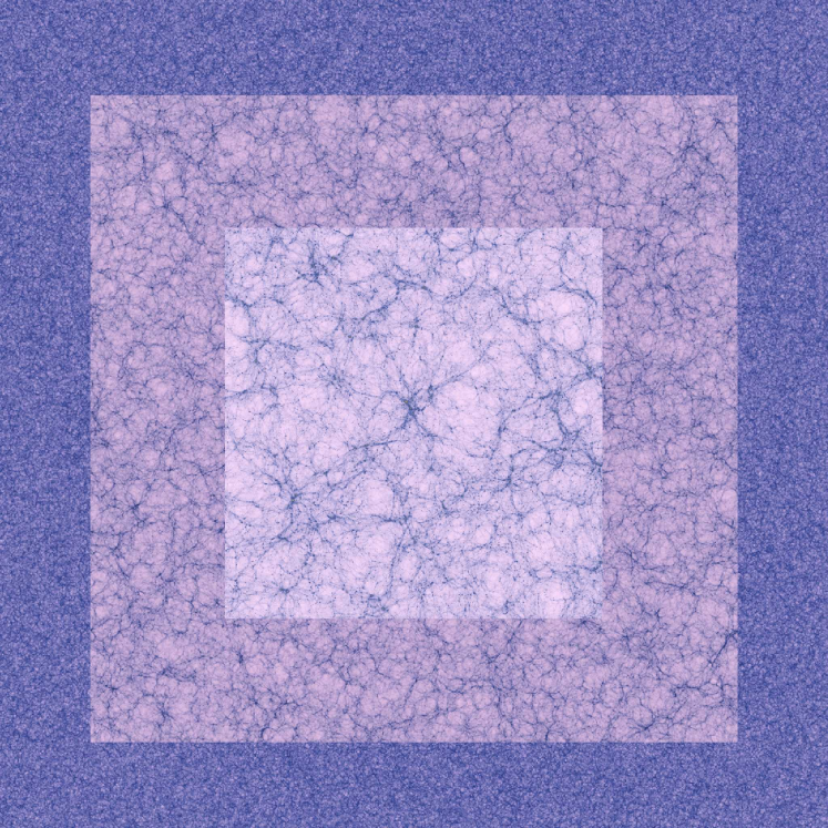
Figure 9.— A multi resolution view of HORIZON 4$\Pi$. The outer region corresponds to a view of the universe on scales of $16h^{-1}$Gpc: it is generated by unfolding the simulation while cuting a slice obliquely through the cube in order to preserve the continuity of the field thanks to the periodicity. The intermediate region corresponds to a slice of $2h^{-1}$Gpc, while the inner region is at the original resolution the initial conditions. RAMSES has refined 6 times over the course of the run from that resolution.

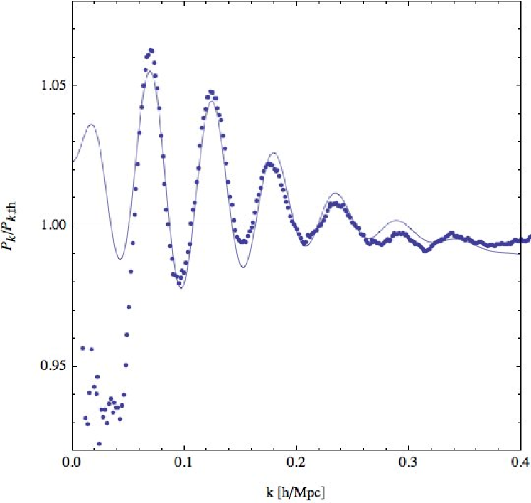
Figure 10.— The measured baryon wiggles at $z=0$ together with the corresponding fit (scaling like $\exp(-[k/0.1]^{1.4})\sin(2\pi k/k_{A})$ plus some linear drift in $k$), which finds that $2\pi/k_{A}=113\>h^{-1}$Mpc.

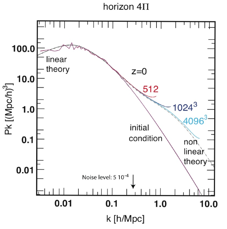
Figure 11.— A Measure of the power spectrum with powergrid of the Horizon-$4\Pi$ in the mpgrafic generated initial condition (bottom curve) and at redshift zero for different samplings (top curves for resp. $512^{3},1024^{3}$and $4096^{3}$ as labeled), with the modes $k$ in units of $h^{-1}$Mpc. Here the density is resampled on the grids using the nearest grid point kernel (NGP) whose bias is corrected. However, the shot noise bias was not corrected in this figure, and no attempt was made to correct the power aliased by the resampling procedure. Both measurements are compared to resp. the linear theory and the theoretical predictions of Smith et al. (2003). Note that the agreement between the linear theory and the generated initial conditions is excellent for all measured scales.

As mentionned earlier, the code mpgrafic was also used to generate the ICs of Horizon-$4\Pi$ a $\Lambda$CDM dark matter only simulation based on cosmological parameters inferred by the WMAP three-years results, with a boxsize of $2h^{-1}$Gpc on a grid of size $4096^{3}$. The purpose of this simulation is to investigate full sky weak lensing and baryonic accoustic oscillations. The 70 billions particles were evolved using the Particle Mesh scheme of the RAMSES code on an adaptively refined grid (AMR) with about 140 billions cells. Each of the 70 billions cells of the base grid was recursively refined up to 6 additional levels of refinement, reaching a formal resolution of 262144 cells in each direction (roughly 7 kpc/h comoving).

The corresponding power spectrum was measured using powergrid, and is shown in Figure 11. Since the simulation snapshots involves a collection of particles, we had to resample them on a grid using a convolution kernel before estimating the power spectrum. The resulting (analytical) bias in the power spectrum was corrected; however, this resampling procedure leads to some power aliasing close to the Nyquist frequency that cannot be corrected without additional information. Finally, note that the AMR structure of the RAMSES code leaves the opportunity of measuring the power spectrum at frequencies beyond the Nyquist frequency of the $4096^{3}$ grid. Such measurements are outside the scope of this paper, and the power spectrum tool powergrid should be viewed primarily as a diagnosis tool. Here, as a check of both the initial condition generation algorithm, including the implementation of the baryon wiggles, a novelty of this implementation, figure 10 displays the measured baryon wiggles in the $z=0$ snapshot, together with the corresponding fit.

5. Conclusion

A series of tools to construct and validate initial conditions for large ($n\geq 1024^{3}$) cosmological simulations in parallel were presented and illustrated. These tools involve ICs generation with optional constraints, low-pass filtering and resampling, power spectrum estimation, estimation of matter density on a grid from a set of particle positions and Peano-Hilbert domain decomposition. As illustrated in section 4, they allowed us to produce very large cosmological simulations. From these high-resolution ICs, one can then create at will, zoom-like initial conditions and constrained ICs with the help of the resampling tool. Let us emphasize that mprafic provides an alternative route to initial condition generation such as Grafic2. It is more versatile as it does not impose any relationship between resolution and boundaries for the refined sub volumes. The remaining limitation is the total amount of memory available on distributed architectures. A logical extension of this work will be to generate initial conditions corresponding to the local group. Note finally that with simple amendments, the above mentionned code could be used in the context of vector field generation (magnetic field with a given helicity), or turbulence.

Appendix A MPgrafics parameter file

Parameters		Description
$4$		Power spectrum parametrization: $4$ is Eisenstein & Hu
$0.24,0.76,73.0$		$\Omega_{m},\Omega_{\Lambda},H_{0}$
$0.042$		$\Omega_{b}$
$0.96$		$n_{S}$
$-0.92$		Normalization: $-\sigma_{8}$ if negative, $Q_{rms}$ if positive
$0.01,100.0$		$k_{min}$ and $k_{max}$ in $h^{-1}Mpc$ for analytical PS output
$-50.0$		Box length in $h^{-1}Mpc$ if negative, mesh length in $Mpc$ if positive
$1$		Grafic1 mode: no choice here
$0$		Grafic1 mode: no choice here
$1$		$1$: Generate noise file and save it / $2$: Read from noise file
$1234$		Initial seed (useful if $1$ is set above)
white-$256$.dat		Noise file name
$1$		$1$: Constraint of large scale phases with small noise file / $2$: No padding
white-$128$.dat		Small (constraint) noise file name

Table 2 mpgrafic parameter file example.

References

- Adelman-McCarthy and for the SDSS Collaboration (2007) J. K. Adelman-McCarthy and for the SDSS Collaboration. The Sixth Data Release of the Sloan Digital Sky Survey. ArXiv e-prints, 707, July 2007.
- Bardeen et al. (1986) J. M. Bardeen, J. R. Bond, N. Kaiser, and A. S. Szalay. The statistics of peaks of gaussian random fields. ApJ, 304:15–61, May 1986.
- Bertschinger (2001) E. Bertschinger. Multiscale Gaussian Random Fields and Their Application to Cosmological Simulations. ApJS, 137:1–20, November 2001.
- Bond et al. (1996) J. R. Bond, L. Kofman, and D. Pogosyan. How filaments of galaxies are woven into the cosmic web. Nature, 380:603–+, April 1996.
- Bond and Myers (1996) J. R. Bond and S. T. Myers. The Peak-Patch Picture of Cosmic Catalogs. I. Algorithms. ApJS, 103:1–+, March 1996.
- Cen and Ostriker (2000) R. Cen and J. P. Ostriker. Physical Bias of Galaxies from Large-Scale Hydrodynamic Simulations. ApJ, 538:83–91, July 2000.
- Eisenstein and Hu (1998) D. J. Eisenstein and W. Hu. Baryonic Features in the Matter Transfer Function. ApJ, 496:605–+, March 1998.
- Frenk et al. (2000) C. S. Frenk, J. M. Colberg, H. M. P. Couchman, G. Efstathiou, A. E. Evrard, A. Jenkins, T. J. MacFarland, B. Moore, J. A. Peacock, F. R. Pearce, P. A. Thomas, S. D. M. White, and N. Yoshida. Public Release of N-body simulation and related data by the Virgo consortium. ArXiv Astrophysics e-prints, July 2000.
- Gottlöber and Yepes (2007) S. Gottlöber and G. Yepes. Shape, Spin, and Baryon Fraction of Clusters in the MareNostrum Universe. ApJ, 664:117–122, July 2007.
- Hoffman and Ribak (1991) Y. Hoffman and E. Ribak. Constrained realizations of Gaussian fields - A simple algorithm. ApJ, 380:L5–L8, October 1991.
- Jarrett et al. (2003) T. H. Jarrett, T. Chester, R. Cutri, S. E. Schneider, and J. P. Huchra. The 2MASS Large Galaxy Atlas. AJ, 125:525–554, February 2003.
- MacNeice et al. (2000) P. MacNeice, K.M. Olson, C. Mobarry, R. de Fainchtein, and C. Packer. PARAMESH: A parallel adaptive mesh refinement community toolkit. Computer Physics Communications, 126(3):330–354, 2000.
- Mohayaee and Tully (2005) R. Mohayaee and R. B. Tully. The Cosmological Mean Density and Its Local Variations Probed by Peculiar Velocities. ApJ, 635:L113–L116, December 2005.
- Ocvirk, Pichon and Teyssier (2008) P. Ocvirk, C. Pichon and R. Teyssier. Bimodal gas accretion in the Mare Nostrum galaxy formation simulation. submitted to MNRAS
- Pen (1997) U.-L. Pen. Generating Cosmological Gaussian Random Fields. ApJ, 490:L127+, December 1997.
- Percival et al. (2001) W. J. Percival, C. M. Baugh, J. Bland-Hawthorn, T. Bridges, R. Cannon, S. Cole, M. Colless, C. Collins, W. Couch, G. Dalton, R. De Propris, S. P. Driver, G. Efstathiou, R. S. Ellis, C. S. Frenk, K. Glazebrook, C. Jackson, O. Lahav, I. Lewis, S. Lumsden, S. Maddox, S. Moody, P. Norberg, J. A. Peacock, B. A. Peterson, W. Sutherland, and K. Taylor. The 2dF Galaxy Redshift Survey: the power spectrum and the matter content of the Universe. MNRAS, 327:1297–1306, November 2001.
- Salmon and Warren (1997) J. Salmon and MS Warren. Parallel, out-of-core methods for N-body simulation. Conference: 8. SIAM conference on parallel processing for scientific computing, Minneapolis, MN (United States), 14-17 Mar 1997, 1997.
- Shirokov (2007) A. Shirokov. GRAvitational COSmology (GRACOS) code release announcement, for version 1.0.1a9. ArXiv e-prints, 711, November 2007.
- Smith et al. (2003) R. E. Smith, J. A. Peacock, A. Jenkins, S. D. M. White, C. S. Frenk, F. R. Pearce, P. A. Thomas, G. Efstathiou, and H. M. P. Couchman. Stable clustering, the halo model and non-linear cosmological power spectra. MNRAS, 341:1311–1332, June 2003.
- Springel et al. (2005) V. Springel, S. D. M. White, A. Jenkins, C. S. Frenk, N. Yoshida, L. Gao, J. Navarro, R. Thacker, D. Croton, J. Helly, J. A. Peacock, S. Cole, P. Thomas, H. Couchman, A. Evrard, J. Colberg, and F. Pearce. Simulations of the formation, evolution and clustering of galaxies and quasars. Nature, 435:629–636, June 2005.
- Teyssier (2002) R. Teyssier. Cosmological hydrodynamics with adaptive mesh refinement. a new high resolution code called ramses. A&A, 385:337–364, April 2002.
- Teyssier et al. (2007) R. Teyssier, S. Pires, D. Aubert, C. Pichon, S. Prunet, A. Amara, K. Benabed, S. Colombi, A. Refregier, J.-L. Starck. Full-Sky Weak Lensing Simulation with 70 Billion Particles. submitted to A&A, 2007.
- van de Weygaert (1996) R. van de Weygaert. Tidal Fields and Structure Formation. In P. Coles, V. Martinez, and M.-J. Pons-Borderia, editors, Mapping, Measuring, and Modelling the Universe, volume 94 of Astronomical Society of the Pacific Conference Series, pages 49–+, 1996.
- Wadsley et al. (2004) J. W. Wadsley, J. Stadel, and T. Quinn. Gasoline: a flexible, parallel implementation of TreeSPH. New Astronomy, 9:137–158, February 2004.
- Weinberg et al. (2002) D. H. Weinberg, L. Hernquist, and N. Katz. High-Redshift Galaxies in Cold Dark Matter Models. ApJ, 571:15–29, May 2002.