Time reversal of Bose-Einstein condensates

Abstract

Using Gross-Pitaevskii equation, we study the time reversibility of Bose-Einstein condensates (BEC) in kicked optical lattices, showing that inside the regime of quantum chaos the dynamics can be inverted from explosion to collapse. The accuracy of time reversal decreases with the increase of atom interactions inside BEC, until it is completely lost. Surprisingly, quantum chaos helps to restore time reversibility. These predictions can be tested with existing experimental setups.

In recent years, there has been remarkable progress in the manipulation and control of the dynamics of BEC in optical lattices (see e.g. the review BECrev ). In such systems, the velocity spreading is very small. This allows to perform very precise investigations of the kicked rotator, known as a paradigm of quantum and classical chaos chirikov . As a result, high order quantum resonances were recently observed experimentally phillips , and various nontrivial effects in the kicked rotator dynamics were probed summy ; auckland . It should be stressed that in BEC the interactions between atoms are of crucial importance, in contrast with other implementations of the kicked rotator with cold atoms raizen ; christensen ; darcy ; garreau , where such interactions are negligible. Recently, a method of time reversal for atomic matter waves has been proposed for the kicked rotator dynamics of noninteracting atoms martin . This method also allows to realize effective cooling of the atoms by a few orders of magnitude. The problem of time reversal of dynamical motion of atoms originates from the famous dispute between Boltzmann and Loschmidt on the origin of irreversible statistical behavior in time reversible systems loschmidt ; boltzmann . The results obtained in martin showed that the quantum dynamics of noninteracting atoms can be reversed in time even if the corresponding classical dynamics is practically irreversible due to dynamical chaos sinai ; lieberman . The investigation of the effect of interactions on time reversibility is of prime importance, since the original dispute between Boltzmann and Loschmidt concerned interacting atoms. In this paper, we study the effects of interactions between atoms in BEC on the time reversal accuracy. We emphasize that interactions bring new elements in the problem of time reversal compared to the case of one particle quantum dynamics martin , acoustic finkac and electromagnetic waves finkem .

To describe the BEC dynamics in a kicked optical lattice we use the Gross-Pitaevskii equation (GPE) pitaev :

$$i\hbar\frac{\partial}{\partial t}\psi=\left(-\frac{\hbar^{2}}{2m}\frac{\partial^{2}}{\partial x^{2}}-g|\psi|^{2}+k\cos x\;\delta_{T}(t)\right)\psi$$ (1)

where the first two terms on the r.h.s. correspond to the usual GPE and the last term represents the effect of the optical lattice, with $\delta_{T}(t)$ being a periodic delta-function with period $T$. The interaction between atoms is quantified by the nonlinearity parameter $g=Ng_{1D}$ where $N$ is the number of atoms in the condensate and $g_{1D}=-2a_{0}\hbar\omega_{\perp}$ is the effective 1D coupling constant, $\omega_{\perp}$ being the radial frequency of the trap and $a_{0}$ the 3D scattering length. Here $\psi(x,t)$ is normalized to one. In the following, we choose units such that $\hbar=m=1$, so that the momentum of atoms is measured in recoil units; time $t$ is measured in units of $T$. For $g=0$ Eq. (1) reduces to the usual kicked rotator model with the classical chaos parameter $K=kT$ and effective Planck constant $T$ (see e.g. martin ). In this case the time reversal can be done in the way described in martin : the forward propagation in time is done with $T=4\pi+\epsilon$ while the backward propagation is performed using $T\rightarrow T^{\prime}=4\pi-\epsilon$, with inversion of the sign of $k$ at the moment of time reversal $t_{r}$. This procedure allows to perform approximate time reversal (ATR) for atoms with small velocities inside the central recoil cell. This ATR procedure works quite accurately for noninteracting atoms ($g=0$), however for real BEC the nonlinear interaction ($g\neq 0$ in (1)) may significantly affect the return probability. Indeed, in the regime of strong interactions and BEC size smaller than the optical lattice period, earlier investigations pikovsky of soliton dynamics in GPE with $g>0$ and periodic boundary conditions showed that with good accuracy a soliton moves along chaotic classical trajectories of the Chirikov standard map chirikov . As a result, even if one performs exact time reversal (ETR), the presence of very small numerical errors completely destroys reversibility due to instability of chaos. However, here we are mainly interested in the regime typical of BEC experiments where the BEC size is larger than the lattice period. Our studies show that in this regime time reversal can be achieved with good accuracy for moderate strength of interactions.

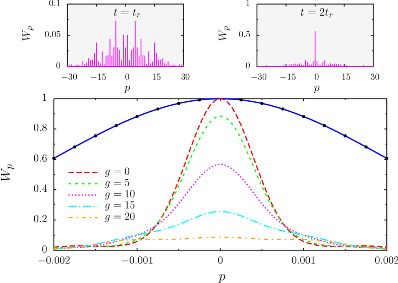
Figure 1: (Color online) Initial (blue/black solid curve) and final return probability distributions $W_{p}$ obtained by ATR procedure vs momentum $p$ for various nonlinearities $g$. Insets : probability distribution $W_{p}$ at $t=t_{r}=10$ (left) and final one at $t=t_{f}=2t_{r}$ (right) on a larger scale for $g=10$. All probability distributions are scaled by their value at $p=0,t=0$. Initial state is a Gaussian packet with rms $\sigma=0.002$. Here $k=4.5$, $T=4\pi+\epsilon$ for $0\leq t\leq t_{r}$ and $T^{\prime}=4\pi-\epsilon$ for $t_{r}<t\leq 2t_{r}$ with $\epsilon=2$ and $t_{r}=10$. Black dots correspond to the wave function after ETR procedure.

To investigate time reversibility for BEC, we numerically simulated the wave function evolution through (1), using up to $N_{s}=2^{23}$ discretized momentum states with $\Delta p=2.5\times 10^{-5}$, space discretization $\Delta x=2\pi/(N_{s}\Delta p)$, and with up to $4\times 10^{4}$ integration time steps between two kicks. In this way we obtain the probability distribution in momentum space $W_{p}(t)=|\langle p|\psi(t)\rangle|^{2}$. The results of time reversal performed by ATR procedure are shown in Fig.1, for an initial Gaussian distribution in momentum with rms $\sigma=0.002$ in recoil units (as in the experiment of phillips ). After this procedure, the returned wave packet at $t=2t_{r}$ becomes clearly squeezed in momentum compared to the initial one. In absence of interactions ($g=0$) the maximum of the final returned distribution $W^{f}_{0}=W_{p=0}(t=2t_{r})$ is equal to the maximum of the initial one $W^{i}_{0}=W_{p=0}(t=0)$ since ATR is exact for $p=0$ martin . The increase of nonlinearity parameter $g$ leads to a reduction of the ratio $W^{f}_{0}/W^{i}_{0}$ until complete destruction of reversibility for $g=20$. However the half-width $p_{L}$ of the returned peak is only weakly affected by $g$. It should be stressed that at the moment of time reversal $t_{r}$ the wave packet is completely destroyed (Fig.1 left inset), and nevertheless the peak is recreated at $t=2t_{r}$ (Fig.1 right inset). This process looks similar to the observed “Bosenova” explosion induced by the change of sign of the interactions in BEC wieman . In our case the sign of interactions is unchanged but the time reversal allows to invert the explosion which happens during $0\leq t\leq t_{r}$ into a collapse for $t_{r}<t\leq 2t_{r}$. We also note that the ETR procedure ($\psi(x)\to\psi^{*}(x)$ at $t=t_{r}$) leads to an almost perfect time reversal of the wave packet, indicating that exponential instability is rather weak on the considered time scales.

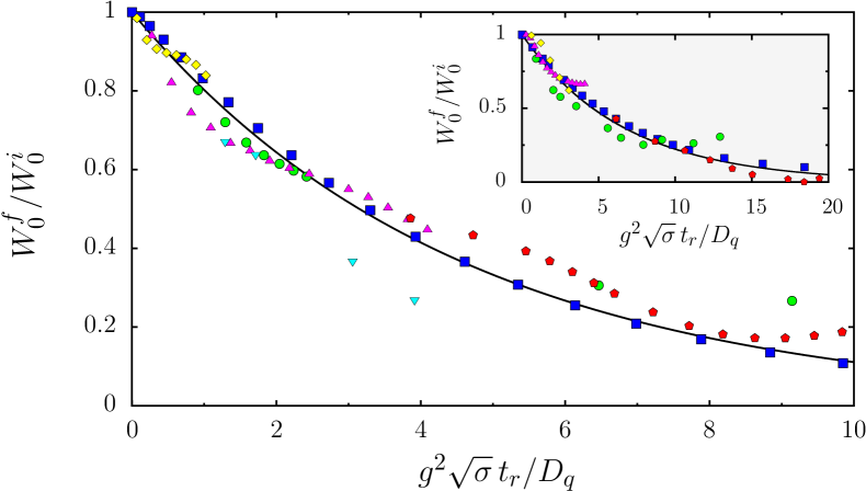
Figure 2: (Color online) Ratio of final to initial probabilities at $p=0$ as a function of $g^{2}\sqrt{\sigma}t_{r}/D_{q}$. Symbols mark the numerical data for: $k=4.5$, $\sigma=0.002$, $t_{r}=10$ ($0\leq g\leq 20$, blue squares); $k=8$, $g=10$, $t_{r}=10$ ($0.002\leq\sigma\leq 0.2$, green circles); $k=4.5$, $g=10$, $\sigma=0.002$ ($1\leq t_{r}\leq 15$, magenta triangles); $g=10$, $\sigma=0.002$, $t_{r}=10$ ($4\leq k\leq 9$, cyan reversed triangles); $k=4.5$, $g=10$ ($g=15$ for the inset), $t_{r}=10$ ($0.002\leq\sigma\leq 0.026$, red pentagons); $k=4.5$, $g=5$ ($g=15$ for the inset), $\sigma=0.002$ ($1\leq t_{r}\leq 15$, yellow diamonds); the curve shows the dependence (2) with $C=0.22$. Inset : same ratio but for a change of sign of $g$ during the reversed evolution, the curve has $C=0.15$.

The dependence of the ratio $W^{f}_{0}/W^{i}_{0}$ on the system parameters is shown in Fig.2. It can be approximately described through

$$W^{f}_{0}/W^{i}_{0}\approx e^{-\Gamma t_{r}}\;,\;\;\;\Gamma=Cg^{2}\sqrt{\sigma}/D_{q}\;,$$ (2)

where $C$ is a numerical constant and $D_{q}$ is the quantum diffusion rate which determines the localization length $l$ of quantum eigenstates in momentum space when $g=0$: $l=D_{q}/2$ with $D_{q}\approx k^{2}/2$ (see exact expression for $D_{q}$ in martin ). Surprisingly enough, the accuracy of time reversal increases with the increase of chaotic diffusion rate $D_{q}$ (see Fig.2). Qualitatively, this is due to the faster spreading of the wave function in coordinate space, that leads to a decrease of the nonlinear term $g|\psi(x,t)|^{2}$ in (1), making the dynamics closer to the linear case for which $W^{f}_{0}=W^{i}_{0}$. An estimate for $\Gamma$ can be obtained assuming that the nonlinear term generates additional corrections $k\rightarrow k+a(t)$ in (1), where $a$ randomly varies in time and $a\sim g|\psi|^{2}\sim g\sigma/\sqrt{l}$. This relation takes into account the normalization condition ($|\psi|^{2}/\sigma\sim 1$) and assumes that inhomogeneities in $|\psi(x)|^{2}$ are smoothed over $l\sim D_{q}$ localized chaotic eigenstates. With these assumptions the decay rate of $W^{f}_{0}/W^{i}_{0}$ is given by the Fermi golden rule $\Gamma\sim|a|^{2}\sim g^{2}\sigma^{2}/D_{q}$. Such a consideration assumes that $\sigma$ remains constant during the dynamics while in fact it increases due to diffusion in momentum that probably leads to the smaller power of $\sigma$ found numerically (2). These estimates qualitatively explain the surprising result of Fig. 2 which shows that the increase of quantum chaos diffusion $D_{q}$ improves the time reversal at fixed $g$.

In addition to the ATR procedure described above, it is possible to perform additionally the inversion of the sign of the interactions $g$ at $t=t_{r}$. In principle such an inversion of $g$ can be realized in experiments similar to those of wieman . The numerical data for this case are shown in the inset of Fig.2. They can be described by the same formula as for the case of unchanged $g$, but with a smaller numerical constant $C$. The relatively small difference between the two cases indicates that the main mechanism of time reversal destruction is related to transitions to other momentum states induced by the nonlinear interaction.

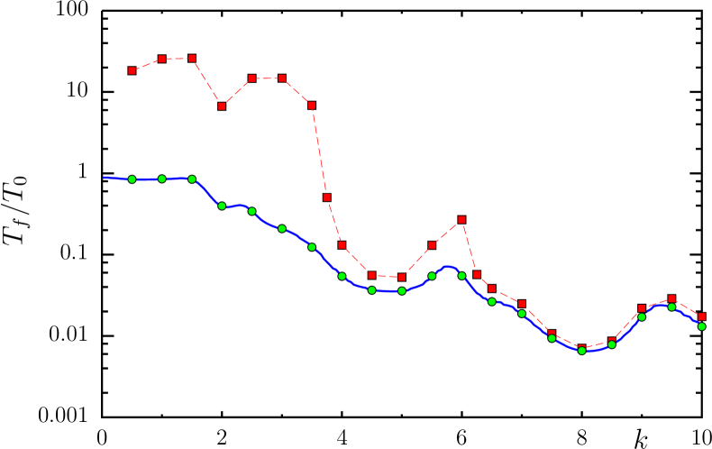
Figure 3: (Color online) Loschmidt cooling of time reversed BEC atoms characterized by the ratio of final $T_{f}$ and initial $T_{0}$ temperatures (solid curve) as a function of $k$ for an initial Gaussian momentum distribution with rms $\sigma=0.002$ and $g=0$ (solid curve), $g=0.5$ (green/gray circles), and $g=10$ (red/black squares). Here $t_{r}=10$ and $\epsilon=2$.

The time reversal leads to a squeezing of the wave packet in momentum space near $p=0$, that can be interpreted as an effective Loschmidt cooling martin . The effect of interactions on this cooling process is analyzed in Fig.3. The temperature $T_{f}$ of the returned atoms can be defined as the temperature of atoms inside the momentum interval $[-2p_{L},2p_{L}]$ at $t=2t_{r}$ (see martin ). For $g=0$, the ratio $T_{f}/T_{0}$ of final and initial temperatures drops significantly with $k$. At small $g=0.5$, the ratio remains essentially unchanged for all values of $k$ considered. In contrast, for stronger nonlinearity ($g=10$), there is no cooling at low values of $k\leq 3$, but for strong chaos with $k>3$ the cooling reappears and becomes very close to the case $g=0$ at large $k$ values. Thus surprisingly strong quantum chaos enhances the cooling of BEC. This result is the consequence of relation (2), according to which the return probability becomes larger and larger with the increase of the quantum diffusion rate $D_{q}\approx k^{2}/2$.

The results presented in Figs.1-3 show that time reversal can be performed for BEC through the ATR procedure even in presence of strong interactions. The cooling mechanism works in presence of these interactions, if the quantum chaos is sufficiently strong.

Up to now we discussed the case of spatial width of BEC much larger than the optical lattice period. It is also interesting to analyze the opposite situation where the BEC size becomes smaller than this period. In this case we start from the soliton distribution

$$\psi(x,t)=\frac{\sqrt{g}}{2}\frac{\exp\left(ip_{0}(x-x_{0}-p_{0}t/2)+ig^{2}t/8\right)}{\cosh\left(\frac{g}{2}(x-x_{0}-p_{0}t)\right)}\;.$$ (3)

For $k=0$ this is the exact solution of Eq.(1), which describes the propagation of a soliton with constant velocity $p_{0}$ refsol . At moderate values of $k$ the shape of the soliton is only slightly perturbed, and its center follows the dynamics described by the Chirikov standard map pikovsky : $\bar{p}_{0}=p_{0}+k\sin x_{0}\;;\;\bar{x}_{0}=x_{0}+\bar{p}_{0}T$, where bars denote the values of the soliton position and velocity after a kick iteration. In the chaotic regime with $K>1$ the soliton dynamics becomes truly chaotic. Indeed, two solitons with slightly different initial velocities or positions diverge exponentially with time. As a result of this instability, even the ETR procedure does not produce an exact return of the soliton to its initial state, due to the presence of numerical integration errors. This is illustrated in Fig.4, where the distance in phase space $\delta$ between initial and returned solitons is shown as a function of the time reversal moment $t_{r}$. If the initial position of the soliton is taken inside the chaotic domain, $\delta$ grows exponentially with $t_{r}$ as $\delta\sim\exp(\lambda t_{r})$. The numerical fit gives a value of $\lambda$ very close to the Kolmogorov-Sinai entropy $h$ of the standard map at the corresponding value of $K$. For large values of $t_{r}$ the values of $\delta$ become so large that the time reversed soliton is located far away from the initial one, and thus time reversibility is completely destroyed (Fig.4 left inset). In contrast, if the soliton starts in the regular domain, the growth of $\delta$ remains weak during the whole integration time. In this regime, even for large values of $t_{r}$ the values of $\delta$ remain small and the soliton returns very close to its initial state (Fig.4 right inset).

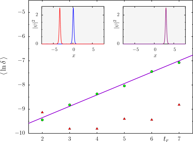
Figure 4: (Color online) Phase space distance $\delta=\sqrt{\delta x^{2}+\delta p^{2}}$ between initial soliton and its time reversed image obtained by ETR ($\psi(x)\to\psi^{*}(x)$) vs $t_{r}$ for $k=1$, $T=2$ and $g=10$; symbols show numerical data averaged over 50 trajectories inside the chaotic (green circles) and the regular (red triangles) domains. The solid line shows the linear fit $\langle\ln\delta\rangle=0.47\,t_{r}-10.29$. The slope is close to the Kolmogorov-Sinai entropy $h\approx 0.45$ at $K=kT=2$. Insets : soliton at initial time $t=0$ (blue/black) and final time $t=2t_{r}$ (red/grey) with $t_{r}=40$ for initial conditions inside the chaotic domain (left) and regular domain (right, initial and final solitons are superimposed).

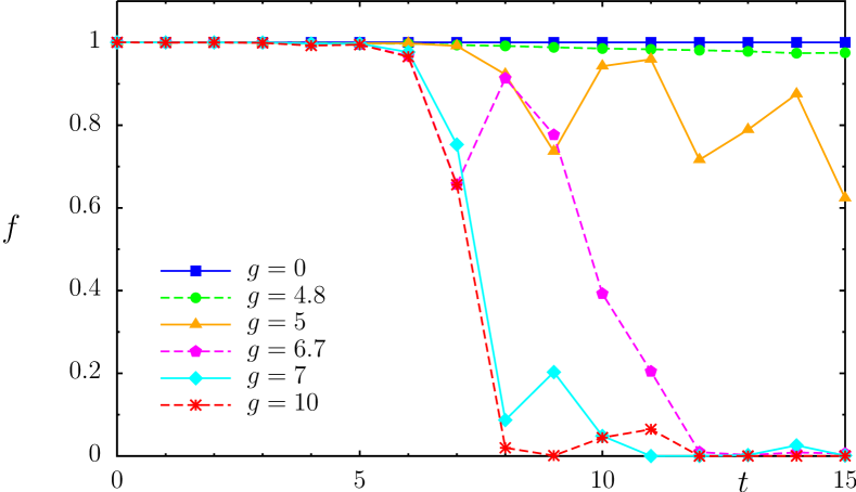
Figure 5: (Color online) Fidelity of two solitons with close initial conditions vs time $t$ for $k=1$, $T=2$ and different nonlinearities. The initial states are solitons (3) with $g=10$ and initial conditions $(x_{0},p_{0})=(0.5,1.25)$ and $(x^{\prime}_{0},p^{\prime}_{0})=(0.5,1.255)$ inside the chaotic domain.

Another way to characterize the stability of nonlinear wave dynamics described by Eq.(1) is to study the behavior of the fidelity defined as $f(t)=|\langle\psi_{1}(t)|\psi_{2}(t)\rangle|^{2}$, where $\psi_{1}$ and $\psi_{2}$ are two solitons with slightly different initial conditions. It is important to note that for $g=0$ the function $f(t)$ is independent of $t$, thus variation with time appears only due to nonlinear effects. In a certain sense this quantity can be considered as a generalization of the usual fidelity prosen discussed for the Schrödinger evolution to the case of nonlinear evolution given by GPE. The dependence of $f$ on time is shown in Fig.5 for different values of the nonlinearity parameter $g$. For small values of $g$ the function is almost constant on the considered time interval, while for large values of $g$ it drops quickly to almost zero after a logarithmically short time scale corresponding to the separation of the two solitons. These two qualitatively different behaviors can be understood as follows. For relatively weak nonlinearity, $f(t)\sim\exp(-\Gamma t)$ with $\Gamma\propto g^{2}$ (see Eq.(2)) that corresponds to the usual Fermi golden rule regime of the fidelity decay in linear quantum systems with perturbation prosen . For stronger $g$, we enter the regime where nonlinear wave packets move like chaotic individual particles that leads to an abrupt drop of fidelity as soon as the separation becomes larger than the size of wave packets. In this regime the size of BEC is smaller than the lattice period and the time reversal is destroyed. In the opposite limit of large BEC size shown in Fig. 1 the time reversal can be maintained at moderate values of $g$. The transition between these two regimes is rather nontrivial and requires further investigations.

The results of Figs.4-5 show that the soliton dynamics described by GPE (1) is truly chaotic. This leads to the destruction of time reversibility induced by exponential growth of small perturbations. However, the real BEC is a quantum object with a mass proportional to the number of atoms $N$. Thus it has effective $\hbar_{\mathrm{eff}}\propto 1/\sqrt{N}$ and since the Ehrenfest time $t_{E}$ for chaotic dynamics depends only logarithmically on $\hbar$ chirikov ; prosen this time remains rather short $t_{E}\sim|\ln\hbar_{\mathrm{eff}}|/h\sim(\ln N)/2h$. Thus for conditions of Fig.4 and $N=10^{5}$ we have $t_{E}\approx 13$ and on larger times quantum BEC should have no exponential instability of motion. Hence, in the time reversal procedure the real quantum BEC remains stable and reversible contrary to the BEC described by GPE. We think that the resolution of this paradox relies on the absence of second quantization in GPE that makes the soliton dynamics essentially classical.

The dimensionless nonlinear parameter is $g=-Na_{0}\lambda/2\pi l_{\perp}^{2}$, where $l_{\perp}=\sqrt{\hbar/m\omega_{\perp}}$ and $2\lambda$ is the optical lattice period. Values of $g\approx 0.1$ have been achieved at radial frequency $800$Hz and $N\approx 5000\approx N_{max}=l_{\perp}/|a_{0}|$hulet . This value can be further increased up to $g\approx 10$ by increasing $\omega_{\perp}$ (e.g. $20$ kHz hinds ) and increasing $\lambda$ using a CO₂-laser hansch or tilted laser beams. Thus experimental setups similar to phillips ; summy ; auckland ; hulet can test the fundamental question of BEC time reversal discussed here.

We thank CalMiP for access to their supercomputers and the French ANR (project INFOSYSQQ) and the EC project EuroSQIP for support.

References

- (1) O. Morsch and M. Oberthaler, Rev. Mod. Phys. 78, 179 (2006).
- (2) B. V. Chirikov, Phys. Rep. 52, 263 (1979); B. V. Chirikov et al., Sov. Scient. Rev. C 2, 209 (1981); Physica 33D, 77 (1988); B. Chirikov and D. Shepelyansky, Scholarpedia 3(3):3550 (2008).
- (3) C. Ryu et al., Phys. Rev. Lett. 96, 160403 (2006).
- (4) G. Behinaein et al., Phys. Rev. Lett. 97, 244101 (2006).
- (5) S. A. Wayper et al., Europhys. Lett. 79, 60006 (2007).
- (6) F. L. Moore et al., Phys. Rev. Lett. 75, 4598 (1995).
- (7) H. Ammann et al., Phys. Rev. Lett. 80, 4111 (1998).
- (8) S. Schlunk et al., Phys. Rev. Lett. 90, 124102 (2003).
- (9) J. Chabé et al., preprint arXiv:0709.4320 (2007).
- (10) J. Martin et al., Phys. Rev. Lett. 100, 044106 (2008).
- (11) J. Loschmidt, Sitzungsberichte der Akademie der Wissenschaften, Wien, II, 73, 128 (1876).
- (12) L. Boltzmann, Sitzungsberichte der Akademie der Wissenschaften, Wien, II, 75, 67 (1877).
- (13) I. P. Kornfeld et al., Ergodic theory, Springer, N.Y., (1982).
- (14) A. Lichtenberg and M. Lieberman, Regular and Chaotic Dynamics, Springer, N.Y. (1992).
- (15) A. Derode et al., Phys. Rev. Lett. 75, 4206 (1995); J. de Rosny et al., ibid. 84, 1693 (2000).
- (16) G. Lerosey et al., Phys. Rev. Lett. 92, 193904 (2004); Science 315, 1120 (2007).
- (17) F. Dalfovo et al., Rev. Mod. Phys. 71, 463 (1999).
- (18) F. Benvenuto et al., Phys. Rev. A 44, R3423 (1991).
- (19) E. A. Donley et al., Nature 412, 295 (2001).
- (20) V. E. Zakharov and A.B. Shabat, Sov. Phys. JETP 34, 62 (1972) [Zh. Eks. Teor. Fiz. 61, 118 (1971)].
- (21) T. Gorin et al., Phys. Rep. 435, 33 (2006).
- (22) K. E. Strecker et al., Nature 417, 150 (2002).
- (23) I. Llorente-Garcia et al., J. Phys. Conf. Ser. 19, 70 (2005).
- (24) S. Friebel et al., Phys. Rev. A 57, R20 (1998).