http://www-fourier.ujf-grenoble.fr/ bkloeckn/ \normalparindent\normalparindent\normalparindent\normalparindent\normalparindent\listisep\normalparindent\normalparindent
A geometric study of Wasserstein spaces:
Euclidean spaces
Abstract
In this article we consider Wasserstein spaces (with quadratic transportation cost) as intrinsic metric spaces. We are interested in usual geometric properties: curvature, rank and isometry group, mostly in the case of Euclidean spaces. Our most striking result is that the Wasserstein space of the line admits “exotic” isometries, which do not preserve the shape of measures.
Key words and phrases:
Wasserstein distance, optimal transportation, isometries, rank1991 Mathematics Subject Classification:
54E70, 28A331. Introduction
The concept of optimal transportation recently raised a growing interest in links with the geometry of metric spaces. In particular the Wasserstein space have been used by Von Renesse and Sturm [15], Sturm [17] and Lott and Villani [12] to define certain curvature conditions on a metric space . Many useful properties are inherited from by (separability, completeness, geodesicness, some non-negative curvature conditions) while some other are not, like local compacity.
In this paper, we study the geometry of Wasserstein spaces as intrinsic spaces. We are interested, for example, in the isometry group of , in its curvature and in its rank (the greatest possible dimension of a Euclidean space that embeds in it). In the case of the Wasserstein space of a Riemannian manifold, itself seen as an infinite-dimensional Riemannian manifold, the Riemannian connection and curvature have been computed by Lott [13]. See also [18] where Takatsu studies the subspace of Gaussian measures in , and [1] where Ambrosio and Gigli are interested in the second order analysis on , in particular its parallel transport.
The Wasserstein space contains a copy of , the image of the isometric embedding
where is the Dirac mass at . Moreover, given an isometry of one defines an isometry of by . We thus get an embedding
These two elementary facts connect the geometry of to that of .
One could expect that is onto, i.e. that all isometries of are induced by those of itself. Elements of are called trivial isometries. Let us introduce a weaker property: a self-map of is said to preserve shapes if for all , there is an isometry of (that depends upon ) such that . An isometry that does not preserve shapes is said to be exotic.
Our main result is the surprising fact that admits exotic isometries. More precisely we prove the following.
\theoname \the\smf@thm.
The isometry group of is a semidirect product
| (1) |
Both factors decompose: and the action defining the semidirect product (1) is simply given by the usual action of the left factor on the right factor, that is where is identified with .
In (1), the left factor is the image of and the right factor consist in all isometries that fix pointwise the set of Dirac masses. In the decomposition of the latter, the factor is generated by a non-trivial involution that preserves shapes, while the factor is a flow of exotic isometries.
The main tool we use is the explicit description of the geodesic between two points , of that follows from the fact that the unique optimal transportation plan between and is the non-decreasing rearrangement. It implies that most of the geodesics in are not complete, and we rely on this fact to give a metric characterization of Dirac masses and of linear combinations of two Dirac masses, among all points of . We also use the fact that has vanishing curvature in the sense of Alexandrov.
Let us describe roughly the non-trivial isometries that fix pointwise the set of Dirac masses. On the one hand, the non-trivial isometry generating the factor is defined as follows: a measure is mapped to its symmetric with respect to its center of mass. On the other hand, the exotic isometric flow tends to put all the mass on one side of the center of gravity (that must be preserved), close to it, and to send a small bit of mass far away on the other side (so that the Wasserstein distance to the center of mass is preserved). In particular, under this flow any measure converges weakly (but of course not in ) to (where is the center of mass of ), see Proposition 5.2.
The case of the line seems very special. For example, admits non-trivial isometries but all of them preserve shapes.
\theoname \the\smf@thm.
If , the isometry group of is a semidirect product
| (2) |
where the action of an element on is the conjugacy by its linear part .
The left factor is the image of and each element in the right factor fixes all Dirac masses and preserves shapes.
The proof relies on Theorem 1, some elementary properties of optimal transportation in and Radon’s Theorem [14].
We see that the quotient is compact if and only if . The higher-dimensional Euclidean spaces are more rigid than the line for this problem, and we expect most of the other metric spaces to be even more rigid in the sense that is onto.
Another consequence of the study of complete geodesics concerns the rank of .
\theoname \the\smf@thm.
There is no isometric embedding of into .
It is simple to prove that despite Theorem 1, large pieces of can be embedded into , which has consequently infinite weak rank in a sense to be precised. As a consequence, we get for example:
\propname \the\smf@thm.
If is any Polish geodesic metric space that contains a complete geodesic, then is not -hyperbolic.
This is not surprising, since it is well-known that the negative curvature assumptions tend not to be inherited from by its Wasserstein space. An explicit example is computed in [2] (Example 7.3.3); more generaly, if contains a rhombus (four distinct points so that is independent of the cyclic index ) then is not uniquely geodesic, and in particular not , even if itself is strongly negatively curved.
Organization of the paper
Acknowledgements
I wish to thank all speakers of the workshop on optimal transportation held in the Institut Fourier in Grenoble, especially Nicolas Juillet with whom I had numerous discussion on Wasserstein spaces, and its organizer Hervé Pajot. I am also indebted to Yann Ollivier for advises and pointing out some inaccuracies and mistakes in preliminary versions of this paper.
2. The Wasserstein space
In this preliminary section we recall well-known general facts on . One can refer to [19, 20] for further details and much more. Note that the denomination “Wasserstein space” is debated and historically inaccurate. However, it is now the most common denomination and thus an occurrence of the self-applying theorem of Arnol’d according to which a mathematical result or object is usually attributed to someone that had little to do with it.
2.1. Geodesic spaces
Let be a Polish (i.e. complete and separable metric) space, and assume that is geodesic, that is: between two points there is a rectifiable curve whose length is the distance between the considered points. Note that we only consider globally minimizing geodesics, and that a geodesic is always assumed to be parametrized proportionally to arc length.
One defines the Wasserstein space of as the set of Borel probability measures on that satisfy
for some (hence all) point , equipped by the distance defined by:
where the infimum is taken over all coupling of , . A coupling realizing this infimum is said to be optimal, and there always exists an optimal coupling.
The idea behind this distance is linked to the Monge-Kantorovitch problem: given a unit quantity of goods distributed in according to , what is the most economical way to displace them so that they end up distributed according to , when the cost to move a unit of good from to is given by ? The minimal cost is and a transportation plan achieving this minimum is an optimal coupling.
An optimal coupling is said to be deterministic if it can be written under the form where is a measurable map and is if is satisfied and otherwise. This means that the coupling does not split mass: all the mass at point is moved to the point . One usually write . Of course, for to be a coupling between and , the relation must hold.
Under the assumptions we put on , the metric space is itself Polish and geodesic. If moreover is uniquely geodesic, then to each optimal coupling between and is associated a unique geodesic in in the following way. Let be the set of continuous curves , let be the application that maps to the constant speed geodesic between these points, and for each let be the map . Then is a geodesic between and . Informally, this means that we choose randomly a couple according to the joint law , then take the time of the geodesic . This gives a random point in , whose law is , the time of the geodesic in associated to the optimal coupling . Moreover, all geodesics are obtained that way.
Note that for most spaces , the optimal coupling is not unique for all pairs of probability measures, and is therefore not uniquely geodesic even if is.
One of our goal is to determine whether the Dirac measures can be detected inside by purely geometric properties, so that we can link the isometries of to those of .
2.2. The line
Given the distribution function
of a probability measure , one defines its left-continuous inverse:
that is a non-decreasing, left-continuous function; is the infimum of the support of and its supremum. A discontinuity of happens for each interval that does not intersect the support of , and is constant on an interval for each atom of .
Let and be two points of , and let be their distribution functions. Then the distance between and is given by
| (3) |
and there is a unique constant speed geodesic , where has a distribution function defined by
| (4) |
This means that the best way to go from to is simply to rearrange increasingly the mass, a consequence of the convexity of the cost function. For example, if and are uniform measures on and , then the optimal coupling is deterministic given by the translation . That is: the best way to go from to is to shift every bit of mass by . If the cost function where linear, it would be equivalent to leave the mass on where it is and move the remainder from to . If the cost function where concave, then the latter solution would be better than the former.
2.3. Higher dimensional Euclidean spaces
The Monge-Kantorovich problem is far more intricate in () than in . The major contributions of Knott and Smith [11, 16] and Brenier [3, 4] give a quite satisfactory characterization of optimal couplings and their unicity when the two considered measures and are absolutely continuous (with respect to the Lebesgue measure). We shall not give details of these works, for which we refer to [19, 20] again. Let us however consider some toy cases, which will prove useful later on. Missing proofs can be found in [10], Section 2.1.2.
We consider endowed with its canonical inner product and norm, denoted by .
Translations
Let be the translation of vector and assume that . Then the unique optimal coupling between and is deterministic, equal to , and therefore . This means that the only most economic way to move the mass from to is to translate each bit of mass by the vector . This is a quite intuitive consequence of the convexity of the cost. In particular, the geodesic between and can be extended for all times . This happens only in this case as we shall see later on.
Dilations
Let be the dilation of center and ratio and assume that . Then the unique optimal coupling between and is deterministic, equal to . In particular,
As a consequence, the geodesic between and is unique and made of homothetic of , and can be extended only to a semi-infinite interval: it cannot be extended beyond (unless is a Dirac mass itself).
Orthogonal measures
Assume that and are supported on orthogonal affine subspaces and of . Then if is any coupling, assuming , we have
therefore the cost is the same whatever the coupling.
Balanced combinations of two Dirac masses
Assume that and . A coupling between and is entirely determined by the amount of mass sent from to . The cost of the coupling is
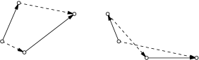
thus the optimal coupling is unique and deterministic if , given by the map if and by the map if (figure 3). Of course if , then all coupling have the same cost and are therefore optimal.
If the combinations are not balanced (the mass is not equally split between the two point of the support), then the optimal coupling is easy to deduce from the preceding computation. For example if then as much mass as possible must be sent from to , and this determines the optimal coupling.
This example has a much more general impact than it might seem: it can be generalized to the following (very) special case of the cyclical monotonicity (see for example [20], Chapter 5) which will prove useful in the sequel.
\lemmname \the\smf@thm.
If is an optimal coupling between any two probability measures on , then
holds whenever and are in the support of .
2.4. Spaces of nonpositive curvature
In this paper we shall consider two curvature conditions. The first one is a negative curvature condition, the -hyperbolicity introduced by Gromov (see for example [5]). A geodesic space is said to be -hyperbolic (where is a non-negative number) if in any triangle, any point of any of the sides is at distance at most from one of the other two sides. For example, the real hyperbolic space is -hyperbolic (the value of depending on the value of the curvature), a tree is -hyperbolic and the euclidean spaces of dimension at least are not -hyperbolic for any .
The second condition is the classical non-positive sectional curvature condition , detailed in Section 4, that roughly means that triangles are thinner in than in the euclidean plane. Euclidean spaces, any Riemannian manifold having non-positive sectional curvature are examples of locally spaces.
A geodesic Polish space is also called a Hadamard space. A Hadamard space is uniquely geodesic, and admits a natural boundary at infinity. The feature that interests us most is the following classical result: if is a Hadamard space, given there is a unique point , called the center of mass of , that minimizes the quantity . If is endowed with the canonical scalar product, then the center of mass is of course but in the general case, the lack of an affine structure on prevents the use of such a formula.
We thus get a map that maps any probability measure to its center of mass. Obviously, is a left inverse to and one can hope to use this map to link closer the geometry of to that of . That’s why our questions, unlike most of the classical ones in optimal transportation, might behave more nicely when the curvature is non-positive than when it is non-negative.
3. Geodesics
The content of this section, although difficult to locate in the bibliography, is part of the folklore and does not pretend to originality. We give proofs for the sake of completeness.
3.1. Case of the line
We now consider the geodesics of . Our first goal is to determine on which maximal interval they can be extended.
Maximal extension
Let , be two points of and , their distribution functions. Let be the geodesic between and . Since is uniquely geodesic, there is a unique maximal interval on which can be extended into a geodesic, denoted by .
\lemmname \the\smf@thm.
One has
where is defined by the formula (4). It is a closed interval. If one of its bound is finite, then does not have bounded density with respect to the Lebesgue measure.
Proof.
Any non-decreasing left continuous function is the inverse distribution function of some probability measure. If such a function is obtained by an affine combination of probabilities belonging to , then its probability measure belongs to too.
Moreover, an affine combination of two left continuous function is left continuous, so that
The fact that is closed follows from the stability of non-decreasing functions under pointwise convergence.
If the minimal slope
is positive for some , then it stays positive in a neighborhood of . Thus, a finite bound of must have zero minimal slope, and cannot have a bounded density. ∎
A geodesic is said to be complete if it is defined for all times. We also consider geodesic rays, defined on an interval or (in the latter case we say that the ray is complete), and geodesic segments, defined on a closed interval.
It is easy to deduce a number of consequences from Lemma 3.1.
\propname \the\smf@thm.
In :
-
(1)
any geodesic ray issued from a Dirac mass can be extended to a complete ray,
-
(2)
no geodesic ray issued from a Dirac mass can be extended for negative times, except if all of its points are Dirac masses,
-
(3)
up to normalizing the speed, the only complete geodesics are those obtained by translating a point of :
Proof.
The inverse distribution function of a Dirac mass is the constant function with value . Since it slopes
are all zero, for all positive times the functions defined by formula (4) for any non-decreasing are non-decreasing. However, for the are not non-decreasing if is not constant, we thus get (1) and (2).
Consider a point of defined by an inverse distribution function , and consider a complete geodesic issued from . Let be the inverse distribution function of . Then, since is defined for all times , the slopes of must be greater than those of :
otherwise, when increases, some slope of will decrease linearly in , thus becoming negative in finite time.
But since is also defined for all , the slopes of must be lesser than those of . They are therefore equal, and the two inverse distribution function are equal up to an additive constant. The geodesic is the translation of and we proved (3). ∎
Convex hulls of totally atomic measures
Define in the following sets:
Recall that if is a Polish geodesic space and is a subset of , one says that is convex if every geodesic segment whose endpoints are in lies entirely in . The convex hull of a subset is the least convex set that contains . It is well defined since the intersection of two convex sets is a convex set, and is equal to where and is obtained by adding to all points lying on a geodesic whose endpoints are in .
Since is the image of the isometric embedding , it is a convex set. This is not the case of is . In fact, we have the following.
\propname \the\smf@thm.
If , any point of lies on a geodesic segment with endpoints in . Moreover, the endpoints can be chosen with the same center of mass than that of .
Proof.
If the result is obvious. Assume is in . We can assume further that . Consider the measures
Then lies on the geodesic segment from to . To get a constant center of mass, one considers the geodesic
where . ∎
In particular, we get the following noteworthy fact that will prove useful latter on.
\propname \the\smf@thm.
The convex hull of is dense in if .
Proof.
Follows from Proposition 3.1 since the set of totally atomic measures is dense in . ∎
3.2. Complete geodesics in higher dimension
In , the optimal coupling and thus the geodesics are not as explicit as in the case of the line. It is however possible to determine which geodesic can be extended to all times in .
\lemmname \the\smf@thm.
Let be a geodesic in associated to an optimal coupling between and . Then for all times and in and all pair of points in the support of , the following hold:
where and .
Proof.
Let us introduce the following notations: for all pair of points , and is the law of the random variable where is any random variable of law . As we already said, is an optimal coupling of whose corresponding geodesic is the restriction of to .
Since is optimal, according to the cyclical monotonicity (see Lemma 2.3) one has .
But with the above notations, one has and , and we get the desired inequality. ∎
Let us show why this Lemma implies that the only complete geodesics are those obtained by translation. There are immediate consequences on the rank of , see Theorem 1 and Section 7.
\propname \the\smf@thm.
Let be a geodesic in defined for all times. Then there is a vector such that .
This result holds even if , as stated in Proposition 3.1.
Proof.
It is sufficient to find a such that , since then there is only one geodesic from to .
Consider any pair of points in the support of the coupling between and that defines the restriction of to . Define and . If , then there are real numbers such that . Then the coupling between and that defines the restriction of to , defined as above, cannot be optimal. This is a contradiction with the assumption that is a geodesic.
Therefore, for all in the support of one has . This amounts to say that is deterministic, given by a translation of vector . ∎
4. Curvature
Once again, this section mainly collects some facts that are already well-known but shall be used on the sequel.
More details on the (sectional) curvature of metric spaces are available for example in [6] or [9]. We shall consider the curvature of , in the sense of Alexandrov. Given any three points in a geodesic metric space , there is up to congruence a unique comparison triangle in , that is a triangle that satisfies , , and .
One says that has non-positive curvature (in the sense of Alexandrov), or is , if for all the distances between two points on sides of this triangle is lesser than or equal to the distance between the corresponding points in the comparison triangle, see figure 4.
Equivalently, is if for any triangle , any geodesic such that and , and any , the following inequality holds:
| (5) |
where denotes the length of , that is .
One says that has vanishing curvature if equality holds for all :
| (6) |
This is equivalent to the condition that for any triangle in and any point on any geodesic segment between and , the distance between and is equal to the corresponding distance in the comparison triangle.
\propname \the\smf@thm.
The space has vanishing Alexandrov curvature.
Proof.
It follows from the expression (3) of the distance in : if we denote by the inverse distribution functions of the three considered points , we get:
and using that and ,
∎
We shall use the vanishing curvature of by means of the following result, where all subsets of are assumed to be endowed with the induced metric (that need therefore not be inner).
\propname \the\smf@thm.
Let be a Polish uniquely geodesic space with vanishing curvature. If is a subset of and is the convex hull of , then any isometry of can be extended into an isometry of .
Proof.
Let the isometry to be extended. Let be any points lying each on one geodesic segment whose endpoints are in . Consider the unique geodesics that satisfy , , and the points , lying on them so that , , and the same for . This makes sense since, being an isometry on , has the length of and that of . We shall prove that .
The vanishing of curvature implies that : the triangles and have the same comparison triangle. Similarly . Now and have the same comparison triangle, and the vanishing curvature assumption implies .
In particular, if then . We can thus extend to the union of geodesic segments whose endpoints are in by mapping any such to the corresponding . This is well-defined, and an isometry. Repeating this operation we can extend into an isometry of . But being complete, the continuous extension of to is well-defined and an isometry. ∎
Note that the same result holds with the same proof when the curvature is constant but non-zero.
Higher dimensional case
Proposition 4 does not hold in . In effect, there are pairs of geodesics that meet at both endpoints (take measures whose support lie on orthogonal subspaces of ). Taking a third point in one of the two geodesics, one gets a triangle in whose comparison triangle has its three vertices on a line. This implies that is not . The situation is in fact worse than that: in any neighborhood of any point of one can find two different geodesics that meet at their endpoints. One can say that this space has positive sectional curvature at arbitrarily small scales.
5. Isometries: the case of the line
5.1. Existence and unicity of the non-trivial isometric flow
In this section, we prove Theorem 1.
Let us start with the following consequence of Proposition 3.1.
\lemmname \the\smf@thm.
An isometry of must globally preserve the sets and .
Proof.
We shall exhibit some geometric properties that characterize the points of and and must be preserved by isometries.
First, according to Proposition 3.1, the points are the only ones to satisfy: every maximal geodesic ray starting at is complete. Since an isometry must map a geodesic (ray, segment) to another, this property is preserved by isometries of .
Second, let us prove that the point are the only ones that satisfy: any geodesic such that and that can be extended to a maximal interval with , has its endpoint in .
This property is obviously satisfied by points of . It is also satisfied by every points of . Indeed, denote by the distribution function of and write where . Then if does not write with , either
-
•
there are two reals such that and ,
-
•
there are two reals such that and , or
-
•
is a Dirac mass.
In the first two cases, is not defined for , and in the third one, it is not defined for . If does write , then either and is defined for all , or and is only defined until a finite positive time, or and is defined from a finite negative time where .
Now if , its inverse distribution function takes three different values at some points . Consider the geodesic between and the measure whose inverse distribution function coincide with on but is defined by
on (see figure 6). Then this geodesic is defined for all positive times, but stops at some nonpositive time . Since takes different values at and , one can extend the geodesic for small negative times and . But the inverse distribution function of the endpoint must take the same values than that of in and , thus . ∎
Now we consider isometries of , to which all isometries of shall be reduced.
Any point writes under the form
where is its center of mass, is the distance between and its center of mass, and is any real number. In probabilistic terms, if is the law of a random variable then is its expected value and its variance.
\lemmname \the\smf@thm.
An isometry of that fixes each point of must restrict to to a map of the form:
for some . Any such map is an isometry of .
Proof.
Let be an isometry of that fixes each point of .
A computation gives the following expression for the distance between two measures in :
Since is an isometry, it preserves the center of mass and variance. The preceding expression shows that it must preserve the euclidean distance between and for any two measures , and that this condition is sufficient to make an isometry of . ∎
\lemmname \the\smf@thm.
Let and be isometries of . Then
Proof.
It follows from a direct computation:
∎
We are now able to prove our main result.
Proof of Theorem 1.
First Lemma 5.1 says that any isometry of acts on and .
Let be and be the subset of consisting of isometries that fix pointwise. Then is a normal subgroup of .
Let be an isometry of . It acts isometrically on , thus there is an isometry of such that . In particular, . Since is reduced to the identity, we do have a semidirect product .
According to Proposition 4, each map extends into an isometry of , which is by Proposition 3.1. We still denote by this extension. Proposition 3.1 also shows that an isometry of is entirely determined by its action on . The description of now follows from Lemma 5.1.
If denotes the symmetry around , then maps a measure to its symmetric with respect to its center of mass, thus preserves shapes. Any other is a translation or the composition of and a translation.
By the exotic isometry flow of we mean the flow of isometries obtained when is a translation. This flow does not preserve shapes as is seen from its expression in .
At last, Lemma 5.1 gives the asserted description of the semidirect product. ∎
5.2. Behaviour of the exotic isometry flow
The definition of is constructive, but not very explicit outside . On , the flow tends to put most of the mass on the right of the center of mass, very close to it, and send a smaller and smaller bit of mass far away on the left.
The flow preserves as its elements are the only ones to lie on a geodesic segment having both endpoints in . Similarly, elements of are the only ones to lie on a geodesic segment having an endpoint in and another in , therefore preserves for all .
Direct computations enable one to find formulas for on , but the expressions one gets are not so nice. For example, if where , then
In order to get some intuition about , let us prove the following.
\propname \the\smf@thm.
Let be any point of and its center of mass. If goes to , then converges weakly to .
Proof.
We shall only consider the case when since the other one is symmetric. Let us start with a lemma.
\lemmname \the\smf@thm.
If and are in and both converge weakly to when goes to , and if is in the geodesic segment between and for all , then converges weakly to when goes to .
Proof.
It is a direct consequence of the form of geodesics: if and both charge an interval with a mass at least , then must charge this interval with a mass at least . ∎
Now we are able to prove the proposition on larger and larger subsets of . First, it is obvious on . If it holds on , the preceding Lemma together with Proposition 3.1 implies that it holds on . To prove it on the whole of , the density of the subset of consisting of measures having center of mass , and a diagonal process are sufficient. ∎
6. Isometries: the higher-dimensional case
To show that the exotic isometry flow of is exceptional, let us consider the higher-dimensional case : there are isometries of that fix pointwise the set of Dirac masses, but there are not so many and they preserve shapes.
6.1. Existence of non-trivial isometries
We start with the existence of non-trivial isometries, that however preserves shapes.
\propname \the\smf@thm.
If is a linear isometry of , then the map
where denotes both the center of mass of and the corresponding translation, is an isometry of (see figure 8).

Note that we need to be linear, thus we do not get as many non-trivial isometries as in . Moreover, all isometries constructed this way preserve shapes.
Proof.
We only need to check the case of absolutely continuous measures since they form a dense subset of . In that case, there is a unique optimal coupling that is deterministic, given by a map such that . Denote by and the centers of mass of and . Let us show that there is a good coupling between and .
Let be the map defined by
By construction . Moreover the cost of the coupling is
This shows that and are at distance at most . Applying the same reasoning to , we get that and is an isometry. ∎
6.2. Semidirect product decomposition
The Dirac masses are the only measures such that any geodesic issued from them can be extended for all times (given any other measure, the geodesic pointing to any Dirac mass cannot be extended past it, see in Section 2.3 the paragraph on dilations). As a consequence, an isometry of must globally preserve the set of Dirac masses
As in the case of the line, if we let and be the set of isometries of that fix each Dirac mass, then . We proved above that contains a copy of , and is in particular non-trivial.
Moreover, if one conjugates a by some , where and , one gets the map (it is sufficient to check this on some measure in the easy cases when is a translation or fixes the center of mass of ). Therefore, the action of on in the semidirect product is as asserted in Theorem 1.
To deduce Theorem 1, we are thus left with proving that an isometry that fixes pointwise all Dirac masses must be of the form for some .
6.3. Measures supported on subspaces
The following lemma will be used to prove that isometries of must preserve the property of being supported on a proper subspace.
\lemmname \the\smf@thm.
Let , denote by their centers of mass and let and . The equality
| (7) |
holds if and only if there are two orthogonal affine subspaces and such that and .
Proof.
Let us first prove that is the cost of the independent coupling :
since by definition and .
As a consequence, (7) holds if and only if the independent coupling is optimal.
If has two point in its support and has two points in its support such that is not orthogonal to , then either or . Then by cyclical monotonicity (see Lemma 2.3) the support of an optimal coupling cannot contain and (in the first case) or and (in the second case) and thus cannot be the independent coupling.
As a consequence, (7) holds if and only if and are supported on two orthogonal affine subspaces. ∎
\lemmname \the\smf@thm.
Isometries of send hyperplane supported-measures on hyperplane supported measures. Moreover, if two measures are supported on parallel hyperplanes, then their images by any isometry are supported by parallel hyperplanes
Proof.
Let be supported by some hyperplane and be an isometry of . Let be any measure that is supported on a line orthogonal to , and that is not a Dirac mass. Then (7) holds (whith the same notation as above).
Let and denote the images of and by . We know that must map and to Dirac masses and . Since the center of mass of an element of is uniquely defined as its projection on the set of Dirac masses, is the center of mass of and is that of . We get, denoting by and the distances of and to their centers of mass,
which implies that and are supported on orthogonal subspaces and of . Since is not a Dirac mass, is not a point and is contained in some hyperplane .
Moreover, if is another measure supported on a hyperplane parallel to , then its image is supported on some subspace orthogonal to . It follows that we can find a hyperplane parallel to that contains the support of . ∎
We are know equipped to end the proof of Theorem 1 by induction on the dimension.
6.4. Non-existence of exotic isometries: case of the plane
Given a line , denote by the subset of consisting of all measures whose support is a subset of . An optimal coupling between two points of must have its support in , thus endowed with the restriction of the distance of is isometric to . More precisely, given any isometry , we get an isometry .
Lemma 6.3 ensures that any isometry maps a line-supported measure to a line-supported measure, and that the various measures in are mapped to measures supported on parallel lines.
We assume from now on that fixes each Dirac mass and, up to composing it with some , that it preserves globally for some (the axis say). We can moreover assume that its restriction to is a for some .
\lemmname \the\smf@thm.
Let be an isometry of that fixes Dirac masses, preserves globally and such that its restriction to this subspace is the time of the exotic isometric flow.
Then must be and up to composing with some , we can assume that preserves for all line .
Proof.
We identify a measure with its image by the usual embedding that identifies with the axis . We denote by the rotate of by an angle around the origin.
Denote by the combination of two Dirac masses that is the image of if , and its rotate around by an angle otherwise. If , one gets
| (8) |
This shows in particular that the measures supported on and with center of mass must be mapped to measures supported on . Up to composing with where is the orthogonal symmetry with respect to , we can assume that the measures supported on and with center of mass are mapped to measures supported on .
Then the measures supported on and with center of mass must be mapped to measures supported on a line that crosses and with angles and . They are therefore mapped to measures supported on .
Using the same argument and Lemma 6.3, we get that must preserve for all lines .
Moreover, from equation (8) we deduce that if the restriction of to is the time of the exotic isometric flow, then for all its restriction to also is. But applying the same reasoning to and , then to and we see that the restriction of to with the reversed orientation must be the time of the exotic isometric flow. This implies thus . ∎
The case of Theorem 1 is now reduced to the following.
\lemmname \the\smf@thm.
If an isometry of fixes pointwise the set of line-supported measures, then it must be the identity.
Proof.
This is a consequence of Radon’s theorem, which asserts that a function (compactly supported and smooth, say) in is characterized by its integrals along all hyperplanes [14] (also see [8]).
Given , one can determine by purely metric means its orthogonal projection on any fixed line : it is its metric projection, that is the unique supported on that minimizes the distance .
Now if has smooth density and is compactly supported, then the integral of its density along any line is exactly the density at point of its projection onto any line orthogonal to .
Therefore, must fix every measure that has a smooth density and is compactly supported. They form a dense set of thus must be the identity. ∎
6.5. Non-existence of exotic isometries: general case
We end the proof of Theorem 1 by an induction on the dimension. There is nothing new compared to the case of the plane, so we stay sketchy.
Let be an isometry of that fixes pointwise the Dirac masses. It must map every hyperplane-supported measure to a hyperplane-supported measure. Using a non-trivial isometry, we can assume that for some hyperplane , globally preserves the set of measures supported on . Thanks to the induction hypothesis, we can compose with another non-trivial isometry to ensure that fixes pointwise.
Let be a measure supported on some hyperplane . Let be a hyperplane supporting . Then as in the case of the plane, it is easy to show that the dihedral angle of equals that of . Moreover, all measures supported on are fixed by , and we conclude that (up to composition with where is the orthogonal symmetry with respect to ).
The same argument shows that preserves for all hyperplanes .
A measure supported on is determined, if its dihedral angle with different from , by its orthogonal projection onto . since fixes pointwise, it must fix pointwise as well. When is orthogonal to , the use of a third hyperplane not orthogonal to nor yields the same conclusion.
Now that we know that fixes every hyperplane-supported measure, we can use the Radon Theorem to conclude that it is the identity.
7. Ranks
One usually defines the rank of a metric space as the supremum of the set of positive integers such that there is an isometric embedding of into .
As a consequence of Proposition 3.2, we get the following result announced in the introduction.
\theoname \the\smf@thm.
The space has rank .
Proof.
An isometric embedding must map a geodesic to a geodesic, since they are precisely those curves satisfying
for some constant . The union of complete geodesics through any point in the image of would contain a copy of , but Proposition 3.2 shows that this union is isometric to . ∎
However, one can define less restrictive notions of rank as follows.
\definame \the\smf@thm.
Let be a Polish space. The semi-global rank of is defined as the supremum of the set of positive integers such that for all , there is an isometric embedding of the ball of radius of into .
The loose rank of is defined as the supremum of the set of positive integers such that there is a quasi-isometric embedding of into .
Let us recall that a map is said to be a quasi-isometric embedding if there are constants such that for all the following holds :
The notion of loose rank is relevant in a large class of metric spaces, including discrete spaces (the Gordian space [7], or the Cayley graph of a finitely presented group for example). We chose not to call it “coarse rank” due to the previous use of this term by Kapovich, Kleiner and Leeb.
The semi-global rank is motivated by the following simple result.
\propname \the\smf@thm.
A geodesic space that has semi-global rank at least is not -hyperbolic.
Proof.
Since contains euclidean disks of arbitrary radius, it also contains euclidean equilateral triangles of arbitrary diameter. In such a triangle, the maximal distance between a point of an edge and the other edges is proportional to the diameter, thus is unbounded in . ∎
\propname \the\smf@thm.
The semi-global rank and the loose rank of are infinite.
Proof.
Consider the subset of . It is a closed, convex cone.
Moreover the map
is an isometric embedding.
Since contains arbitrarily large balls, must have infinite semi-global rank.
Moreover, since is a convex cone of non-empty interior, it contains a circular cone. Such a circular cone is conjugate by a linear (and thus bi-Lipschitz) map to the cone
Now the vertical projection from to is bi-Lipschitz. There is therefore a bi-Lipschitz embedding of in and, a fortiori, a quasi-isometric embedding of . Therefore has infinite loose rank. ∎
7.1. Ranks of other spaces
The ranks of have an influence on those of many spaces due to the following lemma.
\lemmname \the\smf@thm.
If and are Polish geodesic spaces, any isometric embedding induces an isometric embedding .
As usual, is defined by: for all measurable .
Proof.
Since is isometric, for any , is in . Moreover any optimal transportation plan in is mapped to an optimal transportation plan in (note that a coupling between two measures with support in must have its support contained in ). Integrating the equality yields the desired result. ∎
\coroname \the\smf@thm.
If is a Polish geodesic space that contains a complete geodesic, then has infinite semi-global rank and infinite loose rank. As a consequence, is not -hyperbolic.
This obviously applies to .
One could hope that in Hadamard spaces, the projection to the center of mass
could give a higher bound on the rank of by means of that of . However, need not map a geodesic on a geodesic. For example, if one consider on the real hyperbolic plane the measures where is a fixed point and is a geodesic, then is a geodesic of that is mapped by to a curve with the same endpoints than , but is different from it. Therefore, it cannot be a geodesic.
8. Open problems
Since the higher-dimensional Euclidean spaces are more rigid (has few non-trivial isometries) than the line, we expect other spaces to be even more rigid.
Question 1.
Does it exists a Polish (or Hadamard) space such that admits exotic isometries?
Does it exists a Polish (or Hadamard) space such that admits non-trivial isometries?
In any Hadamard space , isometries of must preserve the set of Dirac masses (the proof is the same than in ), and this fact could help get a grip on the problem in this case.
For general spaces, even the following seems not obvious.
Question 2.
Does it exists a Polish space whose Wasserstein space possess an isometry that does not preserve the set of Dirac masses ?
Last, when is Hadamard, one could hope to use the projection to link the rank of to the loose rank of .
Question 3.
If is a Hadamard space, is the loose rank of an upper bound for the rank of ?
References
- [1] L. Ambrosio et N. Gigli – “Construction of the parallel transport in the wasserstein space”, Methods Appl. Anal. 15 (2008), no. 1, p. 1–30.
- [2] L. Ambrosio, N. Gigli et G. Savaré – Gradient flows in metric spaces and in the space of probability measures, Lectures in Mathematics ETH Zürich, Birkhäuser Verlag, Basel, 2005.
- [3] Y. Brenier – “Décomposition polaire et réarrangement monotone des champs de vecteurs”, C. R. Acad. Sci. Paris Sér. I Math. 305 (1987), no. 19, p. 805–808.
- [4] by same author, “Polar factorization and monotone rearrangement of vector-valued functions”, Comm. Pure Appl. Math. 44 (1991), no. 4, p. 375–417.
- [5] M. R. Bridson et A. Haefliger – Metric spaces of non-positive curvature, Grundlehren der Mathematischen Wissenschaften [Fundamental Principles of Mathematical Sciences], vol. 319, Springer-Verlag, Berlin, 1999.
- [6] D. Burago, Y. Burago et S. Ivanov – A course in metric geometry, Graduate Studies in Mathematics, vol. 33, American Mathematical Society, Providence, RI, 2001.
- [7] J.-M. Gambaudo et É. Ghys – “Braids and signatures”, Bull. Soc. Math. France 133 (2005), no. 4, p. 541–579.
- [8] S. Helgason – The Radon transform, Progress in Mathematics, vol. 5, Birkhäuser Boston, Mass., 1980.
- [9] J. Jost – Nonpositive curvature: geometric and analytic aspects, Lectures in Mathematics ETH Zürich, Birkhäuser Verlag, Basel, 1997.
- [10] N. Juillet – “Optimal transport and geometric analysis in heisenberg groups”, Thèse, Université Grenoble 1 et Rheinische Friedrich-Wilhelms-Universität Bonn, December 2008.
- [11] M. Knott et C. S. Smith – “On the optimal mapping of distributions”, J. Optim. Theory Appl. 43 (1984), no. 1, p. 39–49.
- [12] J. Lott et C. Villani – “Ricci curvature for metric-measure spaces via optimal transport”, Ann. of Math. (2) 169 (2009), no. 3, p. 903–991.
- [13] J. Lott – “Some geometric calculations on Wasserstein space”, Comm. Math. Phys. 277 (2008), no. 2, p. 423–437.
- [14] J. Radon – “Über die bestimmung von funktionen durch ihre integralwerte längs gewisser mannigfaltigkeiten”, Ber. Verh. Sächs. Akad. Wiss. Leipzig, Math-Nat. Kl. 69 (1917), p. 262–277.
- [15] M.-K. von Renesse et K.-T. Sturm – “Transport inequalities, gradient estimates, entropy, and Ricci curvature”, Comm. Pure Appl. Math. 58 (2005), no. 7, p. 923–940.
- [16] C. S. Smith et M. Knott – “Note on the optimal transportation of distributions”, J. Optim. Theory Appl. 52 (1987), no. 2, p. 323–329.
- [17] K.-T. Sturm – “On the geometry of metric measure spaces. I, II”, Acta Math. 196 (2006), no. 1, p. 65–131, 133–177.
- [18] A. Takatsu – “On wasserstein geometry of the space of gaussian measures”, arXiv:0801.2250, 2008.
- [19] C. Villani – Topics in optimal transportation, Graduate Studies in Mathematics, vol. 58, American Mathematical Society, Providence, RI, 2003.
- [20] by same author, Optimal transport old and new, Grundlehren der Mathematischen Wissenschaften [Fundamental Principles of Mathematical Sciences], vol. 338, Springer-Verlag, Berlin, 2009.