Lattice simulations for few- and many-body systems
Abstract
We review the recent literature on lattice simulations for few- and many-body systems. We focus on methods that combine the framework of effective field theory with computational lattice methods. Lattice effective field theory is discussed for cold atoms as well as low-energy nucleons with and without pions. A number of different lattice formulations and computational algorithms are considered, and an effort is made to show common themes in studies of cold atoms and low-energy nuclear physics as well as common themes in work by different collaborations.
pacs:
03.75.Ss, 21.30.-x, 21.45.-v, 21.60.Ka, 21.65.-f, 21.65.Cd, 71.10.Fd, 71.10.HfI Introduction
In this article we review the literature on lattice simulations for few- and many-body systems. We discuss methods which combine effective field theory with lattice methods and which can be applied to both cold atomic systems and low-energy nuclear physics. Several recent reviews have already been written describing quantum Monte Carlo methods for a range of topics. These include Monte Carlo calculations in continuous space for electronic orbitals in chemistry Hammond et al. (1994), solid state materials Foulkes et al. (2001), superfluid helium Ceperley (1995), and few-nucleon systems Carlson and Schiavilla (1998). There are also reviews of Monte Carlo lattice methods for strongly-correlated lattice models von der Linden (1992), lattice quantum chromodynamics at nonzero density Muroya et al. (2003), and a general introduction to lattice quantum chromodynamics Davies (2002).
Lattice simulations of quantum chromodynamics (QCD) are now able to accurately describe the properties of many isolated hadrons. In addition to isolated hadrons, it is also possible to calculate low-energy hadronic interactions such as meson-meson scattering Kuramashi et al. (1993); Aoki et al. (2003); Lin et al. (2003); Beane et al. (2006a, b, 2008a). Other interactions such as baryon-baryon scattering are computationally more difficult, but there has been promising work in this direction as well Fukugita et al. (1995); Beane et al. (2004, 2007a, 2006c); Ishii et al. (2007); Aoki et al. (2008); Nemura et al. (2008). A recent review of hadronic interaction results computed from lattice QCD can be found in Ref. Beane et al. (2008b).
However for few- and many-body systems beyond two nucleons, lattice QCD simulations are presently out of reach. Such simulations require pion masses at or near the physical mass and lattices several times longer in each dimension than used in current simulations. Another significant computational challenge is to overcome the exponentially small signal-to-noise ratio for simulations at large quark number. For few- and many-body systems in low-energy nuclear physics one can make further progress by working directly with hadronic degrees of freedom.
There are several choices one can make for the nuclear forces and the calculational method used to describe interacting low-energy protons and neutrons. For systems with four or fewer nucleons, a semi-analytic approach is provided by the Faddeev-Yakubovsky integral equations. Using this method, one study Nogga et al. (2000) looked at three- and four-nucleon systems using the Nijmegen potentials Stoks et al. (1994), CD-Bonn potential Machleidt et al. (1996), and AV18 potential Wiringa et al. (1995), together with the Tucson-Melbourne Coon and Gloeckle (1981) and Urbana-IX Pudliner et al. (1997) three-nucleon forces. A different investigation considered the same observables using a two-nucleon potential derived from chiral effective field theory Epelbaum et al. (2001). Another recent study Nogga et al. (2004) considered the low-momentum interaction potential Bogner et al. (2003a, b). This method used the renormalization group to derive effective interactions equivalent to potential models but at low cutoff momentum.
For systems with more nucleons approaches such as Monte Carlo simulations or basis-truncated eigenvector methods are needed. There is considerable literature describing Green’s Function Monte Carlo simulations of light nuclei and neutron matter based on AV18 as well as other phenomenological potentials Pudliner et al. (1997); Wiringa et al. (2000); Pieper and Wiringa (2001); Pieper et al. (2001, 2002); Wiringa and Pieper (2002); Pieper et al. (2004); Nollett et al. (2007); Gezerlis and Carlson (2008). There is a review article detailing this method Carlson and Schiavilla (1998) as well as a more recent set of lecture notes Pieper (2007). A related technique known as auxiliary-field diffusion Monte Carlo simplifies the spin structure of the same calculations by introducing auxiliary fields Fantoni et al. (2001); Sarsa et al. (2003); Pederiva et al. (2004); Chang et al. (2004); Gandolfi et al. (2007, 2008). The No-Core Shell Model (NCSM) is a different approach to light nuclei which produces approximate eigenvectors in a reduced vector space. There have been several NCSM calculations using various different phenomenological potential models Navratil et al. (2000); Fayache et al. (2001); Navratil and Ormand (2003); Caurier and Navratil (2006). There are also NCSM calculations which have used nuclear forces derived from chiral effective field theory Forssen et al. (2005); Nogga et al. (2006); Navratil et al. (2007). Recently there has also been work in constructing a low-energy effective theory within the framework of truncated basis states used in the NCSM formalism Stetcu et al. (2006). A benchmark comparison of many of the methods listed above as well as other techniques can be found in Ref. Kamada et al. (2001).
In this article we describe recent work by several different collaborations which combine the framework of effective field theory with computational lattice methods. The idea of lattice simulations using effective field theory is rather new. The first quantum lattice study of nuclear matter appears to be Ref. Brockmann and Frank (1992), which used a momentum lattice and the quantum hadrodynamics model of Walecka Walecka (1974). The first study combining lattice methods with an effective theory for low-energy nuclear physics was Ref. Müller et al. (2000). This study looked at infinite nuclear and neutron matter at nonzero density and temperature. After this there appeared a computational study of the attractive Hubbard model in three dimensions Sewer et al. (2002), as well as a paper noting the absence of sign oscillations for nonzero chemical potential and external pairing field Chen and Kaplan (2004). Another study looked at nonlinear realizations of chiral symmetry with static nucleons on the lattice Chandrasekharan et al. (2004), and there were also a number of investigations of chiral perturbation theory with lattice regularization Shushpanov and Smilga (1999); Lewis and Ouimet (2001); Borasoy et al. (2003). This was followed by the first many-body lattice calculation using chiral effective field theory Lee et al. (2004). From about this time forward there were a number of lattice calculations for cold atoms and low-energy nuclear physics which we discuss in this article.
The lattice effective field theory approach has some qualitative parallels with digital media. In digital media input signals are compressed into standard digital output that can be read by different devices. In our case the input is low-energy scattering data, and the digital format is effective field theory defined with lattice regularization. The process of sampling and compression consists of matching low-energy scattering data using effective interactions up to some chosen order in power counting. By increasing the order, the accuracy in describing low-energy phenomena can be systematically improved.
Just as standard digital format enables communication between different devices, lattice effective field theory enables the study of many different phenomena using the same lattice action. This includes few- and many-body systems as well as ground state properties and thermodynamics at nonzero temperature and density. Another attractive feature of lattice effective field theory is the direct link with analytic calculations using effective field theory. It is straightforward to derive lattice Feynman rules and calculate diagrams using the same theory used in non-perturbative simulations. At fixed lattice spacing all of the systematic error is introduced up front when defining the low-energy lattice effective field theory and not determined by the particular computational scheme used to calculate observables. This allows for a wide degree of computational flexibility, and one can use a number of efficient lattice methods already developed for lattice QCD and condensed matter applications. This includes cluster algorithms, auxiliary-field transformations, pseudofermion methods, and non-local configuration updating schemes. We discuss all of these techniques in this article. We also review the relevant principles of effective field theory as well as different formalisms and algorithms used in lattice calculations. Towards the end we discuss some recent results and compare with results obtained using other methods.
II Effective field theory
Effective field theory provides a systematic approach to studying low-energy phenomena in few- and many-body systems. We give a brief overview of the effective range expansion and the application of effective field theory to cold atoms and low-energy nuclear physics. A more thorough review of effective field theory methods applied to systems at nonzero density can be found in Ref. Furnstahl et al. (2008).
II.1 Effective range expansion
At sufficiently low momentum the cross-section for two-body scattering is dominated by the -wave amplitude, and higher partial waves are suppressed by powers of the relative momentum. The -wave scattering amplitude for two particles with mass and relative momentum is
| (1) |
where is the -wave phase shift. At low momentum the -wave phase shift for two-body scattering with short-range interactions can be written in terms of the effective range expansion Bethe (1949),
| (2) |
Here is the -wave scattering length, and is the -wave effective range. The radius of convergence of the effective range expansion is controlled by the characteristic length scale of the interaction. For example in low-energy nuclear physics the range of the two-nucleon interaction is set by the Compton wavelength of the pion. The generalization of the effective range expansion to partial wave has the form
| (3) |
The phase shift scales as in the low-momentum limit, and higher-order terms are suppressed by further powers of . This establishes a hierarchy of low-energy two-body scattering parameters for short-range interactions. For particles with intrinsic spin there is also some mixing between partial waves carrying the same total angular momentum.
For many interacting systems we can characterize the low-energy phenomenology according to exact and approximate symmetries and low-order interactions according to some hierarchy of power counting. This universality is due to a wide disparity between the long-distance scale of low-energy phenomena and the short-distance scale of the underlying interaction. In some cases the simple power counting of the effective range expansion must be rearranged or resummed in order to accommodate non-perturbative effects. We discuss this later in connection with singular potentials and three-body forces. A recent review of universality in few-body systems at large scattering length can be found in Ref. Braaten and Hammer (2006).
In many-body systems a prime example of universality is the unitarity limit. The unitarity limit describes attractive two-component fermions in an idealized limit where the range of the interaction is zero and the scattering length is infinite. The name refers to the fact that the -wave cross-section saturates the limit imposed by unitarity, , for low momenta . While the unitarity limit has a well-defined continuum limit and strong interactions, at zero temperature it has no intrinsic physical scale other than the interparticle spacing.
Phenomenological interest in the unitarity limit extends across several subfields of physics. The ground state of the unitarity limit is known to be a superfluid with properties in between a Bardeen-Cooper-Schrieffer (BCS) fermionic superfluid at weak attractive coupling and a Bose-Einstein condensate (BEC) of bound dimers at strong attractive coupling Eagles (1969); Leggett (1980); Nozieres and Schmitt-Rink (1985). It has been suggested that the crossover from fermionic to bosonic superfluid could be qualitatively similar to pseudogap behavior in high-temperature superconductors Chen et al. (2005). In nuclear physics the unitarity limit is relevant to the properties of cold dilute neutron matter. The neutron scattering length is about fm while the range of the interaction is comparable to the Compton wavelength of the pion, fm. Therefore the unitarity limit is approximately realized when the interparticle spacing is about fm. Superfluid neutrons at around this density may exist in the inner crust of neutron stars Pethick and Ravenhall (1995); Lattimer and Prakash (2004).
II.2 Effective field theory for cold atoms
Physics near the unitarity limit has been experimentally observed in cold degenerate gases of 6Li and 40K atoms. Alkali atoms are convenient for evaporative cooling due to their predominantly elastic collisions. For sufficiently dilute gases the effective range and higher partial wave effects are negligible while the scattering length can be adjusted using a magnetically-tuned Feshbach resonance Tiesinga et al. (1993); Stwalley (1976); Courteille et al. (1998); Inouye et al. (1998). Overviews of experiments using Feshbach resonances can be found in Ref. Koehler et al. (2006); Regal and Jin (2006), and there are a number of reviews covering the theory of BCS-BEC crossover in cold atomic systems Chen et al. (2005); Giorgini et al. (2007); Bloch et al. (2007).
At long distances the interactions between alkali atoms are dominated by the van der Waals interaction. Power-law interactions complicate the effective range expansion by producing a branch cut in each partial wave at . For the van der Waals interaction the expansion in is an asymptotic expansion coinciding with the effective range expansions in Eq. (2) and (3) up through terms involving , , and Gao (1998a, b). Beyond this the asymptotic expansion involves powers of times or odd powers of . All of the work discussed in this article involves low-energy phenomena where these non-analytic terms can be neglected.
The low-energy effective field theory for the unitarity limit can be derived from any theory of two-component fermions with infinite scattering length and negligible higher-order scattering effects at the relevant low-momentum scale. For example the two fermion components may correspond with dressed hyperfine states and of 40K with interactions given either by a full multi-channel Hamiltonian or a simplified two-channel model Goral et al. (2004); Szymanska et al. (2005); Nygaard et al. (2007). The starting point does not matter so long as the -wave scattering length is tuned to infinity to produce a zero-energy resonance.
In our notation is the atomic mass and and are annihilation and creation operators for two hyperfine states. We label these as up and down spins, , even though the connection with actual intrinsic spin is not necessary. We enclose operator products with the symbols to indicate normal ordering, where creation operators are on the left and annihilation operators are on the right. The effective Hamiltonian at leading order (LO) is
| (4) |
where
| (5) |
| (6) |
and is the particle density operator,
| (7) |
The coefficient depends on the cutoff scheme used to regulate ultraviolet divergences in the effective theory. Higher-order effects may be introduced systematically as higher-dimensional local operators with more derivatives and/or more local fields.
II.3 Pionless effective field theory
For nucleons at momenta much smaller than the pion mass, all interactions produced by the strong nuclear force can be treated as local interactions among nucleons. The effective Hamiltonian in Eq. (4) also describes the interactions of low-energy neutrons at leading order. For systems with both protons and neutrons we label the nucleon annihilation operators with two subscripts,
| (8) |
| (9) |
The first subscript is for spin and the second subscript is for isospin . We use with to represent Pauli matrices acting in spin space and with to represent Pauli matrices acting in isospin space. The same letters and are also used to indicate total spin and total isospin quantum numbers, but the intended meaning will be clear from the context. If we neglect isospin breaking and electromagnetic effects, the effective theory has exact SU spin and SU isospin symmetries.
Let us define the total nucleon density
| (10) |
The total nucleon density is invariant under Wigner’s SU(4) symmetry mixing all spin and isospin degrees of freedom Wigner (1937). Using and , we also define the local spin density,
| (11) |
isospin density,
| (12) |
and spin-isospin density,
| (13) |
At leading order the effective Hamiltonian can be written as
| (14) |
where
| (15) |
| (16) |
| (17) |
| (18) |
| (19) |
Due to an instability in the limit of zero-range interactions Thomas (1935), the SU(4)-symmetric three-nucleon force is needed for consistent renormalization at leading order Bedaque et al. (1999a, b); Bedaque et al. (2000). With the constraint of antisymmetry there are two independent -wave nucleon-nucleon scattering channels. These correspond with spin-isospin quantum numbers , and , . Some analytic methods used in pionless effective field theory are discussed in Ref. van Kolck (1999a); Chen et al. (1999). A general overview of methods in pionless effective field theory can be found in recent reviews van Kolck (1999b); Bedaque and van Kolck (2002); Epelbaum (2006).
II.4 Chiral effective field theory
For nucleon momenta comparable to the pion mass, the contribution from pion modes must be included in the effective theory. In the following denotes the -channel momentum transfer for nucleon-nucleon scattering while is the -channel exchanged momentum transfer. At leading order in the Weinberg power-counting scheme Weinberg (1990, 1991) the nucleon-nucleon effective potential is
| (20) |
| (21) |
, are defined in the same manner as in Eq. (15), (17), (18). is the instantaneous one-pion exchange potential,
| (22) |
where the spin-isospin density is defined in Eq. (13) and
| (23) |
For our physical constants we take MeV as the nucleon mass, MeV as the pion mass, MeV as the pion decay constant, and as the nucleon axial charge.
The terms in can be written more compactly in terms of their matrix elements with two-nucleon momentum states. The tree-level amplitude for two-nucleon scattering consists of contributions from direct and exchange diagrams. However for bookkeeping purposes we label the amplitude as though the two interacting nucleons are distinguishable. We label one nucleon as type , the other nucleon as type , and the interactions include densities for both and . For example the total nucleon density becomes
| (24) |
The amplitudes are then
| (25) |
| (26) |
| (27) |
At next-to-leading order (NLO) the effective potential introduces corrections to the two LO contact terms, seven independent contact terms carrying two powers of momentum, and instantaneous two-pion exchange (TPEP) Ordonez and van Kolck (1992); Ordonez et al. (1994, 1996); Epelbaum et al. (1998, 2000). We write this as
| (28) |
The tree-level amplitudes for the new contact interactions are
| (29) |
| (30) |
| (31) |
| (32) |
| (33) |
| (34) |
| (35) |
| (36) |
| (37) |
The amplitude for NLO two-pion exchange potential is Friar and Coon (1994); Kaiser et al. (1997)
| (38) |
where
| (39) |
Recent reviews of chiral effective field theory can be found in Ref. van Kolck (1999b); Bedaque and van Kolck (2002); Epelbaum (2006).
II.5 Three-nucleon forces
The systematic framework provided by effective field theory becomes very useful when discussing the form of the dominant three-nucleon interactions. Few-nucleon forces in chiral effective field theory beyond two nucleons were first discussed qualitatively in Ref. Weinberg (1991). In Ref. van Kolck (1994) it was shown that the three-nucleon terms at NLO cancelled, and the leading three-nucleon effects appeared at next-to-next-to leading order (NNLO) in Weinberg power counting.
The NNLO three-nucleon effective potential arises from a pure contact potential, , one-pion exchange potential, , and a two-pion exchange potential, . Parts of the NNLO three-nucleon potential are also contained in a number of phenomenological three-nucleon potentials Fujita and Miyazawa (1957); Yang (1974); Coon et al. (1979); Coon and Gloeckle (1981); Carlson et al. (1983); Pudliner et al. (1997). However there is clear value in identifying the full set of leading interactions. Similar to our description above for two-nucleon scattering, we write the tree-level amplitude for three-nucleon scattering where the first nucleon is of type , the second nucleon type , and the three type . The amplitudes are Friar et al. (1999); Epelbaum et al. (2002a)
| (40) |
| (41) |
| (42) |
In our notation , , are the differences between final and initial momenta for the respective nucleons. The summations are over permutations of the bookkeeping labels .
The coefficients are interaction terms in the chiral Lagrangian and are determined from fits to low-energy scattering data Bernard et al. (1995). The remaining unknown coefficients and are cutoff dependent. In Ref. Epelbaum et al. (2002a) these were fit to the triton binding energy and spin-doublet neutron-deuteron scattering length. The resulting NNLO effective potential was shown to give a prediction for the isospin-symmetric alpha binding energy accurate to within a fraction of MeV.
II.6 Non-perturbative physics and power counting
When non-perturbative processes are involved, reaching the continuum limit and power counting in effective field theory can sometimes become complicated. The two-component effective Hamiltonian for cold atoms introduced in Eq. (4) has no such complications. Ultraviolet divergences can be absorbed by renormalizing the interaction coefficient , and the cutoff momentum can be taken to infinity. Similarly the leading-order pionless effective Hamiltonian in Eq. (14) has a well-defined continuum limit if we neglect deeply-bound three-body states that decouple from the low-energy effective theory. While these deeply-bound states generate instabilities in numerical simulations they can be removed by hand in semi-analytic calculations Bedaque et al. (1999a, b); Bedaque et al. (2000).
In chiral effective field theory there has been considerable study on the consistency of the Weinberg power counting scheme at high momentum cutoff. Complications arise from the singular behavior of the one-pion exchange potential. In order to avoid unsubtracted ultraviolet divergences produced by infinite iteration of the one-pion exchange potential, an alternative scheme was proposed where pion exchange is treated perturbatively Kaplan et al. (1996, 1998a, 1998b). This approach, KSW power counting, allows for systematic control of the ultraviolet divergence structure of the effective theory. Unfortunately the convergence at higher order is poor in some partial waves for momenta comparable to the pion mass Fleming et al. (2000).
The most divergent short-distance part of the one-pion exchange potential is a singularity arising from the tensor force in the spin-triplet channel. There are also subleading divergences at which contain explicit factors of the pion mass. Based on this observation another power counting scheme was proposed in Ref. Beane et al. (2002). This new scheme coincides with KSW power counting in the spin-singlet channel. But in the spin-triplet channel the most singular piece of the one-pion exchange potential is iterated non-perturbatively, while the rest is incorporated as a perturbative expansion around .
More recently a different power counting modification was proposed in Ref. Nogga et al. (2005). In this approach the one-pion exchange potential is treated non-perturbatively in lower angular momentum channels along with higher-derivative counterterms promoted to leading order. These counterterms are used to cancel cutoff dependence in channels where the tensor force is attractive and strong enough to overcome the centrifugal barrier. Advantages over Weinberg power counting at leading order were shown for cutoff momenta much greater than the pion mass. Further investigations of this approach in higher partial waves and power counting with one-pion exchange were considered in Ref. Birse (2006, 2007).
The choice of cutoff momentum and power counting scheme in lattice effective field theory is shaped to a large extent by computational constraints. For two-nucleon scattering in chiral effective field theory, small lattice spacings corresponding with cutoff momenta many times greater than the pion mass are no problem. However at small lattice spacing significant numerical problems appear in simulations of few- and many-nucleon systems. In attractive channels one must contend with spurious deeply-bound states that spoil Euclidean time projection methods (a technique described later in this review). In channels where the short-range interactions are repulsive a different problem arises. In auxiliary-field and diagrammatic Monte Carlo (methods we discuss later in this review), repulsive interactions produce sign or complex phase oscillations that render the method ineffective. Due to these practical computational issues one must settle for lattice simulations where the cutoff momentum is only a few times the pion mass, and the advantages of the improved scheme over Weinberg power counting are numerically small Epelbaum and Meißner (2006).
III Lattice formulations for zero-range attractive two-component fermions
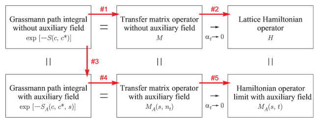
In this section we introduce a number of different lattice formulations using the example of zero-range attractive two-component fermions described by in Eq. (4). In Fig. (1) we show a schematic diagram of the different lattice formulations. The numbered arrows indicate the discussion order in the text.
Throughout our discussion of the lattice formalism we use dimensionless parameters and operators corresponding with physical values multiplied by the appropriate power of the spatial lattice spacing . In our notation the three-component integer vector labels the lattice sites of a three-dimensional periodic lattice with dimensions . The spatial lattice unit vectors are denoted , , . We use to label lattice steps in the temporal direction, and denotes the total number of lattice time steps. The temporal lattice spacing is given by , and is the ratio of the temporal to spatial lattice spacing. We also define , where is the fermion mass in lattice units.
III.1 Grassmann path integral without auxiliary field
For two-component fermions with zero-range attractive interactions we start with the lattice Grassmann path integral action without auxiliary fields. It is the simplest formulation in which to derive the lattice Feynman rules. Hence it is useful for both analytic lattice calculations and diagrammatic lattice Monte Carlo simulations Burovski et al. (2006a, b).
We let and be anticommuting Grassmann fields for spin . The Grassmann fields are periodic with respect to the spatial lengths of the lattice,
| (43) |
| (44) |
and antiperiodic along the temporal direction,
| (45) |
| (46) |
We write as shorthand for the integral measure,
| (47) |
We use the standard convention for Grassmann integration,
| (48) |
| (49) |
Local Grassmann densities are defined in terms of bilinear products of the Grassmann fields,
| (50) |
| (51) |
| (52) |
We consider the Grassmann path integral
| (53) |
where
| (54) |
The action consists of the free nonrelativistic fermion action
| (55) |
and a contact interaction between up and down spins. We consider the case where the coefficient is negative, corresponding with an attractive interaction. Since we are considering nonrelativistic lattice fermions with a quadratic dispersion relation, the lattice doubling problem associated with relativistic fermions does not occur.
In the grand canonical ensemble a common chemical potential is added for all spins. In this case the -dependent path integral is
| (56) |
where
| (57) |
and is the same as defined in Eq. (54), but with replaced by
III.2 Transfer matrix operator without auxiliary field
Let and denote fermion annihilation and creation operators satisfying the usual anticommutation relations
| (58) |
| (59) |
For any function we note the identity Creutz (2000)
| (60) |
where and are Grassmann variables. As before the symbols in Eq. (60) indicate normal ordering, and the trace is evaluated over all possible fermion states. This result can be checked explicitly using the complete set of possible functions .
It is useful to write Eq. (60) in a form that resembles a path integral over a short time interval with antiperiodic boundary conditions,
| (61) |
| (62) |
This result can be generalized to products of normal-ordered functions of several creation and annihilation operators. Let and denote fermion annihilation and creation operators for spin at lattice site . We can write any Grassmann path integral with instantaneous interactions as the trace of a product of operators using the identity Creutz (1988, 2000)
| (63) |
where .
Let us define the free nonrelativistic lattice Hamiltonian
| (64) |
as well as the lattice density operators
| (65) |
| (66) |
| (67) |
Using the correspondence Eq. (63), we can rewrite the path integral defined in Eq. (53) as a transfer matrix partition function,
| (68) |
where is the normal-ordered transfer matrix operator
| (69) |
Roughly speaking the transfer matrix operator is the exponential of the Hamiltonian operator over one Euclidean lattice time step, . In order to satisfy the identity Eq. (63), we work with normal-ordered transfer matrix operators. In the limit of zero temporal lattice spacing, , we obtain the Hamiltonian lattice formulation with Hamiltonian
| (70) |
This is also the defining Hamiltonian for the attractive Hubbard model in three dimensions.
In the grand canonical ensemble the effect of the chemical potential is equivalent to replacing by
| (71) |
For the Hamiltonian lattice formulation the effect of the chemical potential has the familiar form
| (72) |
III.3 Grassmann path integral with auxiliary field
We can re-express the Grassmann path integral using an auxiliary field coupled to the particle density. This lattice formulation has been used in several lattice studies at nonzero temperature Chen and Kaplan (2004); Lee and Schäfer (2005); Lee et al. (2004); Wingate (2005); Lee and Schäfer (2006a, b); Abe and Seki (2007a, b). Due to the simple contact interaction and the anticommutation of Grassmann variables, there is a large class of auxiliary-field transformations which reproduce the same action.
Let us write the Grassmann path integral using the auxiliary field
| (73) |
where
| (74) |
One possible example is a Gaussian-integral transformation similar to the original Hubbard-Stratonovich transformation Stratonovich (1958); Hubbard (1959) where
| (75) |
| (76) |
Another possibility is a discrete auxiliary-field transformation similar to that used in Ref. Hirsch (1983). In our notation this can be written as
| (77) |
| (78) |
where sgn equals for positive values and for negative values. In Ref. Lee (2008a) the performance of four different auxiliary-field transformations were compared.
We intentionally leave the forms for and unspecified, except for a number of conditions needed to recover Eq. (53) upon integrating out the auxiliary field . The first two conditions we set are
| (79) |
| (80) |
Since all even products of Grassmann variables commute, we can factor out the term in Eq. (73) involving the auxiliary field at . To shorten the notation we temporarily omit writing explicitly. We find
| (81) |
Therefore the last condition needed to recover Eq. (53) is
| (82) |
In the grand canonical ensemble, the auxiliary-field path integral at chemical potential is
| (83) |
where
| (84) |
III.4 Transfer matrix operator with auxiliary field
Using Eq. (63) and (73) we can write as a product of transfer matrix operators which depend on the auxiliary field,
| (85) |
where
| (86) |
This form has been used in a number of lattice simulations Müller et al. (2000); Bulgac et al. (2006); Lee (2006a, b, 2007a); Borasoy et al. (2007a); Juillet (2007); Abe and Seki (2007a, b); Borasoy et al. (2008a, b); Bulgac et al. (2008a); Lee (2008a); Bulgac et al. (2008b). In some of these studies the Hamiltonian limit is also taken.
In the grand canonical ensemble at chemical potential the partition function is
| (87) |
where is defined as
| (88) |
III.5 Improved lattice dispersion relations
In Ref. Bulgac et al. (2006, 2008a, 2008b) the transfer matrix operator at chemical potential was written as
| (89) |
in the Hamiltonian limit, with
| (90) |
This is different from in Eq. (71), but the two are the same in the Hamiltonian limit. The exponential interaction term in Eq. (89) was treated using a discrete auxiliary field. Also the matrix elements of were computed by Fast Fourier Transform in momentum space using the quadratic dispersion relation
| (91) |
with defined in the first Brillouin zone, . The motivation for this approach was to remove errors associated with the standard lattice dispersion relation
| (92) |
In Ref. Lee and Schäfer (2006a, b) lattice calculations at nonzero temperature and large scattering length found significant errors due to lattice artifacts. A detailed analysis in Ref. Lee and Thomson (2007) showed that the large errors were produced by broken Galilean invariance on the lattice. As an alternative to the momentum space approach in Eq. (91), improved lattice dispersions were investigated that could be derived from local lattice actions.
A class of improved single-particle dispersion relations can be defined on the lattice,
| (93) |
corresponds with the standard action, is the -improved action, and so on. The improved actions eliminate lattice artifacts in the Taylor expansion of about
| (94) |
The lattice action corresponding with contains hopping terms in each spatial direction that extend lattice steps beyond the nearest neighbor. The hopping coefficients for actions up to are shown in Table 1.
standard -improved -improved
In addition to these improved actions, new lattice actions called well-tempered actions were also introduced. These were defined implicitly in terms of their dispersion relation,
| (95) |
where the unknown constant was determined by the integral constraint,
| (96) |
At nonzero temperature and large scattering length the local well-tempered action corresponding with was shown to be comparable in accuracy to the nonlocal action defined by Lee and Thomson (2007).
IV Lattice formulations for low-energy nucleons
IV.1 Pionless effective field theory
Analogous with the continuum densities in Eq. (10), (11), (12), and (13), we define the lattice operators
| (97) |
| (98) |
| (99) |
| (100) |
At leading order in pionless effective field theory,
| (101) |
where
| (102) |
This formalism was used to study the triton and three-body forces on the lattice Borasoy et al. (2006). The triton can be regarded as an approximate example of the Efimov effect, which in the limit of zero range and infinite scattering length predicts a geometric sequence of trimer bound states Efimov (1971, 1993); Bedaque et al. (1999a, b); Bedaque et al. (2000); Braaten and Hammer (2006). The Efimov effect is not possible for two-component fermions due to Pauli exclusion but is allowed for more than two components. Once the binding energy of the trimer system is fixed, the binding energy of the four-body system is also determined Platter et al. (2004a); Platter et al. (2005); Hammer and Platter (2007). This is in analogy with the Tjon line relating the nuclear binding energies of 3H and 4He. In two dimensions a different geometric sequence has been predicted for zero-range attractive interactions. In this case the geometric sequence describes the binding energy of -body clusters as a function of in the large limit Hammer and Son (2004); Platter et al. (2004b); Blume (2005). These two-dimensional clusters have been studied using lattice effective field theory for up to particles and the geometric scaling has been confirmed Lee (2006b).
IV.2 Pionless effective field theory with auxiliary fields
In terms of auxiliary fields
| (103) |
where the auxiliary-field transfer matrix is
| (104) |
Let be the expectation value of the power of with respect to the measure
| (105) |
In order to reproduce the interactions in Eq. (102) we require that
| (106) |
The existence of a positive definite measure and real-valued is essential for Monte Carlo simulations without sign and phase oscillations. Sufficient and necessary conditions for the existence of a positive definite and real-valued is known in the mathematics literature as the truncated Hamburger moment problem. This problem has been solved Curto and Fialkow (1991); Adamyan et al. (2003); Chen et al. (2004), and the conditions are satisfied if and only if the block-Hankel matrix,
| (107) |
is positive semi-definite. The determinant of this matrix is . With an attractive two-nucleon force where the conditions are satisfied provided that the three-body interaction coefficient is not too large. We note that the positivity condition is spoiled more easily in the Hamiltonian limit where .
IV.3 Instantaneous free pion action
Before discussing lattice actions for chiral effective field theory, we first consider the lattice action for free pions with mass and purely instantaneous propagation,
| (108) |
The pion field is labelled with isospin index . Pion fields at different time steps and are not coupled due to the omission of time derivatives. This generates instantaneous propagation at each time step when computing one-pion exchange diagrams. It also eliminates unwanted pion couplings contributing to nucleon self-energy diagrams found in earlier work Lee et al. (2004). Though we call it a pion field, it is more accurate to regard as an auxiliary field which is used to reproduce the one-pion exchange potential on the lattice. If for example we wish to consider low-energy physical pions within the framework of chiral effective field theory Weinberg (1992), these scattering processes can be introduced perturbatively using external pion fields and additional auxiliary fields to reproduce the corresponding Feynman diagrams at each order.
Following the notation in Ref. Borasoy et al. (2007a), it is useful to define a rescaled pion field, ,
| (109) |
where
| (110) |
In terms of ,
| (111) |
and in momentum space we have
| (112) |
The instantaneous pion correlation function at spatial separation is
| (113) |
where
| (114) |
IV.4 Chiral effective field theory on the lattice
We define some lattice derivative notation which will be useful later. There are various ways to introduce spatial derivatives of the pion field on the lattice. The simplest definition for the gradient of is to define a forward-backward lattice derivative. For example we can write
| (115) |
This is the method used in Ref. Lee et al. (2004). One disadvantage is that it is a coarse derivative involving a separation distance of two lattice units. We can avoid this if we think of the pion lattice points as being shifted by lattice unit from the nucleon lattice points in each of the three spatial directions. For each nucleon lattice point we associate a pion lattice point ,
| (116) |
Then we have eight pion lattice points forming a cube centered at ,
| (117) |
For derivatives of the pion field we use the eight vertices of this unit cube on the lattice to define spatial derivatives. For each spatial direction and any lattice function we define
| (118) |
For double spatial derivatives of nucleon fields along direction we use the simpler definition,
| (119) |
At leading order in chiral effective field theory, the first partition function and transfer matrix operator considered in Ref. Borasoy et al. (2007a) was
| (120) |
where
| (121) |
and
| (122) |
This leading-order transfer matrix, labelled , has zero-range contact interactions analogous to the pionless transfer matrix in Eq. (102). The -improved action was used for .
A second leading-order partition function and transfer matrix was also considered,
| (123) |
where
| (124) |
The momentum-dependent coefficient function has the form
| (125) |
and the normalization factor is determined by the condition
| (126) |
The coefficient was determined by fitting to reproduce the correct average effective range for the two -wave channels. For small the function reduces to a Gaussian function,
| (127) |
This Gaussian smearing of the contact interactions in was found to remove four-nucleon clustering instabilities at lattice spacing MeV Borasoy et al. (2007a).
IV.5 Chiral effective field theory with auxiliary fields
Let us define the auxiliary-field action
| (128) |
In terms of auxiliary and pion fields, the partition function for LO1 is
| (129) |
where
| (130) |
and is the functional measure,
| (131) |
The instantaneous free pion action was already defined in Eq. (108).
For the LO2 action we have
| (132) |
The functional form of the transfer matrices are the same,
| (133) |
but for LO2 the auxiliary-field action has the non-local form
| (134) |
where the inverse function is defined as
| (135) |
IV.6 Next-to-leading-order interactions on the lattice
The lattice studies in Ref. Borasoy et al. (2008a, b) considered low-energy nucleon-nucleon scattering at momenta less than or equal to the pion mass, . On the lattice the ultraviolet cutoff momentum, , equals divided by the lattice spacing, . As noted earlier, serious numerical difficulties appear at large in Monte Carlo simulations of few- and many-nucleon systems. In attractive channels unphysical deeply-bound states appear at large . In other channels short-range repulsion becomes prominent, producing destructive sign or complex phase oscillations. The severity of the problem scales exponentially with system size and strength of the repulsive interaction.
In order to avoid these difficulties the approach advocated in Ref. Borasoy et al. (2008a, b) was to set the cutoff momentum as low as possible for describing physical momenta up to . In most of the published work so far the value chosen was MeV , corresponding with MeV. This coarse lattice approach is similar in motivation to the continuum low-momentum renormalization group approach using Bogner et al. (2003a, b).
For nearly all the two-pion exchange potential can be expanded in powers of
| (136) |
| (137) |
| (138) |
This expansion fails to converge only for near the cutoff scale , and so there is no practical advantage in keeping the full non-local structure of at this lattice spacing. Instead we simply use
| (139) |
| (140) |
where the terms in Eq. (138) with up to two powers of are absorbed in the definition of the coefficients for and .
Before describing the NLO lattice interactions in and , we first define lattice current densities for total nucleon number, spin, isospin, and spin-isospin. Similar to the definition of in Eq. (118), we use the eight vertices of a unit cube,
| (141) |
for . Let for be the reflection of the -component of about the center of the cube,
| (142) |
The -component of the SU(4)-invariant current density is defined as
| (143) |
Similarly for spin current density,
| (144) |
isospin current density,
| (145) |
and spin-isospin current density,
| (146) |
In Ref. Borasoy et al. (2008a) the next-to-leading-order transfer matrices and were defined by adding the following nine local interactions to the leading-order transfer matrices and . The two corrections to the leading-order contact interactions are
| (147) |
| (148) |
At next-to-leading order there are seven independent contact interactions with two derivatives. These are
| (149) |
| (150) |
| (151) |
| (152) |
| (153) |
| (154) |
| (155) |
IV.7 Model independence at fixed lattice spacing
In effective field theory calculations model independence is often tested by checking sensitivity on the cutoff scale . At a given order the difference between calculations for two different cutoff scales and should be no larger than the omitted corrections at the next order. On the lattice this test is problematic since the lattice spacing cannot be changed by a large amount due to computational constraints. Instead a different approach was introduced in Ref. Borasoy et al. (2008a) to test model independence at fixed lattice spacing which we summarize in the following.
The notation is used to denote two-nucleon operators with the following properties. is a sum of local two-nucleon interactions that is an analytic function of momenta below the cutoff scale and scales as or more powers of momenta in the asymptotic low-momentum limit. The term “quasi-local” is used to describe since the interactions are short-ranged. At fixed lattice spacing we may consider two different lowest-order actions with interactions of the form
| (156) | ||||
| (157) |
where and are different quasi-local operators with at least two powers of momenta. Since the leading-order interactions are iterated non-perturbatively the contact terms and in general have different coefficients. However low-energy physical observables should agree up to differences the same size as the omitted contributions at next-to-leading-order.
Similarly at next-to-leading order we may consider two different actions of the form
| (158) | ||||
| (159) |
where and are different quasi-local operators with at least four powers of momenta. Low-energy physical observables should again agree up to differences the same size as the omitted contributions at the next order.
This technique provides a method for testing model independence of the low-energy lattice effective theory without changing the lattice spacing. In principle however it is good to check model independence in multiple ways, including different variations for as well as changing the lattice spacing as much as allowed by computational constraints.
V Two-particle scattering on the lattice
V.1 Cubic rotation group
Lattice regularization reduces the SO rotational symmetry of continuous space to the cubic rotational group SO. This group is also known as the proper octahedral group and abbreviated as O. This lack of exact rotational symmetry complicates the extraction of partial wave amplitudes. SO consists of group elements generated by products of rotations about the , , axes. Since SO is discrete, angular momentum operators , , cannot be defined in the usual sense. Let be the group element for a rotation about the axis. The SO relation
| (160) |
can be used to define . The eigenvalues of are integers specified modulo 4. and may be defined in the same way using and .
There are five irreducible representations of the cubic rotational group. These are usually called , , , , and . Some of their properties and examples using low-order spherical harmonics are listed in Table 1. The elements of the total angular momentum representation of SO break up into smaller pieces associated with the five irreducible representations. Examples for are shown in Table 2 Johnson (1982).
Representation Example
V.2 Lüscher’s finite volume formula
Lüscher’s finite volume formula Lüscher (1986a, b, 1991) relates the energy levels of two-body states in a finite volume cubic box with periodic boundaries to the infinite volume scattering matrix. Recently Lüscher’s method has been studied and extended in a number of different ways. Several investigations have looked at asymmetric boxes Li and Liu (2004); Feng et al. (2004), while another considered small volumes where the lattice length is smaller than the scattering length Beane et al. (2004). There have also been studies of moving frames Rummukainen and Gottlieb (1995); Kim et al. (2005), Yukawa interactions de Soto and Carbonell (2006), pion-exchange windings around the periodic boundary Sato and Bedaque (2007), modifications at nonzero lattice spacing Seki and van Kolck (2006), and techniques to distinguish shallow bound states from scattering states using Levinson’s theorem Sasaki and Yamazaki (2006). Several recent studies derived finite volume formulas for systems of bosons with short-range interactions Beane et al. (2007b); Detmold and Savage (2008).
Lüscher’s method can be summarized as follows. We consider one up-spin and one down-spin in a periodic cube of length . The two-particle energy levels in the center-of-mass frame are related to the -wave phase shift,
| (161) |
where is the three-dimensional zeta function,
| (162) |
The -wave effective range expansion gives another expression for the left-hand side of Eq. (161),
| (163) |
In terms of , the energy of the two-particle scattering state is
| (164) |
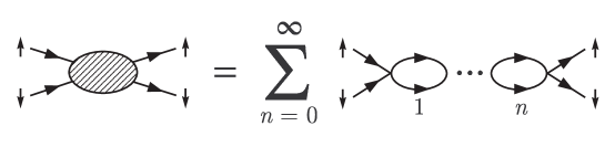
For the case of zero-range interactions, the location of the two-particle scattering pole is calculated by summing the bubble diagrams shown in Fig. 2.
The relation between and is Lee and Schäfer (2005)
| (165) |
where
| (166) |
for the standard lattice action. In this manner the coefficient can be tuned to produce the desired scattering length at infinite volume. Higher-order scattering parameters can also be extracted in this way. However for zero-range interactions the characteristic scale of these higher-order parameters is the lattice spacing, and so higher-order scattering corrections are the same size as lattice discretization errors produced by broken Galilean invariance and other lattice effects.
V.3 Spherical wall method
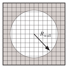
While Lüscher’s method is very useful at low momenta, it is not so useful for determining phase shifts on the lattice at higher energies and higher orbital angular momenta. Furthermore spin-orbit coupling and partial-wave mixing are difficult to measure accurately using Lüscher’s method due to multiple-scattering artifacts produced by the periodic cubic boundary. A more robust approach was proposed in Ref. Borasoy et al. (2007b) to measure phase shifts for nonrelativistic point particles on the lattice using a spherical wall boundary. Similar techniques have long been used in nuclear physics (see for example Problem 5-7 in Ref. Preston and Bhaduri (1975)) dating back to early work on -matrix methods Wigner and Eisenbud (1947). We summarize the method as follows.
A hard spherical wall boundary is imposed on the relative separation between the two particles at some chosen radius . This boundary condition removes copies of the interactions produced by the periodic lattice. Viewed in the center-of-mass frame we solve the Schrödinger equation for spherical standing waves which vanish at as indicated in Fig. 3.
When the combined intrinsic spin of the two interacting particles is zero there is no mixing between partial waves. At values of beyond the range of the interaction, the spherical standing wave can be decomposed as a superposition of products of spherical harmonics and spherical Bessel functions. Explicitly we have
| (167) |
where the center-of-mass energy of the spherical wave is
| (168) |
and the phase shift for partial wave is . We can determine from the energy of the standing wave, and the phase shift is calculated by setting the wavefunction in Eq. (167) equal to zero at the wall boundary,
| (169) |
| (170) |
On the lattice there is some ambiguity on the value of since the components of must be integer multiples of the lattice spacing. The ambiguity is resolved by fine-tuning the value of for each standing wave so that equals zero when the particles are non-interacting.
When the combined intrinsic spin of the two interacting particles is nonzero, spin-orbit coupling generates mixing between partial waves. For nucleons the interesting case is where there is mixing between and . We discuss this case here using the two-component notation,
| (171) |
for the radial part of the wavefunction. Since we are considering a two-channel system, there are two independent standing wave solutions of the form
| (172) |
at energy and
| (173) |
at . These can be used to derive the phase shifts and and mixing angle using Borasoy et al. (2007b)
| (174) |
| (175) |
| (176) |
| (177) |
The phase shifts and mixing angle in Eq. (174) and (176) are at momentum while the phase shifts and mixing angle in Eq. (175) and (177) are at momentum . Nearly equal pairs are used in solving the coupled constraints Eq. (174)-(177). In practice this amounts to considering the -radial excitation of together with the -radial excitation of . Then we use
| (178) |
| (179) |
| (180) |
for the phase shifts and mixing angle at , and
| (181) |
| (182) |
| (183) |
for the phase shifts and mixing angle at .
V.4 Scattering at NLO in chiral effective field theory
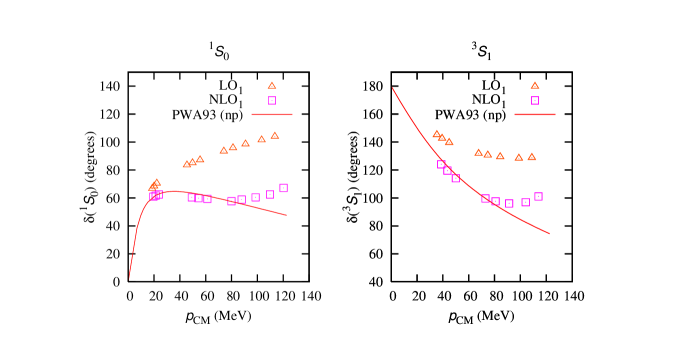
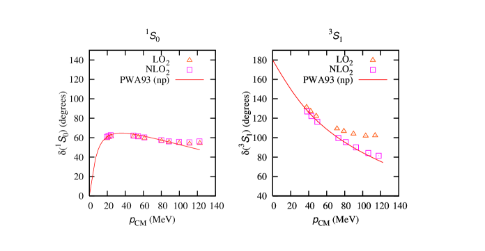
Lattice phase shifts and mixing angles at leading order and next-to-leading order were calculated in Ref. Borasoy et al. (2008a) using the spherical wall method at lattice spacings MeV, MeV. We summarize the results here. Fig. 4 shows energy levels for spin and isospin using lattice actions LO1 and LO2. The spherical wall is at radius lattice units where is a small positive number. The notation makes explicit that lattice units is inside the spherical wall but all lattice sites with lattice units lie outside. The solid lines indicate the exact energy levels which would reproduce data from the partial wave analysis in Stoks et al. (1993).
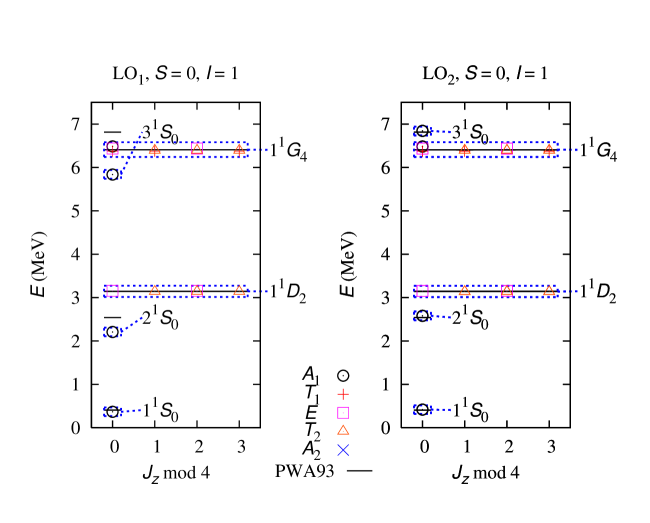
The energy levels for the standard action LO1 are to too low for the states, while the improved action LO2 is correct to a few of percent for all states. Deviations for higher partial waves are smaller than one percent for both LO1 and LO2.
The energy levels for spin , isospin , and lattice units are shown in Fig. 5.
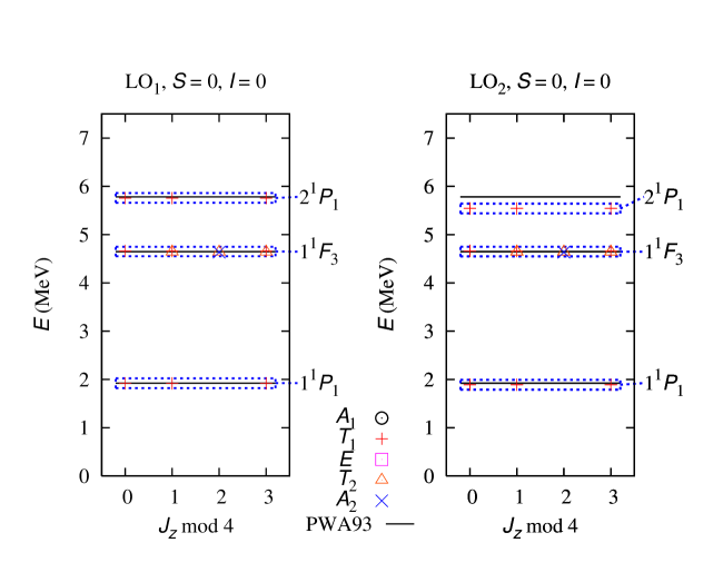
In this case LO1 is better for the states and is within one percent of the exact values. The LO2 energy levels are further away, though still within a few percent for the states.
In Ref. Borasoy et al. (2008a) the nine unknown operator coefficients at next-to-leading order were determined by matching three -wave scattering data points, four -wave scattering data points, as well as the deuteron binding energy and quadrupole moment. Each of the next-to-leading-order corrections were computed perturbatively. The -wave phase shifts for LO1 and NLO1 versus center-of-mass momentum are shown in Fig. 6, and the -wave phase shifts for LO2 and NLO2 are shown in Fig. 7. The NLO1 and NLO2 results are both in good agreement with partial wave results from Stoks et al. (1993). Systematic errors can be seen at momenta greater than about MeV and are larger for NLO1. But in both cases the deviations are at larger momenta and consistent with higher-order effects.
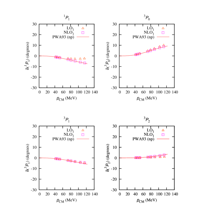
-wave phase shifts are shown in Fig. 8 and 9 Borasoy et al. (2008a). In this case the phase shifts are already close for LO1 and quite accurate for NLO1. This suggests that only a small correction is needed on top of -wave interactions produced by one-pion exchange. The results for LO2 and NLO2 are not quite as good. The Gaussian smearing introduced in LO2 produces attractive forces in each -wave channel that must be cancelled by next-to-leading-order corrections. However the residual deviations in the NLO2 results appear consistent with effects that can be cancelled by higher-order terms.
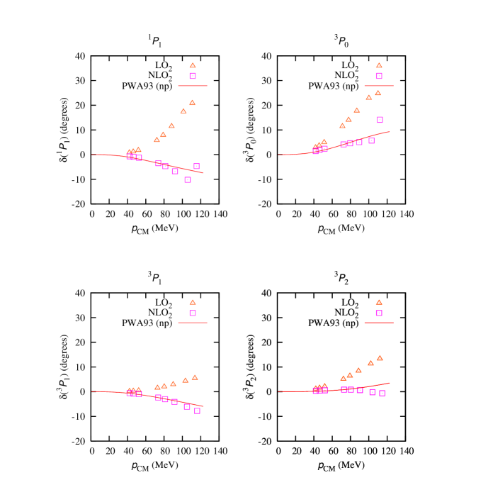
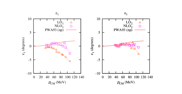
The mixing parameter for is shown in Fig. 10 Borasoy et al. (2008a). The mixing angle is defined according to the Stapp parameterization Stapp et al. (1957). Results for LO1 and NLO1 are on the left, and results for LO2 and NLO2 are on the right. The pairs of points connected by dotted lines indicate pairs of solutions at and for the coupled - channels. For LO1 we note that has the wrong sign. This suggests that the mixing angle may be more sensitive to lattice discretization errors than other scattering parameters. However for both NLO1 and NLO2 results the remaining deviations appear consistent with effects produced by higher-order interactions.
VI Monte Carlo algorithms
VI.1 Worldline methods
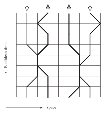
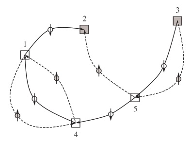
In bosonic systems or few-body systems where the problem of fermion sign cancellation is not severe, lattice simulations can be performed by directly sampling particle worldline configurations. We sketch an example of a lattice worldline configuration for two-component fermions in one spatial dimension in Fig. (11).
This technique was used in the simulation of the triton using pionless effective field theory Borasoy et al. (2006). A number of efficient cluster algorithms have been developed for condensed matter applications to generate new worldline configurations based on loop and worm updates Kawashima et al. (1994); Brower et al. (1998); Chandrasekharan and Wiese (1999); Evertz (2003); Kawashima and Harada (2004); Boninsegni et al. (2006).
While there are techniques which address the sign problem in certain cases Chandrasekharan and Wiese (1999), there is no general method known for eliminating sign oscillations in fermionic systems due to identical particle permutations. For Monte Carlo simulations extending over Euclidean time , the sign of the configuration, sgn, averaged over all configurations scales as
| (184) |
where is the physical ground state energy and is the fictitious ground state energy for bosons with the same interactions. The severity of the problem scales exponentially with the size of the system and inverse temperature. In nuclear physics the same issue arises in continuous-space worldline methods such as Green’s Function Monte Carlo and auxiliary-field diffusion Monte Carlo. In each case some supplementary condition is used to fix fermion nodal boundaries or constrain the domain of path integration Zhang et al. (1995, 1997).
VI.2 Determinantal diagrammatic methods
Determinantal diagrammatic Monte Carlo was used in Burovski et al. (2006a, b) to study two-component fermions in the unitarity limit near the critical point. This method is structurally similar to loop and worm updates of worldlines, however each configuration involves a complete summation of diagrams for a given set of vertices in Euclidean space. We discuss the method briefly here.
Let be the free-particle propagator in Euclidean space. We note that is real-valued. We define a set of vertex locations
| (185) |
where is the spatial location and is the Euclidean time for the vertex. We also define a matrix of vertex-to-vertex propagators , where
| (186) |
As an example we choose a set of five points , and in Fig. (12) we draw a Feynman diagram with vertices located at the coordinates of .
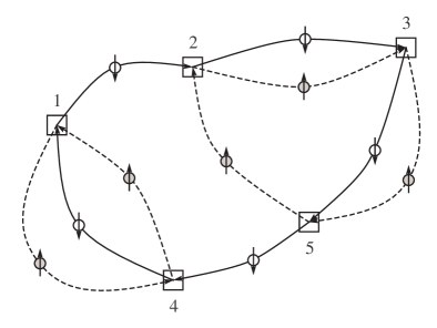
The propagators for the down spins in Fig. (12) give one term in the expansion of ,
| (187) |
The same is true for the up spins in Fig. (12),
| (188) |
and the determinant expansion shows that there is a relative minus sign between the up and down contributions. From this example it is clear that the total contribution of all Feynman diagrams with vertices given by is
| (189) |
We note that is positive definite when the interaction is attractive, . Convergence of the series in powers of is guaranteed by finiteness of the Grassmann path integral at finite volume.
In order to compute the full path integral
| (190) |
the sampling of vertex configurations can be generated using a worm algorithm that produces closed loop diagrams such as Fig. (12) as well as single worm diagrams such as the example shown in Fig. (13). In this diagram pairs of fermion lines are created at vertex and annihilated at vertex . The sum of all diagrams of the type shown in Fig. (13) can be written in terms of the derivative of with respect to ,
| (191) |
From this we see that the contribution from worm diagrams is also positive. These diagrams are used to calculate the expectation value of the pair correlation function,
| (192) |
Further details of the worm updating algorithm and determinantal diagrammatic Monte Carlo can be found in Burovski et al. (2006a, b); Van Houcke et al. (2008).
VI.3 Projection Monte Carlo with auxiliary field
Projection Monte Carlo was used to compute the ground state energy of two-components fermions at unitarity Lee (2006a, 2007a); Juillet (2007); Lee (2008a). It was also used to study light nuclei and dilute neutrons in chiral effective field theory Borasoy et al. (2007a, 2008b). We briefly describe the method here using first the example of zero-range attractive two-component fermions.
Let be the ground state for the interacting system of up spins and down spins. Let be the normalized Slater-determinant ground state for a non-interacting system of up spins and down spins. We use the auxiliary-field transfer matrix defined in Eq. (86) to construct the Euclidean-time projection amplitude
| (193) |
where . We define as the transient energy measured at time ,
| (194) |
So long as the overlap between and the ground state of the interacting system is nonzero, the ground state is given by the limit
| (195) |
As a result of normal ordering, consists of single-particle operators interacting with the background auxiliary field and contains no direct interactions between particles. Therefore we can write
| (196) |
where
| (197) |
for matrix indices . are single-particle momentum states comprising the Slater-determinant state . The single-particle interactions in are the same for both up and down spins. Since the matrix is real-valued, the square of the determinant is nonnegative and there is no problem with sign oscillations. New configurations are accepted or rejected according to the probability weight
| (198) |
We note that is only an matrix. This is considerably smaller than matrices encountered in most other determinantal methods and contributes to the relative efficiency of projection Monte Carlo. For the case when the auxiliary field is continuous, new configurations can be generated using a non-local updating algorithm called hybrid Monte Carlo Scalettar et al. (1986); Gottlieb et al. (1987); Duane et al. (1987). This scheme is widely used in lattice QCD simulations.
VI.4 Hybrid Monte Carlo
We describe the hybrid Monte Carlo algorithm in general terms for probability weight
| (199) |
which depends on the lattice field and some function which may be a non-local function of . The method proposes new configurations by means of molecular dynamics trajectories for
| (200) |
where is the conjugate momentum for . The steps of the algorithm are as follows.
-
Step 1:
Select an arbitrary initial configuration .
-
Step 2:
Select a configuration according to the Gaussian random distribution
(201) -
Step 3:
For each let
(202) for some small positive .
-
Step 4:
For steps , let
(203) (204) for each
-
Step 5:
For each let
(205) -
Step 6:
Select a random number If
(206) then set . Otherwise leave as is. In either case go back to Step 2 to start a new trajectory.
VI.5 Grand canonical simulations with auxiliary field
In Eq. (87) we introduced the partition function for zero-range attractive two-component fermions at chemical potential ,
| (207) |
with auxiliary-field transfer matrix
| (208) |
Let be the quantum state with one particle at lattice site and no other particles. As in Eq. (197), we define the one-particle matrix amplitudes
| (209) |
However in this case the matrix has dimensions .
The trace over states in Eq. (207) can now be written as
| (210) |
New configurations for can be updated locally using the Metropolis algorithm. This method has been used in lattice calculations to study the thermodynamics of two-component fermions near unitarity Abe and Seki (2007a, b); Bulgac et al. (2006, 2008a, 2008b) and, more generally, the attractive Hubbard model and repulsive Hubbard model near half-filling in various spatial dimensions Sewer et al. (2002); Hirsch (1983). A review of numerical aspects of this method can be found in Loh and Gubernatis (1992).
VI.6 Pseudofermion methods
The same grand canonical partition function in Eq. (207) can be evaluated in the Grassmann path integral formulation with auxiliary fields,
| (211) |
where
| (212) |
and
| (213) |
We note that is a bilinear form coupling and with a block-diagonal spin structure which is the same for up and down spins,
| (214) |
Therefore the integration over Grassmann variables gives the square of the determinant of ,
| (215) |
This result can also be written as a path integral over a complex bosonic field ,
| (216) |
where
| (217) |
The bosonic field is called a pseudofermion field. This technique was first implemented for fermions in lattice QCD Weingarten and Petcher (1981). The non-local action in Eq. (217) can be updated using a non-local algorithm such as hybrid Monte Carlo. Typically an iterative sparse matrix solver is used such as the conjugate gradient method.
Pseudofermion methods have been used to study the thermodynamics of two-component fermions near unitarity Lee and Schäfer (2005); Wingate (2005); Lee and Schäfer (2006a, b); Abe and Seki (2007a, b). For the case when an external field is coupled to the difermion pair,
| (218) |
the block structure of the Grassmann action is more complicated. However the analysis in Ref. Chen and Kaplan (2004) shows that the path integral can still be written in terms of a positive-definite Pfaffian. Lattice simulations using this formalism were carried out using pseudofermion methods and hybrid Monte Carlo Wingate (2005).
VI.7 Applications to low-energy nucleons
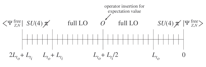
The projection Monte Carlo method with auxiliary fields has been used to study low-energy nucleons in chiral effective field theory Borasoy et al. (2007a, 2008a, 2008b). A two-step approach was used where a pionless SU(4)-symmetric transfer matrix acts as an approximate and inexpensive low-energy filter at the beginning and end time steps. For time steps in the midsection, the full leading-order transfer matrix was used and next-to-leading-order operators were evaluated perturbatively by insertion at the middle time step. A schematic overview of the transfer matrix calculation is shown in Fig. 14.
The pionless SU(4)-symmetric transfer matrix is computationally inexpensive because the path integral in the SU(4) limit is strictly positive for any even number of nucleons with either spin-singlet or isospin-singlet quantum numbers Chen et al. (2004). Although there is no positivity theorem for odd numbers of nucleons, sign oscillations are relatively mild in odd systems which are only one particle or one hole away from an even system with no sign oscillations. Some general results on positivity of the path integral and spectral inequalities in pionless effective theory have been discussed in Lee (2004, 2005); Chen et al. (2004); Wu and Zhang (2005).
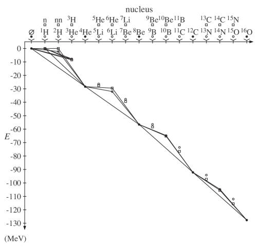
SU(4) symmetry arises naturally in the limit of large number of colors Kaplan and Savage (1996); Kaplan and Manohar (1997), and the fact that both the spin-singlet and spin-triplet nucleon scattering lengths are unusually large suggests that the physics of low-energy nucleons is close to the Wigner limit Mehen et al. (1999); Epelbaum et al. (2002b). In Ref. Lee (2007b) a general theorem on path integral positivity was derived for interactions governed by an SU-invariant two-body potential whose Fourier transform is negative definite. It was also shown that as a consequence of the path integral positivity, the particle spectrum must satisfy a number of convexity lower bounds with respect to particle number. In Fig. (15) we draw all SU(4) convexity bounds applied to the spectrum of light nuclei with up to nucleons Lee (2007b). We note that each of the lower bound constraints are satisfied. While these results do not imply that Monte Carlo simulations of nucleons using chiral effective theory can be performed without sign or phase oscillations, they do suggest that the simulations are possible with only relatively mild cancellations given the approximate SU(4) symmetry and attractive interactions at low-energies.
VII Some recent results
VII.1 Ground state energy at unitarity
At zero temperature there are no dimensionful parameters in the unitarity limit other than particle density. For up spins and down spins in a given volume we denote the energy of the unitarity-limit ground state as . For the same volume we call the energy of the free non-interacting ground state and define the dimensionless ratio
| (219) |
The parameter is defined as the thermodynamic limit for the spin-unpolarized system,
| (220) |
Several experiments have measured using density profiles of 6Li and 40K expanding upon release from a harmonic trap. Some recent measured values for are Kinast et al. (2005), Stewart et al. (2006), and Bartenstein et al. (2004). There is some disagreement among these recent measurements as well as with larger values for were reported in earlier experiments O’Hara et al. (2002); Bourdel et al. (2003); Gehm et al. (2003).
There are a number of analytic calculations for using techniques such as BCS saddle point and variational approximations, Padé approximations, mean field theory, density functional theory, exact renormalization group, dimensional -expansions, and large- expansions Engelbrecht et al. (1997); Baker (1999); Heiselberg (2001); Perali et al. (2004a); Schäfer et al. (2005); Papenbrock (2005); Nishida and Son (2006, 2007); Chen (2007); Krippa (2007); Arnold et al. (2007); Nikolic and Sachdev (2007); Veillette et al. (2007). The values for range from to . Fixed-node Green’s function Monte Carlo simulations for a periodic cube find to be for Carlson et al. (2003a) and for larger Astrakharchik et al. (2004); Carlson and Reddy (2005). A restricted path integral Monte Carlo calculation finds similar results Akkineni et al. (2006), and a mean-field projection lattice calculation yields Juillet (2007).
There have also been simulations of two-component fermions on the lattice in the unitarity limit at nonzero temperature. When data are extrapolated to zero temperature the results of Bulgac et al. (2006, 2008a) produce a value for similar to the fixed-node results. The same is true for Burovski et al. (2006a, b), though with significant error bars. The extrapolated zero temperature lattice results from Lee and Schäfer (2006a, b) established a bound, .
Recent lattice calculations in the grand canonical ensemble yield a value for Abe and Seki (2007a, b). These calculations used lattice volumes of , , , and also probed the behavior at finite scattering length. In Fig. (16) we show as a function of Abe and Seki (2007b). The circles show the lattice results of Abe and Seki (2007b), and the dotted line shows a quadratic fit through the points. The squares are fixed-node Green’s function Monte Carlo results Astrakharchik et al. (2004), and the solid line corresponds with results calculated using the epsilon expansion Chen and Nakano (2007).

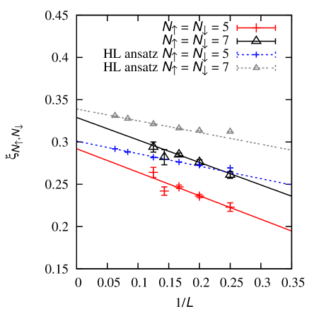
In Ref. Lee (2006a) was calculated on the lattice using Euclidean time projection in small volumes where it was estimated that . More recent results using a technique called the symmetric heavy-light ansatz found similar values for at the same lattice volumes and estimated in the continuum and thermodynamic limits Lee (2008b). A very recent lattice calculation using Euclidean time projection with a bounded continuous auxiliary field used lattice volumes , , , , and extrapolated to the continuum limit Lee (2008a). The results found were
| (221) |
| (222) |
In Fig. 17 we show results for and at finite and the corresponding continuum limit extrapolations Lee (2008a). For comparison we also show Hamiltonian lattice results using the symmetric heavy-light ansatz in the lowest filling approximation Lee (2008b). These lattice calculations show close agreement with each other and disagreement with fixed-node Green’s function Monte Carlo results for the same number of particles in a periodic cube Carlson et al. (2003a).
VII.2 Critical temperature at unitarity
At unitarity the critical temperature can be written as a fraction of the Fermi energy. Experimentally has been measured using trapped 6Li and found to be Kinast et al. (2005). However the interpretation of this result is made difficult by modifications caused by the trap potential and the problem of relating empirical and actual temperature scales Perali et al. (2004b); Bulgac (2005); Burovski et al. (2006a). A number of approximate theoretical calculations suggest a value for the critical temperature above Nozieres and Schmitt-Rink (1985); Holland et al. (2001); Perali et al. (2004b) as well as below Haussmann (1994); Ohashi and Griffin (2002); Liu and Hu (2005) the Bose-Einstein condensation temperature . An epsilon expansion calculation around yields while the epsilon expansion around yields Nishida and Son (2006, 2007); Nishida (2007). Omitting terms at , the large expansion yields Nikolic and Sachdev (2007). A continuum-space restricted path integral Monte Carlo calculation found Akkineni et al. (2006).
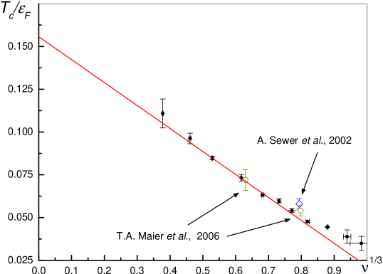
Lattice simulations measuring long-range order in the pair correlation function find values Lee and Schäfer (2006b), Bulgac et al. (2008b), Burovski et al. (2006a, b), and Abe and Seki (2007b). The spread in values can likely be explained by lattice discretization errors, which are visible in Fig. (18) showing the dependence of on , where is the lattice filling fraction Burovski et al. (2006a, b). The simulations were done with lattice sizes , , . The point labelled A. Sewer et al. corresponds with Sewer et al. (2002), while the points labelled T. A. Maier et al. correspond with unpublished work which appears to be unavailable in print. The results of Wingate (2005) are also consistent with a point along this line.
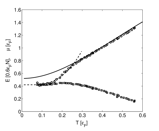
While coherence measurements of the pair correlation function in Bulgac et al. (2008b) indicate an upper bound on the critical temperature, , the calculation of the average energy has a peculiar structure at at lattice volumes , Bulgac et al. (2006, 2008b). This data is shown in Fig. (19). The physical significance of this effect is presently unknown. Meanwhile lattice calculations of the pair correlation function using projection Monte Carlo find low-energy string-like excitations winding around the periodic lattice Lee (2007a). These excitations may play some role in spoiling pair coherence at relatively low temperatures.
VII.3 Dilute neutron matter at NLO in chiral effective field theory
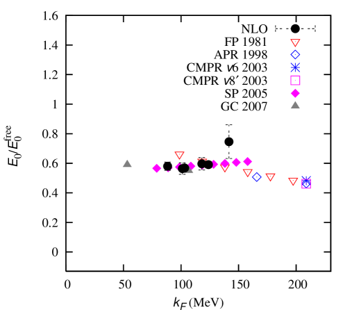
In Ref. Borasoy et al. (2008b) the ground state energy of dilute neutrons was calculated on the lattice at next-to-leading order in chiral effective field theory. The simulations used and neutrons in lattice volumes , , at lattice spacings MeV, MeV. In Fig. 20 we show results for the ratio of the interacting ground state energy to non-interacting ground state energy, , as a function of Fermi momentum . For comparison we show other results from the literature: FP 1981 Friedman and Pandharipande (1981), APR 1998 Akmal et al. (1998), CMPR and Carlson et al. (2003b), SP 2005 Schwenk and Pethick (2005), and GC 2007 Gezerlis and Carlson (2008). There is good agreement between the different results near MeV, but there is some disagreement on the slope.
The analysis in Ref. Borasoy et al. (2008b) shows that much of the -wave contributions from different spin channels cancel numerically.
VII.4 Comparison with other methods and future outlook
At nonzero temperature there are unfortunately very few ab initio calculations that can be used to compare with results obtained using lattice effective field theory. We have already mentioned a restricted path integral Monte Carlo calculation for cold atoms at unitarity Akkineni et al. (2006). However the size of systematic errors due to path restriction is difficult to estimate, and the final result for the critical temperature is in strong disagreement with each of the lattice results presented above.
More comparisons can be made for calculations of low energy spectra. At present the most accurate ab initio calculations of light nuclei binding energies for up to twelve nucleons have been obtained using Green’s Function Monte Carlo. The overall accuracy of these calculations are at the level. Current lattice calculations are not as accurate as this, but it is hoped that lattice simulations for light nuclei at N3LO in the future can reach comparable accuracies. At cutoff momentum MeV, No-Core Shell Model calculations using the NNLO chiral potential (plus N3LO terms for the two-nucleon potential) give binding energies for 6Li and 7Li at accuracy Nogga et al. (2006); Nogga (2006). The first lattice effective field theory calculations at NNLO are currently in progress. Preliminary results for lattice spacing MeV give an alpha binding energy accurate at the level Epelbaum et al. . However much further work remains in developing the lattice formalism at higher order and studying larger nuclei.
For the ground state of cold atoms at unitarity and dilute neutron matter, the quality of lattice effective field theory calculations are competitive with or exceed other computational approaches. Here the relative success of lattice simulations over other methods is probably due to the nature of the ground state and the use of determinantal Monte Carlo. For cold atoms at unitarity and dilute neutron matter the competition between attractive binding forces and Fermi antisymmetry is somewhat evenly matched, resulting in a complicated superfluid ground state somewhere in between BCS and BEC. This makes it difficult to use techniques where nodal constraints must be approximately guessed and easier to rely on determinantal Monte Carlo methods which automatically incorporate Fermi antisymmetry.
In addition to probing more nucleons and higher orders in effective field theory, future work must also probe simulations at larger lattice volumes. This includes both smaller physical lattice spacings as well as larger physical volumes. The transition from small lattice systems to large production runs should be possible as more experience and data is collected on the efficiency of various lattice algorithms and more computing resources are devoted to important calculations. It is probably unlikely that lattice effective field theory simulations can match the spatial lattice lengths used in some large-scale lattice QCD simulations. For cold atom simulations at unitarity the most significant computational barrier with increasing system size is the increase in condition number for the auxiliary field matrices . Similar computational slowdown occurs in unquenched lattice QCD simulations at very small sea quark masses or at large chemical potential (in addition to the problem caused by complex phase oscillations).
For a single bound nucleus it is not necessary to probe volumes much larger than the size of the bound state since the finite volume errors are exponentially small. In this case it would be more useful to probe smaller physical lattice spacings, as much as constraints such as sign or complex phase oscillations will allow. For unbound nuclear systems the finite volume dependence of energy levels should be more interesting. This data can be used to probe nucleon-nucleus scattering or nucleus-nucleus scattering using Lüscher’s finite volume scattering method.
It is difficult to predict the development of the field in the future, but one general hope is that collaborative efforts develop with researchers not directly involved in large-scale lattice calculations. One working model has already been pioneered in the lattice QCD community, where large numbers of gauge configurations are stored and shared for general use. A similar model may be useful for lattice effective field theory calculations for systems with significant general interest.
VIII Summary
In this article we have reviewed the current literature on lattice simulations for few- and many-body systems. We discussed methods which combine the theoretical framework of effective field theory with computational lattice methods. The lattice spacing serves as the ultraviolet cutoff for the low-energy effective theory, and all interactions are included up to some chosen order in power counting. By increasing the order, the accuracy at low energies can be systematically improved. One feature of this approach is the ability to study several different phenomena using exactly the same lattice action. Another feature of the lattice effective field theory approach is the close theoretical link with standard analytic tools used in effective field theory calculations. The approach also benefits from the computational flexibility provided by a number of efficient lattice algorithms. We have discussed many of these in this article.
The idea of lattice simulations using effective field theory is relatively new, and this review article represents a snapshot of the current progress in the field. We have attempted to cover the relevant principles from effective field theory as well as different formalisms and algorithms used in recent lattice calculations. We have focused much attention on techniques which can be applied to both cold atoms and low-energy nuclear physics as well as common methods used in work by different collaborations.
Acknowledgements
The author thanks a long list of collaborators and colleagues for discussing work and topics covered in this review. The list includes Bugra Borasoy, Aurel Bulgac, Shailesh Chandrasekharan, Jiunn-Wei Chen, Evgeny Epelbaum, Hans Hammer, Hermann Krebs, Ulf-G. Meißner, Nikolay Prokof’ev, Gautam Rupak, Thomas Schäfer, Ryoichi Seki, Boris Svistunov, Bira van Kolck, and Matt Wingate. This work is supported in part by DOE grant DE-FG02-03ER41260.
References
- Hammond et al. (1994) B. L. Hammond, J. W. A. Lester, and P. J. Reynolds, Monte Carlo Methods in Ab Initio Quantum Chemistry (World Scientific, Singapore, 1994).
- Foulkes et al. (2001) W. M. C. Foulkes, L. Mitas, R. J. Needs, and G. Rajagopal, Rev. Mod. Phys. 73, 33 (2001).
- Ceperley (1995) D. M. Ceperley, Rev. Mod. Phys. 67, 279 (1995).
- Carlson and Schiavilla (1998) J. Carlson and R. Schiavilla, Rev. Mod. Phys. 70, 743 (1998).
- von der Linden (1992) W. von der Linden, Phys. Rep. 220, 53 (1992).
- Muroya et al. (2003) S. Muroya, A. Nakamura, C. Nonaka, and T. Takaishi, Prog. Theor. Phys. 110, 615 (2003), eprint hep-lat/0306031.
- Davies (2002) C. Davies (2002), eprint hep-ph/0205181.
- Kuramashi et al. (1993) Y. Kuramashi, M. Fukugita, H. Mino, M. Okawa, and A. Ukawa, Phys. Rev. Lett. 71, 2387 (1993).
- Aoki et al. (2003) S. Aoki et al. (CP-PACS), Phys. Rev. D67, 014502 (2003), eprint hep-lat/0209124.
- Lin et al. (2003) C. J. D. Lin, G. Martinelli, E. Pallante, C. T. Sachrajda, and G. Villadoro, Phys. Lett. B553, 229 (2003), eprint hep-lat/0211043.
- Beane et al. (2006a) S. R. Beane, P. F. Bedaque, K. Orginos, and M. J. Savage (NPLQCD), Phys. Rev. D73, 054503 (2006a), eprint hep-lat/0506013.
- Beane et al. (2006b) S. R. Beane et al., Phys. Rev. D74, 114503 (2006b), eprint hep-lat/0607036.
- Beane et al. (2008a) S. R. Beane et al. (NPLQCD), Phys. Rev. D77, 094507 (2008a), eprint 0709.1169.
- Fukugita et al. (1995) M. Fukugita, Y. Kuramashi, M. Okawa, H. Mino, and A. Ukawa, Phys. Rev. D52, 3003 (1995), eprint hep-lat/9501024.
- Beane et al. (2004) S. R. Beane, P. F. Bedaque, A. Parreno, and M. J. Savage, Phys. Lett. B585, 106 (2004), eprint hep-lat/0312004.
- Beane et al. (2007a) S. R. Beane et al. (NPLQCD), Nucl. Phys. A794, 62 (2007a), eprint hep-lat/0612026.
- Beane et al. (2006c) S. R. Beane, P. F. Bedaque, K. Orginos, and M. J. Savage, Phys. Rev. Lett. 97, 012001 (2006c), eprint hep-lat/0602010.
- Ishii et al. (2007) N. Ishii, S. Aoki, and T. Hatsuda, Phys. Rev. Lett. 99, 022001 (2007), eprint nucl-th/0611096.
- Aoki et al. (2008) S. Aoki, T. Hatsuda, and N. Ishii (2008), eprint 0805.2462.
- Nemura et al. (2008) H. Nemura, N. Ishii, S. Aoki, and T. Hatsuda (2008), eprint 0806.1094.
- Beane et al. (2008b) S. R. Beane, K. Orginos, and M. J. Savage (2008b), eprint 0805.4629.
- Nogga et al. (2000) A. Nogga, H. Kamada, and W. Gloeckle, Phys. Rev. Lett. 85, 944 (2000), eprint nucl-th/0004023.
- Stoks et al. (1994) V. G. J. Stoks, R. A. M. Klomp, C. P. F. Terheggen, and J. J. de Swart, Phys. Rev. C49, 2950 (1994), eprint nucl-th/9406039.
- Machleidt et al. (1996) R. Machleidt, F. Sammarruca, and Y. Song, Phys. Rev. C53, 1483 (1996), eprint nucl-th/9510023.
- Wiringa et al. (1995) R. B. Wiringa, V. G. J. Stoks, and R. Schiavilla, Phys. Rev. C51, 38 (1995), eprint nucl-th/9408016.
- Coon and Gloeckle (1981) S. A. Coon and W. Gloeckle, Phys. Rev. C23, 1790 (1981).
- Pudliner et al. (1997) B. S. Pudliner, V. R. Pandharipande, J. Carlson, S. C. Pieper, and R. B. Wiringa, Phys. Rev. C56, 1720 (1997), eprint nucl-th/9705009.
- Epelbaum et al. (2001) E. Epelbaum et al., Phys. Rev. Lett. 86, 4787 (2001), eprint nucl-th/0007057.
- Nogga et al. (2004) A. Nogga, S. K. Bogner, and A. Schwenk, Phys. Rev. C70, 061002 (2004), eprint nucl-th/0405016.
- Bogner et al. (2003a) S. K. Bogner, T. T. S. Kuo, A. Schwenk, D. R. Entem, and R. Machleidt, Phys. Lett. B576, 265 (2003a), eprint nucl-th/0108041.
- Bogner et al. (2003b) S. K. Bogner, T. T. S. Kuo, and A. Schwenk, Phys. Rept. 386, 1 (2003b), eprint nucl-th/0305035.
- Wiringa et al. (2000) R. B. Wiringa, S. C. Pieper, J. Carlson, and V. R. Pandharipande, Phys. Rev. C62, 014001 (2000), eprint nucl-th/0002022.
- Pieper and Wiringa (2001) S. C. Pieper and R. B. Wiringa, Ann. Rev. Nucl. Part. Sci. 51, 53 (2001), eprint nucl-th/0103005.
- Pieper et al. (2001) S. C. Pieper, V. R. Pandharipande, R. B. Wiringa, and J. Carlson, Phys. Rev. C64, 014001 (2001), eprint nucl-th/0102004.
- Pieper et al. (2002) S. C. Pieper, K. Varga, and R. B. Wiringa, Phys. Rev. C66, 044310 (2002), eprint nucl-th/0206061.
- Wiringa and Pieper (2002) R. B. Wiringa and S. C. Pieper, Phys. Rev. Lett. 89, 182501 (2002), eprint nucl-th/0207050.
- Pieper et al. (2004) S. C. Pieper, R. B. Wiringa, and J. Carlson, Phys. Rev. C70, 054325 (2004), eprint nucl-th/0409012.
- Nollett et al. (2007) K. M. Nollett, S. C. Pieper, R. B. Wiringa, J. Carlson, and G. M. Hale, Phys. Rev. Lett. 99, 022502 (2007), eprint nucl-th/0612035.
- Gezerlis and Carlson (2008) A. Gezerlis and J. Carlson, Phys. Rev. C77, 032801 (2008), eprint 0711.3006.
- Pieper (2007) S. C. Pieper (2007), eprint 0711.1500.
- Fantoni et al. (2001) S. Fantoni, A. Sarsa, and K. E. Schmidt, Phys. Rev. Lett. 87, 181101 (2001), eprint nucl-th/0106026.
- Sarsa et al. (2003) A. Sarsa, S. Fantoni, K. E. Schmidt, and F. Pederiva, Phys. Rev. C68, 024308 (2003), eprint nucl-th/0303035.
- Pederiva et al. (2004) F. Pederiva, A. Sarsa, K. E. Schmidt, and S. Fantoni, Nucl. Phys. A742, 255 (2004), eprint nucl-th/0403069.
- Chang et al. (2004) S. Y. Chang et al., Nucl. Phys. A746, 215 (2004), eprint nucl-th/0401016.
- Gandolfi et al. (2007) S. Gandolfi, F. Pederiva, S. Fantoni, and K. E. Schmidt, Phys. Rev. Lett. 99, 022507 (2007), eprint arXiv:0704.1774 [nucl-th].
- Gandolfi et al. (2008) S. Gandolfi, A. Y. Illarionov, S. Fantoni, F. Pederiva, and K. E. Schmidt (2008), eprint 0805.2513.
- Navratil et al. (2000) P. Navratil, J. P. Vary, and B. R. Barrett, Phys. Rev. Lett. 84, 5728 (2000), eprint nucl-th/0004058.
- Fayache et al. (2001) M. S. Fayache, J. P. Vary, B. R. Barrett, P. Navratil, and S. Aroua (2001), eprint nucl-th/0112066.
- Navratil and Ormand (2003) P. Navratil and W. E. Ormand, Phys. Rev. C68, 034305 (2003), eprint nucl-th/0305090.
- Caurier and Navratil (2006) E. Caurier and P. Navratil, Phys. Rev. C73, 021302 (2006), eprint nucl-th/0512015.
- Forssen et al. (2005) C. Forssen, P. Navratil, W. E. Ormand, and E. Caurier, Phys. Rev. C71, 044312 (2005), eprint nucl-th/0412049.
- Nogga et al. (2006) A. Nogga, P. Navratil, B. R. Barrett, and J. P. Vary, Phys. Rev. C73, 064002 (2006), eprint nucl-th/0511082.
- Navratil et al. (2007) P. Navratil, V. G. Gueorguiev, J. P. Vary, W. E. Ormand, and A. Nogga, Phys. Rev. Lett. 99, 042501 (2007), eprint nucl-th/0701038.
- Stetcu et al. (2006) I. Stetcu, B. R. Barrett, and U. van Kolck (2006), eprint nucl-th/0609023.
- Kamada et al. (2001) H. Kamada et al., Phys. Rev. C64, 044001 (2001), eprint nucl-th/0104057.
- Brockmann and Frank (1992) R. Brockmann and J. Frank, Phys. Rev. Lett. 68, 1830 (1992).
- Walecka (1974) J. D. Walecka, Annals Phys. 83, 491 (1974).
- Müller et al. (2000) H. M. Müller, S. E. Koonin, R. Seki, and U. van Kolck, Phys. Rev. C61, 044320 (2000), eprint nucl-th/9910038.
- Sewer et al. (2002) A. Sewer, X. Zotos, and H. Beck, Phys. Rev. B66, 140504(R) (2002), eprint cond-mat/0204053.
- Chen and Kaplan (2004) J.-W. Chen and D. B. Kaplan, Phys. Rev. Lett. 92, 257002 (2004), eprint hep-lat/0308016.
- Chandrasekharan et al. (2004) S. Chandrasekharan, M. Pepe, F. D. Steffen, and U. J. Wiese, Nucl. Phys. Proc. Suppl. 129, 507 (2004), eprint hep-lat/0309093.
- Shushpanov and Smilga (1999) I. A. Shushpanov and A. V. Smilga, Phys. Rev. D59, 054013 (1999), eprint hep-ph/9807237.
- Lewis and Ouimet (2001) R. Lewis and P.-P. A. Ouimet, Phys. Rev. D64, 034005 (2001), eprint hep-ph/0010043.
- Borasoy et al. (2003) B. Borasoy, R. Lewis, and P.-P. A. Ouimet (2003), eprint hep-lat/0310054.
- Lee et al. (2004) D. Lee, B. Borasoy, and T. Schäfer, Phys. Rev. C70, 014007 (2004), eprint nucl-th/0402072.
- Furnstahl et al. (2008) R. J. Furnstahl, G. Rupak, and T. Schafer (2008), eprint arXiv:0801.0729 [nucl-th].
- Bethe (1949) H. A. Bethe, Phys. Rev. 76, 38 (1949).
- Braaten and Hammer (2006) E. Braaten and H.-W. Hammer, Phys. Rept. 428, 259 (2006).
- Eagles (1969) D. M. Eagles, Phys. Rev. 186, 456 (1969).
- Leggett (1980) A. J. Leggett, in Modern Trends in the Theory of Condensed Matter. Proceedings of the XVIth Karpacz Winter School of Theoretical Physics, Karpacz, Poland, 1980 (Springer-Verlag, Berlin, 1980), p. 13.
- Nozieres and Schmitt-Rink (1985) P. Nozieres and S. Schmitt-Rink, J. Low Temp. Phys. 59, 195 (1985).
- Chen et al. (2005) Q. Chen, J. Stajic, S. Tan, and K. Levin, Phys. Rep. 412, 1 (2005).
- Pethick and Ravenhall (1995) C. J. Pethick and D. G. Ravenhall, Ann. Rev. Nucl. Part. Sci. 45, 429 (1995).
- Lattimer and Prakash (2004) J. M. Lattimer and M. Prakash, Science 304, 536 (2004), eprint astro-ph/0405262.
- Tiesinga et al. (1993) E. Tiesinga, B. J. Verhaar, and H. T. C. Stoof, Phys. Rev. A47, 4114 (1993).
- Stwalley (1976) W. C. Stwalley, Phys. Rev. Lett. 37, 1628 (1976).
- Courteille et al. (1998) P. Courteille, R. S. Freeland, D. J. Heinzen, F. A. van Abeelen, and B. J. Verhaar, Phys. Rev. Lett. 81, 69 (1998).
- Inouye et al. (1998) S. Inouye, M. R. Andrews, J. Stenger, H.-J. Miesner, D. Stamper-Kurn, and W. Ketterle, Nature 392, 151 (1998).
- Koehler et al. (2006) T. Koehler, K. Goral, and P. S. Julienne, Rev. Mod. Phys. 78, 1311 (2006), eprint cond-mat/0601420.
- Regal and Jin (2006) C. Regal and D. S. Jin (2006), eprint cond-mat/0601054.
- Giorgini et al. (2007) S. Giorgini, L. P. Pitaevskii, and S. Stringari (2007), eprint arXiv:0706.3360v2 [cond-mat.other].
- Bloch et al. (2007) I. Bloch, J. Dalibard, and W. Zwerger (2007), eprint arXiv:0704.3011v2 [cond-mat.other].
- Gao (1998a) B. Gao, Phys. Rev. A58, 1728 (1998a).
- Gao (1998b) B. Gao, Phys. Rev. A58, 4222 (1998b).
- Goral et al. (2004) K. Goral, T. Koehler, S. A. Gardiner, E. Tiesinga, and P. S. Julienne, J. Phys. B37, 3457 (2004), eprint cond-mat/0312178.
- Szymanska et al. (2005) M. H. Szymanska, K. Goral, T. Koehler, and K. Burnett, Phys. Rev. A72, 013610 (2005), eprint cond-mat/0501728.
- Nygaard et al. (2007) N. Nygaard, R. Piil, and K. Molmer (2007), eprint arXiv:0708.2329 [cond-mat.other].
- Wigner (1937) E. Wigner, Phys. Rev. 51, 106 (1937).
- Thomas (1935) L. H. Thomas, Phys. Rev. 47, 903 (1935).
- Bedaque et al. (1999a) P. F. Bedaque, H.-W. Hammer, and U. van Kolck, Phys. Rev. Lett. 82, 463 (1999a), eprint nucl-th/9809025.
- Bedaque et al. (1999b) P. F. Bedaque, H.-W. Hammer, and U. van Kolck, Nucl. Phys. A646, 444 (1999b), eprint nucl-th/9811046.
- Bedaque et al. (2000) P. F. Bedaque, H.-W. Hammer, and U. van Kolck, Nucl. Phys. A676, 357 (2000), eprint nucl-th/9906032.
- van Kolck (1999a) U. van Kolck, Nucl. Phys. A645, 273 (1999a), eprint nucl-th/9808007.
- Chen et al. (1999) J.-W. Chen, G. Rupak, and M. J. Savage, Nucl. Phys. A653, 386 (1999), eprint nucl-th/9902056.
- van Kolck (1999b) U. van Kolck, Prog. Part. Nucl. Phys. 43, 337 (1999b), eprint nucl-th/9902015.
- Bedaque and van Kolck (2002) P. F. Bedaque and U. van Kolck, Ann. Rev. Nucl. Part. Sci. 52, 339 (2002), eprint nucl-th/0203055.
- Epelbaum (2006) E. Epelbaum, Prog. Part. Nucl. Phys. 57, 654 (2006), eprint nucl-th/0509032.
- Weinberg (1990) S. Weinberg, Phys. Lett. B251, 288 (1990).
- Weinberg (1991) S. Weinberg, Nucl. Phys. B363, 3 (1991).
- Ordonez and van Kolck (1992) C. Ordonez and U. van Kolck, Phys. Lett. B291, 459 (1992).
- Ordonez et al. (1994) C. Ordonez, L. Ray, and U. van Kolck, Phys. Rev. Lett. 72, 1982 (1994).
- Ordonez et al. (1996) C. Ordonez, L. Ray, and U. van Kolck, Phys. Rev. C53, 2086 (1996), eprint hep-ph/9511380.
- Epelbaum et al. (1998) E. Epelbaum, W. Glockle, and U.-G. Meißner, Nucl. Phys. A637, 107 (1998), eprint nucl-th/9801064.
- Epelbaum et al. (2000) E. Epelbaum, W. Gloeckle, and U.-G. Meißner, Nucl. Phys. A671, 295 (2000), eprint nucl-th/9910064.
- Friar and Coon (1994) J. L. Friar and S. A. Coon, Phys. Rev. C49, 1272 (1994).
- Kaiser et al. (1997) N. Kaiser, R. Brockmann, and W. Weise, Nucl. Phys. A625, 758 (1997), eprint nucl-th/9706045.
- van Kolck (1994) U. van Kolck, Phys. Rev. C49, 2932 (1994).
- Fujita and Miyazawa (1957) J. Fujita and H. Miyazawa, Prog. Theor. Phys. 17, 360 (1957).
- Yang (1974) S.-N. Yang, Phys. Rev. C10, 2067 (1974).
- Coon et al. (1979) S. A. Coon et al., Nucl. Phys. A317, 242 (1979).
- Carlson et al. (1983) J. Carlson, V. R. Pandharipande, and R. B. Wiringa, Nucl. Phys. A401, 59 (1983).
- Friar et al. (1999) J. L. Friar, D. Huber, and U. van Kolck, Phys. Rev. C59, 53 (1999), eprint nucl-th/9809065.
- Epelbaum et al. (2002a) E. Epelbaum et al., Phys. Rev. C66, 064001 (2002a), eprint nucl-th/0208023.
- Bernard et al. (1995) V. Bernard, N. Kaiser, and U.-G. Meißner, Int. J. Mod. Phys. E4, 193 (1995), eprint hep-ph/9501384.
- Kaplan et al. (1996) D. B. Kaplan, M. J. Savage, and M. B. Wise, Nucl. Phys. B478, 629 (1996), eprint nucl-th/9605002.
- Kaplan et al. (1998a) D. B. Kaplan, M. J. Savage, and M. B. Wise, Phys. Lett. B424, 390 (1998a), eprint nucl-th/9801034.
- Kaplan et al. (1998b) D. B. Kaplan, M. J. Savage, and M. B. Wise, Nucl. Phys. B534, 329 (1998b), eprint nucl-th/9802075.
- Fleming et al. (2000) S. Fleming, T. Mehen, and I. W. Stewart, Nucl. Phys. A677, 313 (2000), eprint nucl-th/9911001.
- Beane et al. (2002) S. R. Beane, P. F. Bedaque, M. J. Savage, and U. van Kolck, Nucl. Phys. A700, 377 (2002), eprint nucl-th/0104030.
- Nogga et al. (2005) A. Nogga, R. G. E. Timmermans, and U. van Kolck, Phys. Rev. C72, 054006 (2005), eprint nucl-th/0506005.
- Birse (2006) M. C. Birse, Phys. Rev. C74, 014003 (2006), eprint nucl-th/0507077.
- Birse (2007) M. C. Birse, Phys. Rev. C76, 034002 (2007), eprint arXiv:0706.0984 [nucl-th].
- Epelbaum and Meißner (2006) E. Epelbaum and U.-G. Meißner (2006), eprint nucl-th/0609037.
- Burovski et al. (2006a) E. Burovski, N. Prokofev, B. Svistunov, and M. Troyer, Phys. Rev. Lett. 96, 160402 (2006a), eprint cond-mat/0602224.
- Burovski et al. (2006b) E. Burovski, N. Prokofev, B. Svistunov, and M. Troyer, New J. Phys. 8, 153 (2006b), eprint cond-mat/0605350.
- Creutz (2000) M. Creutz, Found. Phys. 30, 487 (2000), eprint hep-lat/9905024.
- Creutz (1988) M. Creutz, Phys. Rev. D38, 1228 (1988).
- Lee and Schäfer (2005) D. Lee and T. Schäfer, Phys. Rev. C72, 024006 (2005), eprint nucl-th/0412002.
- Wingate (2005) M. Wingate (2005), eprint cond-mat/0502372.
- Lee and Schäfer (2006a) D. Lee and T. Schäfer, Phys. Rev. C73, 015201 (2006a), eprint nucl-th/0509017.
- Lee and Schäfer (2006b) D. Lee and T. Schäfer, Phys. Rev. C73, 015202 (2006b), eprint nucl-th/0509018.
- Abe and Seki (2007a) T. Abe and R. Seki (2007a), eprint arXiv:0708.2523 [nucl-th].
- Abe and Seki (2007b) T. Abe and R. Seki (2007b), eprint arXiv:0708.2524 [nucl-th].
- Stratonovich (1958) R. L. Stratonovich, Soviet Phys. Doklady 2, 416 (1958).
- Hubbard (1959) J. Hubbard, Phys. Rev. Lett. 3, 77 (1959).
- Hirsch (1983) J. E. Hirsch, Phys. Rev. B28, 4059 (1983).
- Lee (2008a) D. Lee, Phys. Rev. C78, 024001 (2008a), eprint arXiv:0803.1280 [nucl-th].
- Bulgac et al. (2006) A. Bulgac, J. E. Drut, and P. Magierski, Phys. Rev. Lett. 96, 090404 (2006), eprint cond-mat/0505374.
- Lee (2006a) D. Lee, Phys. Rev. B73, 115112 (2006a), eprint cond-mat/0511332.
- Lee (2006b) D. Lee, Phys. Rev. A73, 063204 (2006b), eprint physics/0512085.
- Lee (2007a) D. Lee, Phys. Rev. B75, 134502 (2007a), eprint cond-mat/0606706.
- Borasoy et al. (2007a) B. Borasoy, E. Epelbaum, H. Krebs, D. Lee, and U.-G. Meißner, Eur. Phys. J. A31, 105 (2007a), eprint nucl-th/0611087.
- Juillet (2007) O. Juillet, New Journal of Physics 9, 163 (2007), eprint cond-mat/0609063.
- Borasoy et al. (2008a) B. Borasoy, E. Epelbaum, H. Krebs, D. Lee, and U.-G. Meißner, Eur. Phys. J. A35, 343 (2008a), eprint arXiv:0712.2990 [nucl-th].
- Borasoy et al. (2008b) B. Borasoy, E. Epelbaum, H. Krebs, D. Lee, and U.-G. Meißner, Eur. Phys. J. A35, 357 (2008b), eprint arXiv:0712.2993 [nucl-th].
- Bulgac et al. (2008a) A. Bulgac, J. E. Drut, P. Magierski, and G. Wlazlowski (2008a), eprint arXiv:0801.1504 [cond-mat.stat-mech].
- Bulgac et al. (2008b) A. Bulgac, J. E. Drut, and P. Magierski (2008b), eprint arXiv:0803.3238 [cond-mat.stat-mech].
- Lee and Thomson (2007) D. Lee and R. Thomson, Phys. Rev. C75, 064003 (2007), eprint nucl-th/0701048.
- Borasoy et al. (2006) B. Borasoy, H. Krebs, D. Lee, and U.-G. Meißner, Nucl. Phys. A768, 179 (2006), eprint nucl-th/0510047.
- Efimov (1971) V. N. Efimov, Sov. J. Nucl. Phys. 12, 589 (1971).
- Efimov (1993) V. N. Efimov, Phys. Rev. C47, 1876 (1993).
- Platter et al. (2004a) L. Platter, H.-W. Hammer, and U.-G. Meißner, Phys. Rev. A70, 052101 (2004a), eprint cond-mat/0404313.
- Platter et al. (2005) L. Platter, H.-W. Hammer, and U.-G. Meißner, Phys. Lett. B607, 254 (2005), eprint nucl-th/0409040.
- Hammer and Platter (2007) H. W. Hammer and L. Platter, Eur. Phys. J. A32, 113 (2007), eprint nucl-th/0610105.
- Hammer and Son (2004) H.-W. Hammer and D. T. Son, Phys. Rev. Lett. 93, 250408 (2004), eprint cond-mat/0405206.
- Platter et al. (2004b) L. Platter, H.-W. Hammer, and U.-G. Meißner, Few Body Syst. 35, 169 (2004b).
- Blume (2005) D. Blume, Phys. Rev. B72, 094510 (2005), eprint cond-mat/0507729.
- Curto and Fialkow (1991) R. Curto and L. Fialkow, Houston J. Math. 17, 603 (1991).
- Adamyan et al. (2003) V. Adamyan, J. Alcober, and I. Tkachenko, American Mathematics Research eXpress 2, 33 (2003).
- Chen et al. (2004) J.-W. Chen, D. Lee, and T. Schäfer, Phys. Rev. Lett. 93, 242302 (2004), eprint nucl-th/0408043.
- Weinberg (1992) S. Weinberg, Phys. Lett. B295, 114 (1992), eprint hep-ph/9209257.
- Johnson (1982) R. C. Johnson, Phys. Lett. B114, 147 (1982).
- Morningstar and Peardon (1999) C. J. Morningstar and M. J. Peardon, Phys. Rev. D60, 034509 (1999), eprint hep-lat/9901004.
- Basak et al. (2005a) S. Basak et al., Phys. Rev. D72, 094506 (2005a), eprint hep-lat/0506029.
- Basak et al. (2005b) S. Basak et al. (Lattice Hadron Physics (LHPC)), Phys. Rev. D72, 074501 (2005b), eprint hep-lat/0508018.
- Lüscher (1986a) M. Lüscher, Commun. Math. Phys. 104, 177 (1986a).
- Lüscher (1986b) M. Lüscher, Commun. Math. Phys. 105, 153 (1986b).
- Lüscher (1991) M. Lüscher, Nucl. Phys. B354, 531 (1991).
- Li and Liu (2004) X. Li and C. Liu, Phys. Lett. B587, 100 (2004), eprint hep-lat/0311035.
- Feng et al. (2004) X. Feng, X. Li, and C. Liu, Phys. Rev. D70, 014505 (2004), eprint hep-lat/0404001.
- Rummukainen and Gottlieb (1995) K. Rummukainen and S. A. Gottlieb, Nucl. Phys. B450, 397 (1995), eprint hep-lat/9503028.
- Kim et al. (2005) C. H. Kim, C. T. Sachrajda, and S. R. Sharpe, Nucl. Phys. B727, 218 (2005), eprint hep-lat/0507006.
- de Soto and Carbonell (2006) F. de Soto and J. Carbonell (2006), eprint hep-lat/0610040.
- Sato and Bedaque (2007) I. Sato and P. F. Bedaque (2007), eprint hep-lat/0702021.
- Seki and van Kolck (2006) R. Seki and U. van Kolck, Phys. Rev. C73, 044006 (2006), eprint nucl-th/0509094.
- Sasaki and Yamazaki (2006) S. Sasaki and T. Yamazaki, Phys. Rev. D74, 114507 (2006), eprint hep-lat/0610081.
- Beane et al. (2007b) S. R. Beane, W. Detmold, and M. J. Savage (2007b), eprint arXiv:0707.1670 [hep-lat].
- Detmold and Savage (2008) W. Detmold and M. J. Savage, Phys. Rev. D77, 057502 (2008), eprint arXiv:0801.0763 [hep-lat].
- Borasoy et al. (2007b) B. Borasoy, E. Epelbaum, H. Krebs, D. Lee, and U.-G. Meißner, Eur. Phys. J. A34, 185 (2007b), eprint arXiv:0708.1780 [nucl-th].
- Preston and Bhaduri (1975) M. A. Preston and R. Bhaduri, Structure of the nucleus (Addison-Wesley, Reading, 1975).
- Wigner and Eisenbud (1947) E. P. Wigner and L. Eisenbud, Phys. Rev. 72, 29 (1947).
- Stoks et al. (1993) V. G. J. Stoks, R. A. M. Kompl, M. C. M. Rentmeester, and J. J. de Swart, Phys. Rev. C48, 792 (1993).
- Stapp et al. (1957) H. P. Stapp, T. J. Ypsilantis, and N. Metropolis, Phys. Rev. 105, 302 (1957).
- Kawashima et al. (1994) N. Kawashima, J. E. Gubernatis, and H. G. Evertz, Phys. Rev. B50, 136 (1994), eprint cond-mat/9403082.
- Brower et al. (1998) R. Brower, S. Chandrasekharan, and U. J. Wiese, Physica A261, 520 (1998), eprint cond-mat/9801003.
- Chandrasekharan and Wiese (1999) S. Chandrasekharan and U.-J. Wiese, Phys. Rev. Lett. 83, 3116 (1999), eprint cond-mat/9902128.
- Evertz (2003) H. G. Evertz, Advances in Physics 52, 1 (2003).
- Kawashima and Harada (2004) N. Kawashima and K. Harada, J. Phys. Soc. Jpn. 73, 1379 (2004), eprint cond-mat/0312675.
- Boninsegni et al. (2006) M. Boninsegni, N. Prokof’ev, and B. Svistunov, Phys. Rev. Lett. 96, 070601 (2006), eprint cond-mat/0510214.
- Zhang et al. (1995) S. Zhang, J. Carlson, and J. E. Gubernatis, Phys. Rev. Lett. 74, 3652 (1995), eprint cond-mat/9503055.
- Zhang et al. (1997) S. Zhang, J. Carlson, and J. E. Gubernatis, Phys. Rev. B55, 7464 (1997), eprint cond-mat/9607062.
- Van Houcke et al. (2008) K. Van Houcke, E. Kozik, N. Prokof’ev, and B. Svistunov (2008), eprint arXiv:0802.2923v1 [cond-mat.stat-mech].
- Scalettar et al. (1986) R. T. Scalettar, D. J. Scalapino, and R. L. Sugar, Phys. Rev. B34, 7911 (1986).
- Gottlieb et al. (1987) S. Gottlieb, W. Liu, D. Toussaint, R. L. Renken, and R. L. Sugar, Phys. Rev. D35, 2531 (1987).
- Duane et al. (1987) S. Duane, A. D. Kennedy, B. J. Pendleton, and D. Roweth, Phys. Lett. B195, 216 (1987).
- Loh and Gubernatis (1992) E. Y. J. Loh and J. E. Gubernatis, Electronic Phase Transitions (Elsevier Science Publishers, 1992), chap. 4, pp. 177–235.
- Weingarten and Petcher (1981) D. H. Weingarten and D. N. Petcher, Phys. Lett. B99, 333 (1981).
- Lee (2004) D. Lee, Phys. Rev. C70, 064002 (2004), eprint nucl-th/0407088.
- Lee (2005) D. Lee, Phys. Rev. C71, 044001 (2005), eprint nucl-th/0407101.
- Wu and Zhang (2005) C. Wu and S.-C. Zhang, Phys. Rev. B71, 155115 (2005), eprint cond-mat/0407272.
- Kaplan and Savage (1996) D. B. Kaplan and M. J. Savage, Phys. Lett. B365, 244 (1996), eprint hep-ph/9509371.
- Kaplan and Manohar (1997) D. B. Kaplan and A. V. Manohar, Phys. Rev. C56, 76 (1997), eprint nucl-th/9612021.
- Mehen et al. (1999) T. Mehen, I. W. Stewart, and M. B. Wise, Phys. Rev. Lett. 83, 931 (1999), eprint hep-ph/9902370.
- Epelbaum et al. (2002b) E. Epelbaum, U. G. Meißner, W. Gloeckle, and C. Elster, Phys. Rev. C65, 044001 (2002b), eprint nucl-th/0106007.
- Lee (2007b) D. Lee, Phys. Rev. Lett. 98, 182501 (2007b), eprint nucl-th/0701041.
- Kinast et al. (2005) J. Kinast, A. Turlapov, J. E. Thomas, Q. Chen, J. Stajic, and K. Levin, Science 307, 1296 (2005), eprint cond-mat/0502087.
- Stewart et al. (2006) J. T. Stewart, J. P. Gaebler, C. A. Regal, and D. S. Jin, Phys. Rev. Lett. 97, 220406 (2006), eprint cond-mat/0607776.
- Bartenstein et al. (2004) M. Bartenstein, A. Altmeyer, S. Riedl, S. Jochim, C. Chin, J. Hecker Denschlag, and R. Grimm, Phys. Rev. Lett. 92, 120401 (2004).
- O’Hara et al. (2002) K. M. O’Hara, S. L. Hemmer, M. E. Gehm, S. R. Granade, and J. E. Thomas, Science 298, 2179 (2002).
- Bourdel et al. (2003) T. Bourdel, J. Cubizolles, L. Khaykovich, K. M. F. Magalhaes, S. J. J. M. F. Kokkelmans, G. V. Shlyapnikov, and C. Salomon, Phys. Rev. Lett. 91, 020402 (2003).
- Gehm et al. (2003) M. E. Gehm, S. L. Hemmer, S. R. Granade, K. M. O’Hara, and J. E. Thomas, Phys. Rev. A68, 011401(R) (2003).
- Engelbrecht et al. (1997) J. R. Engelbrecht, M. Randeria, and C. S. de Melo, Phys. Rev. B55, 15153 (1997).
- Baker (1999) G. A. Baker, Phys. Rev. C60, 054311 (1999).
- Heiselberg (2001) H. Heiselberg, Phys. Rev. A63, 043606 (2001), eprint cond-mat/0002056.
- Perali et al. (2004a) A. Perali, P. Pieri, and G. C. Strinati, Phys. Rev. Lett. 93, 100404 (2004a).
- Schäfer et al. (2005) T. Schäfer, C.-W. Kao, and S. R. Cotanch, Nucl. Phys. A762, 82 (2005), eprint nucl-th/0504088.
- Papenbrock (2005) T. Papenbrock, Phys. Rev. A72, 041603(R) (2005), eprint cond-mat/0507183.
- Nishida and Son (2006) Y. Nishida and D. T. Son, Phys. Rev. Lett. 97, 050403 (2006), eprint cond-mat/0604500.
- Nishida and Son (2007) Y. Nishida and D. T. Son, Phys. Rev. A75, 063617 (2007), eprint cond-mat/0607835.
- Chen (2007) J. Chen, Chinese Phys. Lett 24, 1825 (2007), eprint nucl-th/0602065.
- Krippa (2007) B. Krippa (2007), eprint arXiv:0704.3984 [cond-mat.supr-con].
- Arnold et al. (2007) P. Arnold, J. E. Drut, and D. T. Son, Phys. Rev. A75, 043605 (2007), eprint cond-mat/0608477.
- Nikolic and Sachdev (2007) P. Nikolic and S. Sachdev, Phys. Rev. A75, 033608 (2007), eprint cond-mat/0609106.
- Veillette et al. (2007) M. Y. Veillette, D. E. Sheehy, and L. Radzihovsky, Phys. Rev. A75, 043614 (2007), eprint cond-mat/0610798.
- Carlson et al. (2003a) J. Carlson, S. Y. Chang, V. R. Pandharipande, and K. Schmidt, Phys. Rev. Lett. 91, 50401 (2003a), eprint physics/0303094.
- Astrakharchik et al. (2004) G. E. Astrakharchik, J. Boronat, J. Casulleras, and S. Giorgini, Phys. Rev. Lett. 93, 200404 (2004), eprint cond-mat/0406113.
- Carlson and Reddy (2005) J. Carlson and S. Reddy, Phys. Rev. Lett. 95, 060401 (2005), eprint cond-mat/0503256.
- Akkineni et al. (2006) V. K. Akkineni, D. M. Ceperley, and N. Trivedi (2006), eprint cond-mat/0608154.
- Chen and Nakano (2007) J.-W. Chen and E. Nakano, Phys. Rev. A75, 043620 (2007), eprint cond-mat/0610011.
- Lee (2008b) D. Lee, Eur. Phys. J. A35, 171 (2008b), eprint arXiv:0704.3439 [cond-mat.supr-con].
- Perali et al. (2004b) A. Perali, P. Pieri, L. Pisani, and G. C. Strinati, Phys. Rev. Lett. 92, 220404 (2004b), eprint cond-mat/0311309.
- Bulgac (2005) A. Bulgac, Phys. Rev. Lett. 95, 140403 (2005), eprint cond-mat/0503024v3.
- Holland et al. (2001) M. Holland, S. J. J. M. F. Kokkelmans, M. L. Chiofalo, and R. Walser, Phys. Rev. Lett. 87, 120406 (2001), eprint cond-mat/0103479.
- Haussmann (1994) R. Haussmann, Phys. Rev. B49, 12975 (1994).
- Ohashi and Griffin (2002) Y. Ohashi and A. Griffin, Phys. Rev. Lett. 89, 130402 (2002).
- Liu and Hu (2005) X.-J. Liu and H. Hu, Phys. Rev. A72, 063613 (2005), eprint cond-mat/0505572.
- Nishida (2007) Y. Nishida, Phys. Rev. A75, 063618 (2007), eprint cond-mat/0608321.
- Friedman and Pandharipande (1981) B. Friedman and V. R. Pandharipande, Nucl. Phys. A361, 502 (1981).
- Akmal et al. (1998) A. Akmal, V. R. Pandharipande, and D. G. Ravenhall, Phys. Rev. C58, 1804 (1998), eprint nucl-th/9804027.
- Carlson et al. (2003b) J. Carlson, J. Morales, J., V. R. Pandharipande, and D. G. Ravenhall, Phys. Rev. C68, 025802 (2003b), eprint nucl-th/0302041.
- Schwenk and Pethick (2005) A. Schwenk and C. J. Pethick, Phys. Rev. Lett. 95, 160401 (2005), eprint nucl-th/0506042.
- Nogga (2006) A. Nogga (2006), eprint nucl-th/0611081.
- (243) E. Epelbaum, H. Krebs, D. Lee, and U.-G. Meißner, work in progress.