An Approach towards a Constituent Quark Model on the Light Cone

Abstract

We use the vacuum expectation value of a Wegner-Wilson loop representing a fast moving quark-antiquark pair to derive the light cone Hamiltonian for a $q\bar{q}$ meson. We solve the corresponding Schrödinger equation for various trial wave functions. The result shows how confinement determines the meson mass and wave function for valence quarks on the light cone. We also parametrize the effect of the spin-dependent splitting for a light meson and charmonium. The correct chiral-symmetry breaking pattern for the pion mass is obtained due to the self-energy of the quark.

1 Introduction

One of the challenges in quantum chromodynamics (QCD) is to solve the relativistic bound state problem. In the light cone Hamiltonian approach wave functions are boost invariant and have a well-defined probability interpretation - in contrast to the Bethe-Salpeter equation. But it is necessary to know the light cone Hamiltonian, to calculate reliable light cone wave functions. Even for the quark-antiquark Fock space such a Hamiltonian has not been derived. Various approaches have been proposed to circumvent this problem. In ref. [1], Simula uses the usual equal-time Hamiltonian and transforms the resulting wave functions into the light cone form with the help of kinematical on-shell equations. In ref. [2], Simonov and collaborators derive a light cone Hamiltonian in a model with certain string degrees of freedom. More ambitious is the construction of an effective Hamiltonian including the QCD gauge degrees of freedom explicitly and then solving the bound state problem. For mesons, this approach [3, 4] still needs many parameters which have to be fixed. Attempts have also been made to find the valence-quark wave function for mesons with a simple Hamiltonian [5].

A necessary input for the calculation of a two-body Fock state is a confining potential in the light cone Hamiltonian. For the equal-time Hamiltonian and heavy quarks the numerical calculation of Wegner-Wilson loops provides the form of the confining potential at large distances. The continuum stochastic vacuum model [6, 7] allows to generalize the calculation of Wegner-Wilson loops from equal time to the light cone. One computes the loop expectation value $\left<W[C]\right>$ in terms of gauge-invariant bilocal gluon field-strength correlators integrated over the minimal surface using the non-Abelian Stokes’ theorem and the matrix cumulant expansion in the Gaussian approximation. The stochastic vacuum model is used for the non-perturbative low-frequency background field, and the perturbative gluon exchange is used for the additional high-frequency contributions. The calculation of the expectation value of a Wegner-Wilson loop along the imaginary-time direction gives the heavy quark-antiquark potential with color-Coulomb behaviour for small and confining linear rise for large sources’ separations [8].

Since the computation of the VEV for the Wegner-Wilson loop can be done completely analytically, also other orientations of the loop can be chosen, e.g. a loop where the quark-antiquark pair moves along the z-direction. By transforming to Minkowski space-time, the dependence of the interaction potential on longitudinal and transverse separations of the pair can be obtained this way. Approaching light-like trajectories of the quark-antiquark pair, we have deduced in ref. [9] a light cone Hamiltonian, which contains confinement from first principles. In this paper, we would like to complete that work by including quark self energy effects from the stochastic vacuum model. To discuss chiral symmetry breaking we will phenomenologically include a quark wave-function renormalization and spin-spin interaction to make the pion mass zero for zero quark mass. We then evaluate the change of the mass of the pion due to a finite quark mass. Surprisingly one finds the correct chiral symmetry breaking behaviour in this restricted Fock space representation.

The outline of the paper is as follows: In section 2, we review the Hamiltonian of ref. [9] and add quark self energy terms, which are necessary to obtain reasonable values for the eigenvalues. In section 3, the variational method is used to estimate the eigenvalues of the Hamiltonian. Section 4 is devoted to a discussion of the spin-spin interaction and wave-function renormalization. In that section, we derive the behaviour of the pion mass as a function of the current quark mass. Section 5 extends the work to heavy quark-antiquark systems like charmonium, where the short-range interaction becomes important. Section 6 contains our conclusions.

2 The light cone Hamiltonian

We consider a Wegner Wilson loop $C$ which has a spatial extent $R_{0}$ and temporal extension $T$ in four-dimensional Minkowski space-time cf. Fig. 1. It corresponds to a quark-antiquark pair moving with velocity $\beta$

$$\beta=\frac{\sinh(\psi)}{\cosh(\psi)}$$ (1)

where the hyperbolic angle $\psi$ defines the boost (Fig. 1). The angle $\Phi$ gives the orientation of the meson in the $(x^{1},x^{3})$-plane.

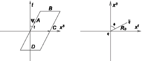
Figure 1: Configuration of the Wegner-Wilson loop in Minkowski space-time.

For the Wegner-Wilson loop in Minkowski space-time one finds from the confining field strength correlators [9]

$$<W[C]> = e^{-i\sigma R_{0}\alpha_{M}T}$$ (2)

$$\sigma = \frac{\pi^{3}G_{2}a^{2}}{18},$$ (3)

where $\sigma=0.18\,{\mbox{GeV}}^{2}$ is the string tension given by the gluon condensate $G_{2}$ and the correlation length $a$. The Minkowski-geometry enters via the factor

$$\alpha_{M}^{2}=1+\cos^{2}{\phi}\sinh^{2}{\psi}.$$ (4)

This form of the loop expectation value is consistent with the analytical continuation of the Euclidean expectation value with $\alpha=1-\cos^{2}{\phi}\sin^{2}{\theta}$ into Minkowski space by transforming the angle $\theta\rightarrow i\psi$. This analytical continuation is similar to the analytical continuation used in high energy scattering [10, 11, 12] where the angle between two Wilson loops transforms in the same way.

In addition to the contribution arising from confining field configurations there are also contributions from nonconfining field strength correlators which are derived in ref.[9] and which will be further discussed later. The exponent giving the expectation value of the Wilson loop can be related to the light cone Hamiltonian as follows. We define the four-velocity of the particles described by the tilted loop

$$u_{\mu}=(\gamma,0_{\bot},\gamma\beta).$$ (5)

and rewrite the loop with the help of the four velocity :

$$e^{-ig\int d\tau A^{\mu}u_{\mu}}=e^{-ig\int d\tau(\gamma A^{0}-\gamma\beta A^{3})}.$$ (6)

The line integral of the gauge potential acts as a phase factor on a Dirac wave function $\psi$ which splits up into a leading dynamical component $\psi_{+}$ and a dependent component $\psi_{-}$. For very fast quarks the mass term and transverse momenta are negligible compared with the energy and longitudinal momentum. In this eikonal approximation the Dirac equation of the leading component decouples from the small component:

$$i\partial_{-}\psi_{+} = P^{-}_{pot}(A^{-})\psi_{+}$$ (7)

$$= gA^{-}\psi_{+}.$$ (8)

With $\beta\approx 1$ the phase factor in the tilted Wilson loop integrates $A^{-}$ and leads to a VEV for the loop containing $P^{-}_{pot}=\frac{1}{\sqrt{2}}(P^{0}-P^{3})|_{pot}$.

$$<W_{r}[C]>=e^{-i\gamma(P^{0}-P^{3})|_{pot}T}.$$ (9)

Using eq. 1 one finds for the light cone potential energy arising from the confining part of the correlation function a term of order $O(\frac{1}{\gamma})=O(\frac{1}{P^{+}})$, where $P^{+}=\frac{1}{\sqrt{2}}(P^{0}+P^{3})$ is the light cone momentum.

$$P^{-}_{pot}=\frac{1}{\sqrt{2}}\left(\sigma R_{0}\sqrt{\cos(\phi)^{2}+\sin(\phi)^{2}/\gamma^{2}}\right).$$ (10)

Terms involving transverse momenta and masses of the same order $O(\frac{1}{P^{+}})$ are not included in the loop as it has been calculated. Two of these terms give the standard kinetic energy term of free particles, which contributes to the total light cone energy. Terms with spin cannot be obtained from this simplified derivation. We introduce the relative $+$ momentum $k^{+}$ and transverse momentum $k_{\bot}$ for the quarks with mass $\mu$. By adding the above “potential” term to the kinetic term of relative motion of the two particles we complete our approximate derivation of the light cone energy $P^{-}$

$$P^{-}=\frac{(\mu^{2}+k_{\bot}^{2})P^{+}}{2(1/4P^{+2}-k^{+2})}+\frac{1}{\sqrt{2}}\sigma\sqrt{x_{3}^{2}+x_{\bot}^{2}/\gamma^{2}}.$$ (11)

To complete the light cone Hamiltonian, we multiply $P^{-}$ with the plus component of the light cone momentum $P^{+}=\frac{1}{\sqrt{2}}(P^{0}+P^{3})$ and use that $P^{+}/M=\sqrt{2}\gamma M$ to eliminate the boost variable from the Hamiltonian. Further, we follow the notation of reference [13] and introduce the fraction $\xi=k^{+}/P^{+}$ with $|\xi|<1/2$ and its conjugate the scaled longitudinal space coordinate $\sqrt{2}\rho=P^{+}x_{3}$ as dynamical variables. For our configuration the relative time of the quark and antiquark is zero. Note that $M^{2}=2P^{+}P^{-}$.

$$H_{LC}^{q\bar{q}}(\mu^{2})=M^{2}=\frac{(\mu^{2}+\hat{k}_{\bot}^{2})}{1/4-\xi^{2}}+2\sigma\sqrt{\hat{\rho}^{2}+M^{2}x_{\bot}^{2}}.$$ (12)

We have obtained the light cone Hamiltonian $M^{2}$ from the confining interaction in a Lorentz invariant manner, because the variables $\xi,\rho,k_{\bot}$ and $x_{\bot}$ are invariant under boosts. The valence quark light cone Hamiltonian has a simple confining potential. The magnitude of the confining potential is set by the string tension $\sigma$. The effective “distance “ of the quarks is given by scale free light cone longitudinal distance and the transverse distance multiplied by the bound state mass. The dynamical variables are the light cone momentum fraction

$$\xi=k^{+}/P^{+}$$ (13)

with $|\xi|<1/2$ and its conjugate variable, namely the scaled longitudinal space coordinate

$$\sqrt{2}\rho=P^{+}x_{3}.$$ (14)

The effective “distance“ between the quarks is given by the scale-free light cone longitudinal distance $\hat{\rho}$ and the transverse distance $x_{\bot}$ multiplied by the bound state mass. Note that the transverse confinement scale is related to the self-consistent mass of the bound state $M^{2}$. In the following we will always look for solutions which obey this self consistency condition without explicitly refering to it.

The transverse momentum and the longitudinal space coordinate are represented by the operators

$$\hat{k}_{\bot}=\frac{1}{i}\vec{\nabla}_{\bot}$$ (15)

and

$$\hat{\rho}=\frac{1}{i}\frac{d}{d\xi}.$$ (16)

The above equation (12) agrees in the limit of the one-dimensional motion with the equation for the yo-yo string derived in ref. [13]. If only the transverse motion $(\rho=0)$ is present, then confinement has the usual form, which is seen by setting $M\approx 2\mu$. In general, the squared mass $\mu^{2}$ entering the Hamiltonian of eq. (12) contains the squared current quark mass $\mu_{c}^{2}$ and a quark self energy $\Delta$.

$$\mu^{2}=\mu_{c}^{2}+\Delta$$ (17)

This self energy differentiates the constituent quark from the current quark. Light fully relativistic quarks surround themselves with a cloud of gluons and quark-antiquark pairs. We will discuss the gluon part of the self energy below. For heavy quarks we will see that the self energy is negligible. One should also remark that in the light cone prescription one can not fiddle with the zero point energy of the Hamiltonian, since the Hamiltonian equals the operator for the squared mass. In the conventional nonrelativistic constituent quark Hamiltonian one always needs a sizeable negative constant $\propto 2\sqrt{\sigma}$ to get to realistic values for the groundstate energy of the meson. This negative constant will reappear as a dynamical self energy effect in the light cone Hamiltonian. One sees that a simple kinematical transformation of the nonrelativistic wave functions into light cone wave functions can never take into account such effects, since the two Hamiltonians differ in their dynamical properties.

For light quarks the stringy confining potential is the most important part and one can leave out the perturbative gluon exchange. This is not the case for the heavy quark mesons. The other non-confining potentials from the Abelian-like part of the correlator and the perturbative-gluon exchange have also been worked out from the correlation function, and one gets for the complete valence Hamiltonian [9]:

$$H_{LC}^{Q\bar{Q}}(\mu^{2}) = H_{LC}^{q\bar{q}}(\mu^{2})+H_{Yukawa}$$ (18)

$$= \frac{(\mu^{2}+\hat{k}_{\bot}^{2})}{1/4-\xi^{2}}+2\sigma r-4/3\left(\frac{2g^{2}M^{2}e^{-\frac{m_{G}r}{M}}}{4\pi r}\right)$$ (19)

with the dimensionless variable

$$r=\sqrt{\hat{\rho}^{2}+M^{2}x_{\bot}^{2}}.$$ (20)

The Yukawa-potential also comes from the stochastic vacuum model, which damps the short-range interaction at distances $r>\frac{1}{m_{G}}\approx 1/(0.77$ GeV), where the long-distance confining physics sets in. Its coupling constant $\frac{g^{2}}{4\pi}=0.81$. The same parameters have been used to calculate high-energy hadronic scattering in ref. [14]. For simplicity, we have fixed in eq. (19) the relative weights of non-perturbative non-Abelian and Abelian-like contributions by $\kappa=1.0$ compared with $\kappa=0.7$ in ref. [14], i.e. we have neglected the non-perturbative part of the correlation function, which is non-confining.

Let us now discuss the quark self energy corrections, which are especially important when the current quark masses are small. Such a self energy calculation has been discussed in the literature, also based on the stochastic vacuum model in two calculations [15, 16] cf. fig. 2. In the first version the self energy is calculated only for approximately zero current quark mass: [15]

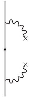
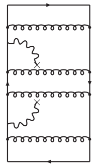
Figure 2: The left-hand diagram is a sketch of the self energy correction corresponding to [15]. The right-hand diagram shows the improved self energy correction corresponding to [16]. Crosses symbolize the color field-strength correlation functions.

$$\Delta(\mu_{c}^{2}\approx 0)=-\frac{4\sigma}{\pi}.$$ (21)

It comes out negative from the confining gluon field configurations interacting with the quark-field. In the second version [16], Simonov considers also heavy quarks with large $\mu_{c}^{2}$ and takes into account the surrounding $q\bar{q}$ state of mass $M$. Then the self energy has the form:

$$\Delta(t)=-\frac{4\sigma}{\pi}\phi(t)$$ (22)

with

$$\phi(t)=t\int_{0}^{\infty}{dzz^{2}K_{1}(tz)e^{-z}},$$ (23)

where

$$t=(\mu_{c}+M/2)a.$$ (24)

As before, $\mu_{c}$ is the current quark mass, $M$ is the uncorrected meson mass, $a=0.302$ fm is the correlation length of the field-strength correlator. The dependence of the self energy correction $\Delta(t)$ on $t$ is shown in Figure 3.

Figure 3: self energy correction $\Delta\left(\mu_{c}^{2},M\right)$ for vanishing current quark mass $\mu_{c}=0$ as a function of the uncorrected meson mass $M$.

The second self energy correction of eq. (22) agrees with the constant self energy correction of eq. (21) for $\mu_{c}=0$ and $M=0$. The self energy correction is negative for light flavours and vanishes for heavy quarks, i.e. for heavy-meson masses $M$. Such a functional behaviour looks rather reasonable. Elimination of higher $q\bar{q}$-gluon states produces an attractive interaction.

In section 4 we will adress the question of chiral symmetry breaking based on the outlined constituent quark picture. In order to do that we will parametrize the spin-spin interaction of the quarks in the meson in a rather crude way. For the spin-spin interaction we have not done any derivations and must rely entirely on a parametrization which allows us to demonstrate the effect of chiral symmetry breaking in the two body Fock space Hamiltonian. So we cannot show how the pion becomes a Goldstone boson in the light cone picture. This is a question which the constituent quark model in the nonrelativistic version has not been able to answer either.

3 Variational solution of the light cone Hamiltonian

As a first step, we evaluate the Hamiltonian for zero current quark masses $\mu_{c}^{2}=0$, with the quark self energy correction $\Delta(0)$, given by eq. (21) :

$$<\Psi|\hat{H}_{LC}^{q\bar{q}}(\Delta(0))|\Psi>=M^{2}.$$ (25)

We compute the vacuum expectation value of the Hamiltonian eq. (1), using a variational method. Simple trial wave functions factorize in a longitudinal wave function $\phi(\xi)$ and a transverse wave function $\varphi(x_{\bot})$. We take the following two trial wave functions $(i=1,2)$, where the first one has the conventional form of $\xi$-dependence:

$$\,\,\,\Psi_{i}(\xi,\vec{x}_{\bot})=\phi_{i}(\xi)\cdot\varphi(x_{\bot})\mbox{ for $i$ = 1, 2}$$ (26)

$$\,\varphi(x_{\bot})=\frac{1}{\sqrt{\pi}x_{0}}\cdot\exp\Big{[}-\frac{\vec{x}_{\bot}^{2}}{2x_{0}^{2}}\Big{]}$$ (27)

$$\mbox{with }\phi_{1}(\xi)=\sqrt{6}\cdot\left(\frac{1}{4}-\xi^{2}\right)^{1/2}$$ (28)

$$\mbox{and }\phi_{2}(\xi)=\sqrt{\frac{8}{\pi}}\cdot\left(\frac{1}{4}-\xi^{2}\right)^{1/4},$$ (29)

$x_{0}$ being the meson transverse extension of the meson.

The wave functions vanish at the kinematical boundaries $(\xi=\pm\frac{1}{2})$ which correspond to the limits of relative infinite longitudinal momenta in the non-relativistic description:

$$\Psi_{i}\left(\xi=-\frac{1}{2},x_{\bot}\right)=\Psi_{i}\left(\xi=\frac{1}{2},x_{\bot}\right)=0.$$ (30)

A non-trivial expectation value arises in the calculation of the square root operator $<\Psi|\sqrt{\hat{\rho}^{2}+M^{2}x_{\bot}^{2}}|\Psi>$. To evaluate this matrix element, we perform a Fourier transformation from $\xi$-space to $\rho$-space: The wave functions have a discrete Fourier representation due to the finite interval in $\xi$-space $\xi\in[-1/2,1/2]$:

$$\phi_{i}(\xi)=\sum_{n=-\infty}^{\infty}\tilde{\phi}_{i}(\rho_{n})\exp\left(-i\cdot\left(2n+1\right)\pi\cdot\xi\right).$$ (31)

The conjugate variable $\rho_{n}$ take the value

$$\rho_{n}=\left(2n+1\right)\pi.$$ (32)

The normalized discrete-set coefficient functions are orthogonal

$$f_{n}\left(\xi\right)=\exp\left(i\cdot\left(2n+1\right)\pi\cdot\xi\right),$$ (33)

$$\int_{-\frac{1}{2}}^{\frac{1}{2}}f_{n}\left(\xi\right)f_{m}^{*}\left(\xi\right)d\xi=\delta_{nm}.$$ (34)

Calculating the Fourier transform of the wave function $\phi_{1}(\xi)$, for example, we have

$$\tilde{\phi}_{1}(\rho_{n})=\sqrt{\frac{3}{2}}\frac{J_{1}\left(\left(n+1/2\right)\pi\right)}{2n+1}.$$ (35)

With this wave function we evaluate the expectation value of the square-root operator numerically and then approximate it by a simpler function which can be used more directly for the evaluation of the self-consistent mass $M$. The variable $y\equiv M|x_{\bot}|$ encodes the dependence of the confining interaction on the transverse extension of the bound state. We define a function $g(y)$

$$g(y)=\sum_{n=-\infty}^{\infty}\tilde{\phi}_{1}^{2}(\rho_{n})\sqrt{\rho_{n}^{2}+y^{2}},$$ (36)

which enters the complicated expectation value

$$\Big{\langle}\sqrt{\rho^{2}+M^{2}x_{\bot}^{2}}\,\Big{\rangle}=\int d^{2}x_{\bot}\,\varphi^{2}(x_{\bot})\,g(y)$$ (37)

and an approximation to $g(y)$

$$G(y)=y\left(1-\mbox{e}^{-y/a}\right)+\rho_{0}\mbox{e}^{-y^{2}/b}$$ (38)

with

$$\rho_{0}=\sum_{n=-\infty}^{\infty}\ \tilde{\phi}_{1}^{2}(\rho_{n})\rho_{n}\approx 3.53.$$ (39)

In the limit of large $y$, the exponentially decreasing terms in (38) are negligible and, because $\sum\tilde{\phi}_{1}^{2}(\rho_{n})=1$,

$$\tilde{g}(y)=y+\mathcal{O}(y^{-2}).$$ (40)

The behaviour at small $y$ constrains the parameters $a$ and $b$

$$G(y)=\rho_{0}+y^{2}\left(\frac{1}{a}-\frac{\rho_{0}}{b}\right)+\mathcal{O}(y^{3}),$$ (41)

$$\frac{1}{a}-\frac{\rho_{0}}{b}=\frac{1}{2}\sum\tilde{\phi}_{1}^{2}(\rho_{n})\frac{1}{\rho_{n}}\approx 0.15505.$$ (42)

Fitting $G(y)$ to $g(y)$ we determine $a=6.19$ and obtain from eq. (42) $b=550$. The approximate function $G(y)$ can then be integrated over the transverse space coordinate, and one gets:

$$\Big{\langle}\sqrt{\rho^{2}+M^{2}x_{\bot}^{2}}\,\Big{\rangle}\approx\frac{\rho_{0}}{M^{2}x_{0}^{2}/b+1}+\frac{\sqrt{\pi}}{2}Mx_{0}+\frac{M^{2}x_{0}^{2}}{2a}+$$ (43)

$$\frac{\sqrt{\pi}}{2}\mbox{e}^{M^{2}x_{0}^{2}/4a^{2}}\left(Mx_{0}+\frac{M^{3}x_{0}^{3}}{2a^{2}}\right)\cdot\left(\mbox{Erf}\left(\frac{Mx_{0}}{2a}\right)-1\right),$$

where Erf(x) is the error function. We repeat the same procedure for the other wave function, eq. (29). In both cases, we get self-consistent transcendental equations for $M$, which can be solved numerically. In Fig. 2, we plot the resulting masses as a function of the transverse-extension parameter $x_{0}$ of the trial wave functions $\Psi_{i}$. The trial wave function $\Psi_{1}$ leads to a smaller value of the meson mass, which lies in the expected range of light vector-meson masses. The higher mass corresponding to the trial wave function $\Psi_{2}$ comes about from the higher longitudinal momenta in this wave function. The rms-extensions $\sqrt{<x_{\bot}^{2}>}=x_{0,i}$ of the mesons can be read off from the minima of both curves. We obtain

$$x_{0,1}=0.8\,\mbox{fm}$$ (44)

and

$$x_{0,2}=0.86\,\mbox{fm}.$$ (45)

The corresponding mass values are

$$M_{1}=0.85\,\mbox{GeV}$$ (46)

and

$$M_{2}=0.89\,\mbox{GeV}.$$ (47)

Figure 4: $M(x_{0})$ for the trial wave functions $\Psi_{1}$ (full line) and $\Psi_{2}$ (dashed line). The Hamiltonian includes the self energy correction $\Delta\left(\mu^{2}=0\right)ofeq.(\ref{Simonov2001})$.

4 Chiral symmetry breaking

The method of field strength correlators is well established and we consider the presented extension of this method to the light cone another sign of its significance. We would like to differentiate from this work the purely phenomenological spin-dependent interaction which we will discuss now. In general, light mesons are influenced strongly by the spin-dependent part of the quark-antiquark interaction. It is well-known that the form of the spin-dependent interaction on the light cone is not simple and the restoration of rotational invariance on the light cone may be nontrivial. Here, we assume that this invariance can be established and introduce the spin dependent interaction on the light cone by a term $\frac{c_{q\bar{q}}}{4}\vec{\sigma}_{1}\vec{\sigma}_{2}$ which does not depend on the transverse separation nor longitudinal coordinate. We simply do not know the correct dependence. It should be short-ranged in transverse space and non-local in $\xi$ space, otherwise the spin-splitting of mesons with non-vanishing orbital momentum, like the a₁ and b₁, cannot be explained.

In order to show the effect of chiral symmetry breaking, we must make the pion mass zero for zero quark mass. To have the correct $\rho$-mass, we introduce an additional wave-function renormalization constant $Z_{\psi}$ on a purely phenomenological basis. Such a term may arise in a way similar to the Bag model [18], i.e. also on the light cone one expects Casimir corrections from the elimination of higher Fock states in the valence quark approximation. With these two parameters the theory looses any predictive power for the meson spectrum. The choice of the two parameters solely defines a good chiral symmetric starting point to study the perturbation of the chiral spectrum. It needs further investigations how the transverse and longitudinal kinetic energies get renormalized individually. We modify the Hamiltonian in the following way

$$\hat{H}=\hat{H}_{LC}^{ren}+\hat{H}_{LC}^{SS},$$ (48)

$$\hat{H}_{LC}^{ren} = \frac{\mu_{c}^{2}+\Delta(t)+Z_{\Psi}\hat{\vec{k}}_{\bot}^{2}}{(1/4-\xi^{2})}+2\sigma\sqrt{\hat{\rho}^{2}+M^{2}x_{\bot}^{2}}$$

$$\hat{H}_{LC}^{SS} = \frac{c_{q\bar{q}}}{4}\vec{\sigma}_{1}\vec{\sigma}_{2}.$$ (49)

With $Z_{\Psi}=0.4$, $\Delta(t)=-\frac{4\sigma}{\pi}\Phi(t)$ and $c_{q\bar{q}}=(0.77\,\mbox{GeV})^{2}$. As before, we start with current quark masses equal to zero. Then the squared mass of the $\rho$-meson and Goldstone mass of the $\pi$-meson are given by:

$$M_{\rho}^{2}=<\hat{H}_{LC}^{ren}>+\frac{1}{4}c_{q\bar{q}}$$ (50)

and

$$M_{\pi}^{2}=<\hat{H}_{LC}^{ren}>-\frac{3}{4}c_{q\bar{q}}.$$ (51)

Our goal now is to show that the valence picture on the light cone is consistent with chiral symmetry breaking. Chiral symmetry breaking has been a challenging aspect of light cone theory. It is known in equal-time theories that the vacuum is very complicated and higher Fock components of the quark-antiquark wave function are needed in order to reproduce the low-energy properties of the pion correctly. An interaction of the Nambu–Jona-Lasinio (NJL) type leads to a quark condensate which is spread out over all space. Such condensates are contrary to the naive light cone picture of a trivial vacuum. The excitations of this condensate are massless Goldstone pions. In the light cone approach, the most developed calculation uses the NJL-model with a vector interaction [17] and obtains very interesting differences of the light cone wave function between the vector mesons and pions. In our framework, the complicated self energy correction $\Delta(t)$ of the constituent quark can give the correct chiral-symmetry behaviour of the pion mass. We apply the Feynman-Hellmann theorem [19] to the light cone Hamiltonian, which has dimension $[\mbox{mass}]^{2}$

$$\frac{\partial M_{\pi}^{2}}{\partial\mu_{c}}=\Big{<}\frac{\partial\hat{H}}{\partial\mu_{c}}\Big{>}$$ (52)

and investigate what happens to the $\pi$-mass squared $M_{\pi}^{2}=0$, when the current quark mass $\mu_{c}$ increases to finite values $\mu_{c}\not=0$. Especially one may ask whether the Gell-Mann–Oakes–Renner relation still holds. How can the pion mass squared vanish linearly with the quark mass? A naive kinetic term cannot do that because then $\Delta M_{\pi}^{2}\propto\mu_{c}^{2}$. In the Hamiltonian $\hat{H}$ (49) with $\Delta(t)$ we have, however,

$$\frac{\partial M_{\pi}^{2}}{\partial\mu_{c}}\Big{|}_{\mu_{c}=0}=\frac{-\frac{4\sigma}{\pi}\left<\frac{1}{1/4-\xi^{2}}\right>\frac{\partial\phi(t)}{\partial\mu}\Big{|}_{t=(M_{0}/2)\,a}}{1-\sigma<\frac{x_{\bot}^{2}}{\sqrt{\rho^{2}+M^{2}x_{\bot}^{2}}}>}\,.$$ (53)

The t-dependence of $\Delta(t)$ cf. eq. (22) influences the expectation value of $\hat{H}$, which is evaluated with $\Psi_{1}$ of eq. (26). For $M_{0}$ we take the averaged meson mass of $<\hat{H}_{LC}^{ren}>$ and for the transverse extension we have  $x_{0}=0.8\,\mbox{fm}$. We get a linear dependence of the square of the pion mass on the quark mass with a positive slope which is related to the behaviour of the quark self energy when one goes from light quark systems to heavy quark systems. It is naturally positive, because the quark self energy starts with a negative value for the light quarks and becomes zero for heavy quarks.

$$\frac{\partial M_{\pi}^{2}}{\partial\mu}\Big{|}_{\mu=0}\approx 3.38\,\,\mbox{GeV}.$$ (54)

When we compare this value with the one from the Gell-Mann–Oakes–Renner relation [20, 21]

$$M_{\pi}^{2}/\mu=-2\frac{<0|\bar{q}q|0>}{F_{\pi}^{2}}\ \approx 3.20\,\,\mbox{GeV},$$ (55)

we only find a small difference between our light cone calculation of eq. (54) and the empirical value $\frac{\partial M^{2}}{\partial\mu}$ of eq. (55).For the absolute value of the quark condensate we took $(-0.240\,\,\mbox{GeV})^{3}$ and $F_{\pi}=0.093$ GeV [22]. This result due to the self energy correction $\Delta(t)$ asks for further studies of the self energy correction in the light cone theory. Here, new possibilities are opening up in the AdS/QCD approach [23, 24]. However, it should be mentioned that the quark condensate is scheme and renormalization scale dependent, i.e. eq. (55) is very sensitive to small changes of the quark condensate.

5 Heavy quarks

For heavy quarks, chiral symmetry is not relevant, but the short-range interaction $\hat{H}_{Yukawa}$ can be tested. In the derivation with field strength correlators, it comes about from the perturbative Abelian field strength correlator which dominates the short distances and fades out at large distances $r>\frac{1}{m_{G}}\approx 1/(0.77$ GeV). The coupling constant $\frac{g^{2}}{4\pi}=0.81$ of this “Yukawa” part of the potential is taken over from the successful high energy calculations of hadron-hadron scattering and e-p scattering at Hera energies [14]. We can test its magnitude and form comparing with the mass spectrum of heavy quarks. For heavy quarks we have $\hat{H}_{LC}^{Q\bar{Q}}=\hat{H}_{LC}^{ren.}+\hat{H}_{LC}^{SS}+\hat{H}_{Yukawa}$:

$$\hat{H}_{LC}^{Q\bar{Q}}=\underbrace{\frac{\mu_{c}^{2}+Z_{\Psi}\hat{\vec{k}}_{\bot}^{2}}{(1/4-\xi^{2})}+2\sigma\sqrt{\hat{\rho}^{2}+M^{2}x_{\bot}^{2}}}_{\hat{H}_{LC}^{ren.}}+\underbrace{\frac{c_{Q\bar{Q}}}{4}\vec{\sigma}_{1}\vec{\sigma}_{2}}_{\hat{H}_{LC}^{SS}}\underbrace{-4/3\left(\frac{2g^{2}M^{2}e^{-\frac{m_{G}r}{M}}}{4\pi r}\right)}_{\hat{H}_{Yukawa}}.$$ (56)

Let us take the charmonium system as an example. The charm mass is chosen as $\mu_{c}^{2}=1.82\,~{}GeV^{2}$ and the self energy $\Delta(t)$ vanishes for heavy quarks as shown in fig. (3). The wave function renormalization of the heavy quark can be chosen the same as for the light quark, which means that the higher Fock states eliminated in the valence approximation have approximately the same lower threshold. In other words, the important contributions come from higher orbital excitations or quark gluon states which lie well above the charm quark mass. In Fourier space the variable $r$ in the light cone Hamiltonian has a purely algebraic form without any differential operator,

$$r=\sqrt{\rho_{n}^{2}+M^{2}{\vec{x}_{\bot}}^{2}}.$$ (57)

Therefore, the normalized wave function $\Psi_{1}$ in the Fourier representation depends on $\rho_{n}=(2n+1)\pi$ and $x_{\bot}$.

$$\Psi_{1}(\xi,\vec{x}_{\bot})=\sum_{n=-\infty}^{\infty}\underbrace{\tilde{\phi}_{1}(\rho_{n})\varphi(x_{\bot})}_{\equiv\tilde{\Psi}_{1}(\rho_{n},\vec{x}_{\bot})}e^{-i\rho_{n}\xi}$$ (58)

$$\tilde{\Psi}_{1}(\rho_{n},\vec{x}_{\bot})=\tilde{\phi}_{1}(\rho_{n})\cdot\varphi(x_{\bot})=\sqrt{\frac{3}{2}}\frac{J_{1}((n+\frac{1}{2})\pi)}{2n+1}\frac{1}{\sqrt{\pi}x_{0}}\exp{\Big{[}-\frac{\vec{x}_{\bot}^{2}}{2x_{0}^{2}}\Big{]}},$$ (59)

where $\tilde{\phi}_{1}(\rho_{n})$ is given by eq. (35). Because of the factorizing ansatz, we can split the evaluation of the “Yukawa” interaction into two steps: First, we average over the continuous $\vec{x}_{\bot}$-dependent part of the wave function

$$a_{n}\equiv<\varphi|\hat{H}_{Yukawa}|\varphi>=-\frac{2}{3\pi}g^{2}M^{2}\exp{\Big{[}\frac{(\pi+2\pi n)^{2}}{M^{2}x_{0}^{2}}+\frac{m_{G}^{2}x_{0}^{2}}{4}\Big{]}}$$ (60)

$$\times\frac{\sqrt{\pi}}{Mx_{0}}\mbox{Erfc}\left[\frac{\sqrt{(\pi+2\pi n)^{2}}}{Mx_{0}}+\frac{m_{G}x_{0}}{2}\right].$$

Secondly, we sum over the discrete Fourier components. We write the second averaging process in the form

$$<<\hat{H}_{Yukawa}>>=\sum_{n=-\infty}^{\infty}a_{n}\tilde{\phi}_{1}(\rho_{n})^{2}\approx\sum_{n=-5}^{5}a_{n}\tilde{\phi}_{1}(\rho_{n})^{2}.$$ (61)

In practice, we truncate the infinite sum in eq. (61) by the first 11 leading terms. The proof of convergence of eq. (61) is given in Appendix A. As one can see in Fig. 4, the Yukawa interaction lowers the charmonium mass by about 220 MeV. The spin averaged mass of the 1$s-c\bar{c}$ state comes out as $<\hat{H}_{LC}^{ren.}+\hat{H}_{Yukawa}>=3.06$ GeV with the same wave-function renormalization factor $Z_{\psi}\approx 0.4$ for the kinetic term of the Hamiltonian as we used before. The size of the transverse-extension parameter for 1$s$-charmonium is much smaller, $x_{0}=0.3\,\mbox{fm}$. As one sees, the valence-quark Hamiltonian can be made also a reliable instrument for heavy-quark spectroscopy. Since we kept the wave function renormalization, the spin averaged mass for the heavy quarks is a prediction. The masses of the $\psi$ and $\eta_{c}$ mesons can be fitted with a value:

$$c_{Q\bar{Q}}/4=0.18GeV^{2}.$$ (62)

This value is about the same as the light quark parameter $c_{q\bar{q}}/4=0.15GeV^{2}$. The corresponding heavy light systems D${}_{0}^{*}$/D₀ and B${}_{0}^{*}$/B₀ have approximately similar splittings with $c_{Q\bar{q}}/4=0.15\,\text{GeV}^{2}$(D) and $0.12\,\text{GeV}^{2}$(B). Thus the strength of the spin-spin interaction added to the square of the mass operator seems to be largely flavor blind.

Figure 5: $M(x_{0})$ from $H_{LC}+\hat{H}_{Yukawa}$ (full line) and from the Hamiltonian of eq. (12) without Coulomb interaction (dashed line). We use as a trial wave function $\Psi_{1}$ given by eq. (26).

6 Conclusion

Gluon field-strength correlators yield the most important confining interaction of the light cone constituent Hamiltonian derived in ref. [9]. Extending the range of applications of this Hamiltonian, we have calculated in this paper light and heavy meson masses and wave functions. Let us retrace the most important parts of our calculation.

We have added to the Hamiltonian of ref. [9] a negative self energy correction $\Delta$, which also has been calculated in the framework of the gluon field strength correlators [15, 16]. This self energy is necessary to obtain reasonable light meson masses. The improved form of the self energy correction varies with the uncorrected meson mass and vanishes for large meson masses, i.e. for large quark masses. The self energy correction comes about from non-perturbative binding corrections inside the meson. The dependence of $\Delta(t)$ on the current quark mass is crucial to obtain the correct symmetry pattern for the pion mass. To get to zero pion mass for zero current quark mass, a phenomenological spin-spin interaction is necessary. For charmonium the “Yukawa” part of the $Q\bar{Q}$ interaction from the Abelian-like field-strength correlator is relevant. It is important that the purely phenomenological parameters do not vary much for both light and heavy systems. Our variational calculations are based on trial wave functions which factorize. This is not necessary. Extending the set of basis functions we found a small variation of the mean transverse momentum with the longitudinal momentum. Further work is needed to find out theoretically the spin-spin interaction and the wave function renormalization.

The framework of the light cone Hamiltonian proposed here has to be seen in context with the successful parametrization of high-energy hadron-hadron scattering based on the same gluon-field strength correlation functions ref. [14]. Until now, the dipole approach uses only phenomenological light cone wave functions for the asymptotic hadronic states. The propagation of a color dipole in the nucleus demands a dynamical treatment [25]. The dipole propagates with an imaginary potential due its inelastic scatterings and with a real potential which confines the quarks on their way through the nucleus. Its Greens-function determines the shadowing of nuclear structure functions or heavy quark production in nuclei. Our approach may help to formulate this problem consistently. With this work, we converge towards a unified description of QCD bound states and hadronic scattering which has been a long term goal of QCD.

Acknowledgments: We thank D. Antonov and J.-P. Lansberg for a reading of the manuscript and helpful discussions.

7 Appendix

Appendix A Proof of finiteness of $<<\hat{H}_{Yukawa}>>$

To prove the convergence of the sum for $<<\hat{H}_{Yukawa}>>$ in eq. $(\ref{Sum})$ we will use the Abelian convergence test ref. [26]. This test says: Let $\{{x_{n}}\}$ and $\{{y_{n}}\}$ be two sequences of real numbers. If

$$\,\,\,\sum_{n=1}^{\infty}x_{n}\neq\infty$$ (63)

$$\,\,\,y_{n+1}\,\leq\,y_{n}$$ (64)

$$\,\,\,\lim_{n\rightarrow\infty}y_{n}\neq\infty$$ (65)

then $\sum_{n=1}^{\infty}x_{n}y_{n}$ converges.

Now we apply this convergence test to $<<\hat{H}_{Yukawa}>>$. We identify $x_{n}\equiv a_{n}$ with $a_{n}$ of eq. (60)  and $y_{n}\equiv(\tilde{\phi}_{1}(n))^{2}$ with $\tilde{\phi}_{1}(n)$ of eq. (35), and split $<<\hat{H}_{Yukawa}>>$ into $\sum_{n=1}^{\infty}x_{n}y_{n}$ and $\sum_{n=1}^{\infty}x_{-n}y_{-n}$.


For $M\neq 0$ and $M\neq\infty$ we have $0<r<1$ with

$$r:=\lim_{n\rightarrow\infty}\sqrt[n]{x_{n}}=\exp{\Big{[}-\frac{2m_{G}\pi}{M}\Big{]}}<1.$$ (66)

According to the Root test $\sum_{n=1}^{\infty}x_{n}$ fulfills the first condition eq. (63).

Since $\tilde{\phi}_{1}(n+1)\leq\tilde{\phi}_{1}(n)$ $\{y_{n}\}$ is decreasing and fulfills eq. (64). $\lim_{n\rightarrow\infty}\tilde{\phi}_{1}(n)=0$ implies $\lim_{n\rightarrow\infty}y_{n}\neq\infty$ (eq. 65). Therefore, conditions eq. (63, 64, 65) are fulfilled and $\sum_{n=-\infty}^{\infty}x_{n}y_{n}$ converges.

References

- [1] S. Simula, Phys. Rev. C 66 (2002) 035201 [arXiv:nucl-th/0204015].
- [2] A. Yu. Dubin, A. B. Kaidalov and Yu. A. Simonov, Phys. Lett. B 343 (1995) 310.
- [3] M. Burkardt and S. Dalley, Prog. Part. Nucl. Phys. 48 (2002) 317 [arXiv:hep-ph/0112007].
- [4] S. Dalley and B. van de Sande, Phys. Rev. D 67 (2003) 114507 [arXiv:hep-ph/0212086].
- [5] T. Frederico, H. C. Pauli and S. G. Zhou, Phys. Rev. D 66 (2002) 116011 [arXiv:hep-ph/0210234].
- [6] A. Di Giacomo, H. G. Dosch, V. I. Shevchenko and Yu. A. Simonov, Phys. Rept. 372 (2002) 319 [arXiv:hep-ph/0007223].
- [7] O. Nachtmann, arXiv:hep-ph/9609365.
- [8] A.I. Shoshi, F.D. Steffen, H.G. Dosch and H.J. Pirner, Phys. Rev. D 68 (2003) 074004.
- [9] H. J. Pirner and N. Nurpeissov, Phys. Lett. B 595 (2004) 379 [arXiv:hep-ph/0404179].
- [10] E. Meggiolaro, Z. Phys. C 76 (1997) 523 [arXiv:hep-th/9602104].
- [11] E. Meggiolaro, Nucl. Phys. B 625 (2002) 312 [arXiv:hep-ph/0110069].
- [12] A. Hebecker, E. Meggiolaro and O. Nachtmann, Nucl. Phys. B 571 (2000) 26 [arXiv:hep-ph/9909381].
- [13] W. A. Bardeen, I. Bars, A. J. Hanson and R. D. Peccei, Phys. Rev. D 13 (1976) 2364.
- [14] A.I. Shoshi, F.D. Steffen and H.J. Pirner, Nucl. Phys. A 709 (2002) 131.
- [15] Yu. A. Simonov, Phys. Lett. B 515 (2001) 137 [arXiv:hep-ph/0105141].
- [16] Yu. A. Simonov, Phys. Atom. Nucl. 68 (2004) [arXiv:hep-ph/0407027].
- [17] K. Naito, S. Maedan and K. Itakura, Phys. Rev. D 70 (2004) 096008 [arXiv:hep-ph/0407133].
- [18] S. N. Goldhaber, R. L. Jaffe and T. H. Hansson, Nucl. Phys. B 277 (1986) 674.
- [19] R. P. Feynman, Stat. Mechanics . A set of lectures (Addison-Wesley Publishing Co. Inc., The Advanced Book Program, Reading, Massachusetts, 1972).
- [20] J. F. Donoghue, E. Golowich and B. R. Holstein, Camb. Monogr. Part. Phys. Nucl. Phys. Cosmol. 2 (1992) 1.
- [21] M. Gell-Mann, R. J. Oakes and B. Renner, Phys. Rev. 175 (1968) 2195.
- [22] P. Salabura et al. [HADES Collaboration], Acta Phys. Polon. B 35, 1119 (2004).
- [23] S. J. Brodsky and G. F. de Teramond, arXiv:0802.0514 [hep-ph].
- [24] O. Andreev and V. I. Zakharov, Phys. Rev. D 74 (2006) 025023 [arXiv:hep-ph/0604204].
- [25] B. Z. Kopeliovich, J. Raufeisen and A. V. Tarasov, Phys. Rev. C 62 (2000) 035204 [arXiv:hep-ph/0003136].
- [26] T. J. Bromwich, An Introduction to the Theory of Infinite Series, MacMillan & Co. 1908, revised 1926, reprinted 1939, 1942, 1949, 1955, 1959, 1965.