Information theoretic bounds for Compressed Sensing

Abstract

In this paper we derive information theoretic performance bounds to sensing and reconstruction of sparse phenomena from noisy projections. We consider two settings: output noise models where the noise enters after the projection and input noise models where the noise enters before the projection. We consider two types of distortion for reconstruction: support errors and mean-squared errors. Our goal is to relate the number of measurements, $m$, and SNR, to signal sparsity, $k$, distortion level, $d$, and signal dimension, $n$.

We consider support errors in a worst-case setting. We employ different variations of Fano’s inequality to derive necessary conditions on the number of measurements and SNR required for exact reconstruction. To derive sufficient conditions we develop new insights on max-likelihood analysis based on a novel superposition property. In particular this property implies that small support errors are the dominant error events. Consequently, our ML analysis does not suffer the conservatism of the union bound and leads to a tighter analysis of max-likelihood. These results provide order-wise tight bounds. For output noise models we show that asymptotically an SNR of $\Theta(\log(n))$ together with $\Theta(k\log(n/k))$ measurements is necessary and sufficient for exact support recovery. Furthermore, if a small fraction of support errors can be tolerated, a constant SNR turns out to be sufficient in the linear sparsity regime. In contrast for input noise models we show that support recovery fails if the number of measurements scales as $o(n\log(n)/SNR)$ implying poor compression performance for such cases.

Motivated by the fact that the worst-case setup requires significantly high SNR and substantial number of measurements for input and output noise models, we consider a Bayesian setup. To derive necessary conditions we develop novel extensions to Fano’s inequality to handle continuous domains and arbitrary distortions. We then develop a new max-likelihood analysis over the set of rate distortion quantization points to characterize tradeoffs between mean-squared distortion and the number of measurements using rate-distortion theory. We show that with constant SNR the number of measurements scales linearly with the rate-distortion function of the sparse phenomena.

1 Introduction

In this paper we derive information theoretic bounds on the performance of the Compressed Sensing problem, [1],[2],[3],

$$\mathbf{Y}=\mathbf{G}\mathbf{X}+\frac{\mathbf{N}}{\sqrt{\textit{SNR}}}$$ (1)

where the measurements $\mathbf{Y}\in\mathbb{R}^{m\times 1}$, the desired signal $\mathbf{X}\in\mathbb{R}^{n}$, and the compression (sensing) matrix $\mathbf{G}\in\mathbb{R}^{m\times n}$. The noise $\mathbf{N}\stackrel{{\scriptstyle d}}{{\sim}}{\cal N}(0,\mathbf{I}_{m})$, where $\mathbf{I}_{m}$ is an identity matrix of size $m$, is assumed to be a Gaussian random vector with independent identically distributed (IID) components. We characterize results for both deterministic and stochastic compression matrices $\mathbf{G}=[g_{ij}]$. For deterministic, $\mathbf{G}$, the columns, $\mathbf{g}_{j}$, are normalized to have unit $\ell_{2}$ norm. For the stochastic setting we consider matrices drawn from IID (independent identically distributed) Gaussian ensembles. Each component here is assumed to be distributed as $g_{ij}\stackrel{{\scriptstyle d}}{{\sim}}{\cal N}(0,1/m),\,\,\,i=1,\,\ldots,m,\,j=1,2,\ldots,\,n$. Note that under this normalized sensing matrix scenario, the term SNR also denotes the inverse of the noise variance. We refer to the signal model of Equation (1) as the output noise model. In parallel we also consider the input noise model given by,

$$\mathbf{Y}=\mathbf{G}\left(\mathbf{X}+{\mathbf{N}\over\sqrt{\textit{SNR}}}\right)$$ (2)

where $\mathbf{N}\stackrel{{\scriptstyle d}}{{\sim}}{\cal N}(0,\mathbf{I}_{n})$ is a Gaussian random vector with IID components. Evidently the noise here enters before the “compression” operator, $\mathbf{G}$, is applied. This model is motivated by fusion problems that arise in sensor networks [4], where noisy observations are compressed.

The support of the signal $\mathbf{X}$ is denoted by $\mbox{Supp}(\mathbf{X})=\{j\mid X_{j}\not=0\}$. We assume that the cardinality of the signal support, $|\mbox{Supp}(\mathbf{X})|\leq k<n$. It is often convenient to state and interpret results in terms of the sparsity ratio $\alpha_{n}=\frac{k}{n}$. The regime when $\alpha_{n}\stackrel{{\scriptstyle n\rightarrow\infty}}{{\longrightarrow}}\alpha>0$ is referred to as the linear regime and the regime when $\alpha_{n}\stackrel{{\scriptstyle n\rightarrow\infty}}{{\longrightarrow}}0$ is referred to as the sub-linear regime.

We consider two types of distortions in signal reconstruction, namely, (a) Support distortion, i.e., $d(\hat{\mathbf{X}},\mathbf{X}))=\frac{1}{k}\sum_{j=1}^{n}|I_{\{X_{i}\not=0\}}-I_{\{\hat{X}_{i}\not=0\}}|$, where, $I_{\{\cdot\}}$ is the indicator function. (b) Mean squared distortion, $d(\hat{\mathbf{X}},\mathbf{X}))=\frac{1}{n}\|\hat{\mathbf{X}}-\mathbf{X}\|^{2}=\frac{1}{n}\sum_{j=1}^{n}|\hat{X}_{j}-X_{j}|^{2}$. These two distortion metrics address two different issues in signal recovery. The first metric penalizes solely the support detection part while the second metric penalizes both support detection and amplitude estimation. We will now highlight the main contributions and results of the paper.

1.1 Bounds for Exact and Approximate Support Recovery

In this part we further restrict the signal $\mathbf{X}$ to be bounded away from zero by a constant $\beta>0$ on its support. This is a standard assumption employed by other researchers(see [5, 6, 7, 8]) since it is impossible to identify the support of a signal $\mathbf{X}$ from noisy measurements with arbitrarily small non-zero components. We derive necessary and sufficient conditions for exact and approximate support recovery for this case under both output and input noise models. A central contribution of our work in this setting is that we explicitly quantify the required SNR and the number of measurements, $m$ for exact support recovery. For the output noise model we show that the minimum SNR required for support recovery is $\Omega(\log(n))$ regardless of $m$. In addition for this minimum SNR level, the number of measurements, $m$, must scale as $\Omega(k\log(n/k))$ to guarantee exact support recovery. Furthermore, we derive sufficient conditions and show that with $\textit{SNR}=\Omega(\log(n))$ and $m=\Omega(k\log(n/k))$ the maximum-likelihood decoder can exactly identify the signal support with high probability. These results are depicted in Table 1. While not depicted in this table it is interesting to consider what happens as SNR increases. The bounds derived in this paper show that we cannot get significant improvement in $m$ unless SNR is scaled substantially (as a fractional power of $n$). We also derive conditions for support recovery for input noise models. Here our necessary conditions say that if $m=o\left({n\log(n)\over\textit{SNR}}\right)$ then recovery would be impossible. Evidently, either the SNR or the number of measurements must scale linearly with $n$ to ensure support recovery. Thus either we must operate in an essentially noiseless regime or forsake all compression. We also extend our results to approximate support recovery. Here a tradeoff between the number of measurements, SNR and support errors for different sparsity ratios. These tradeoffs are summarized in Column 2 of Table 2. An interesting aspect of these results is that a constant SNR is sufficient if we could tolerate a constant fraction of errors in the support recovery. To establish the necessary conditions we use Fano’s inequality and its variations [9]. For deriving sufficient conditions we analyze the performance of the Maximum-Likelihood (ML) estimator based on a novel insight that every large support error event is essentially contained in the union of single support error events. This leads to a sharp bound that is order-wise optimal. Our necessary and sufficient conditions for different sparsity levels require similar scaling of SNR, and the number of measurements(see Table 1).

Related Literature- The necessary condition that $\textit{SNR}=\Omega(\log(n))$ irrespective of the number of measurements was first reported by the authors in [10]. This paper extends these results to include necessary conditions on the number of measurements. Similar conditions have also been reported by Fletcher et. al. [11] but due to the constraints imposed on the signal space—the signal is limited to have small amplitude variations on its support elements—their conditions are conservative (see discussion in [5]) for our setup. Necessary conditions have also been derived by Wainwright [6]. When the bounds of [6] (see Theorem 2 in [6]) are applied to our setup, it implies that the number of measurements scale as $\Omega(\log(n))$, which is conservative. In addition [6], primarily imposes conditions on the number of measurements but does not impose separate bounds on SNR. In contrast we show that unless SNR scales as $\Omega(\log(n))$ support recovery is impossible regardless of $m$. Furthermore, for $\textit{SNR}=O(\log(n))$ we show that $m$ must scale as $\Omega(k\log(n/k))$. Sufficient conditions for support recovery for output noise models has been described in [6, 12, 11, 7, 8] as well. Nevertheless, these upper bounds are also significantly weaker than that appearing here. Both Wainwright [6] and Akcakaya et. al. [12] use union bounding to derive error bounds for exact recovery. Union bounds are generally conservative and results in requiring significantly high SNR, i.e. significantly low admissible noise variance (see for instance, Theorem 1 in [6]). The sufficient conditions of Fletcher et. al. [11] is based on Greedy Basis Pursuit algorithm. However, their analysis, as described earlier, constrains the signals, $\mathbf{X}$, to have small amplitude variations on its support elements and when applied to our output noise setup is conservative (see again discussion in [5]). While [13, 12] derive some results for approximate support recovery, the achievable region in terms of number of measurements and SNR as a function of achievable distortion is implicitly stated and is therefore not comparable to the results presented here.

EXACT SUPPORT RECOVERY (Output Noise Model)
	Linear Sparsity	Sub-Linear Sparsity
	$0<\alpha=\alpha_{n}=\frac{k}{n}$	$\alpha_{n}=\frac{k}{n}=n^{-\gamma},\,\,\gamma>0$
Necessity (this paper)	$\textit{SNR}=\Omega\left({\log(n)\over\beta^{2}}\right)$	$\textit{SNR}=\Omega\left({\log(n)\over\beta^{2}}\right)$
	$m=\Omega(n)$	$m=\Omega(k\log\frac{n}{k})$
Sufficiency (this paper)	$\textit{SNR}={32\log(2n)\over\beta^{2}}$	$\textit{SNR}={32\log(2n)\over\beta^{2}}$
	$m=6nH_{2}(2\alpha)$, $\alpha\leq 0.04$	$m=6k\log\frac{n}{2k}$

Table 1: Summary of fundamental bounds for exact support recovery in the worst-case setting described in Equation (1). $\beta$ is the minimum absolute value of the signal $\mathbf{X}$ on its support set; $H_{2}(\cdot)$ denotes the binary entropy function; $k$ is the maximum allowable cardinality (sparsity) of the support of $\mathbf{X}$; $\alpha$ is the maximum sparsity ratio and; $1/\textit{SNR}$ is the noise variance in each noise dimension. The necessary conditions are stated for arbitrary (not necessarily IID) matrices, $\mathbf{G}$, such that the marginal distribution of each component has zero mean and variance $1/m$. The sufficient conditions are stated for the case when each element of $\mathbf{G}$ is drawn IID $\sim{\cal N}(0,\frac{1}{m})$.

1.2 Rate distortion bounds

In the second part of the paper, we consider sparse Bayesian signal models for $\mathbf{X}$ to fully exploit the power of information theoretic methods. This naturally leads us to characterizing necessary and sufficient conditions in terms of the rate distortion function.

We first consider arbitrary pointwise distortion metrics, i.e., $\frac{1}{n}d(\hat{\mathbf{X}},\mathbf{X})=\frac{1}{n}\sum_{j}d(\hat{X}_{j},X_{j}),\,\,j=1,\,2,\,\ldots,\,n$, where $X_{j},\,\hat{X}_{j}$ are the j-th components of $\mathbf{X},\,\hat{\mathbf{X}}$ respectively. For deriving necessary conditions we develop a new modified Fano’s inequality that provides us with a worst case lower bound to the probability of error in reconstruction to within a distortion $\frac{1}{n}d(\hat{\mathbf{X}},\mathbf{X})\leq d_{0}$ in terms of the scalar rate distortion function $R_{X}(d_{0})$ and mutual information $\mathbb{I}(\mathbf{X},\mathbf{Y})$, between $\mathbf{X}$ and $\mathbf{Y}$. This bound is of independent interest since it can be applied to non-sparsifying distributions as well. In particular we show that,

$$\mathbb{P}\left(\frac{1}{n}d(\hat{\mathbf{X}},\mathbf{X})\geq d_{0}\right)\geq\dfrac{R_{X}(d_{0})-c_{0}-\frac{1}{n}\mathbb{I}(\mathbf{X};\mathbf{Y})}{R_{X}(d_{0})}$$

for some small constant $c_{0}<R_{X}(d_{0})$.

For deriving sufficient conditions we compute upper bounds to the probability of error subject to a tolerable distortion based on the so called covering property of rate distortion theory. In particular we formalize a minimum distance decoder (distance measured in terms of given distortion metric) over the set of rate distortion quantization points. We then specialize our bounds to the mean squared distortion metric. The results are summarized in the second column of Table 2. Our necessary and sufficient conditions for the number of measurements and SNR match within a constant factor for the linear sparsity regime.

Related Literature- Rate distortion analysis has been reported in [14, 15] for mean squared error and for a Gaussian source. In contrast our expressions apply to general distortion measures and to any source for which a rate distortion function is defined. These results appeared in our preliminary work [16]. In addition the results in [14] for the case when $\mathbf{G}$ is random are only proven for $k=1$. In contrast in this paper we prove results for general $k=\alpha n$. For a fixed problem size $(n,k,m)$ the results in [15] are stated in terms of a critical SNR threshold. This makes the expressions implicit in the number of measurements required as a function of signal sparsity and therefore the scaling laws are unclear.

APPROXIMATE SUPPORT RECOVERY - Sufficient conditions (Linear Sparsity Regime)
Support Error Distortion $\frac{1}{k}\sum_{j=1}^{n}|I_{\{X_{i}\not=0\}}-I_{\{\hat{X}_{i}\not=0\}}|\leq d_{0}$	Mean Squared Distortion $\frac{1}{n}\|\hat{\mathbf{X}}-\mathbf{X}\|^{2}\leq d_{0}$
$\textit{SNR}=\Omega\left(\frac{H_{2}\left(2\alpha_{n}d_{0}\right)}{\beta^{2}}\right)$ and $m=\Omega(nH_{2}(2\alpha_{n}))$	$m=\Omega(nR_{X}(d_{0}/2))$, for $\textit{SNR}=\Omega(\frac{R_{X}(d_{0}/2)}{d_{0}})$.

Table 2: The first column describes the achievable rate regions for approximate support recovery. Support error distortion $d_{0}$ is the fraction of the true support in error. The second column describes the results for the Bayesian set-up in terms of the scalar rate distortion function for varying mean squared distortion. Here the distortion $d_{0}$ is the desired mean-squared-distortion.

The rest of the paper is organized as follows. In Section 2 we present our problem set-up. Here the notion of Sensing Capacity is introduced to study the asymptotic behavior of both the output noise and input noise models. Section 3 presents necessary and sufficient conditions for support recovery. In Section 4 we consider the Bayesian setup and derive bounds for signal recovery under arbitrary distortion measures. This requires us to generalize the traditional Fano’s inequality to general (average) distortion measures and continuous signal spaces. We also provide extensions of Fano’s inequality for discrete signal spaces with Hamming distortion in reconstruction. Section 4.2 presents a novel ML upper bound for signal recovery to within a given squared distortion level. Using these results, in Section 5 we evaluate bounds for SNR and number of measurements required to reconstruct $\mathbf{X}$ to different levels of distortion level for output and input noise models. We then comment on the differences between worst-case and Bayesian setups.

2 Problem Set-up

We consider output and input noise models described in Equations (1) and (2). The sparsity of $\mathbf{X}$ is modeled both deterministically and stochastically as is the compression matrix $\mathbf{G}$. We use bold-face to denote vectors and matrices, while regular font is used to denote scalar components of the vector and matrices. The jth component of a vector $\mathbf{X}$ is denoted $X_{j}$, the jth column of a matrix $\mathbf{G}$ is denoted $\mathbf{g}_{j}$ and its ij-th component is denoted as $g_{ij}$. The cardinality of a set $S$ is denoted by $|S|$. Given a set $S\subset\{1,\,2\,\ldots,\,n\}$, $\mathbf{X}_{S}$ denotes the signal, $\mathbf{X}$, restricted to the set of components indexed by $S$. Similarly, we denote by $\mathbf{G}_{S}$ the matrix formed from columns indexed by $S$. We use $\Pr(\cdot)$ and $\mathbb{P}(\cdot)$ interchangeably to denote the probability of an event.

Non-Random Sparsity Signal Model:

We say that $\Xi^{\{k\}}\subset\mathbb{R}^{n}$ is a family of k-sparse sequences if for every $\mathbf{X}\in\Xi^{\{k\}}$, the support of $\mathbf{X}$ is smaller than or equal to $k$. Formally, let

$$\mbox{\mbox{Supp}}(\mathbf{X})=\{j\mid X_{j}\not=0\}$$

Then $\Xi^{\{k\}}$ is a family of k-sparse sequences if,

$$\Xi^{\{k\}}=\left\{\mathbf{X}:|\mbox{Supp}(\mathbf{X})|\leq k\right\}$$ (3)

We will refer to the ratio, $\alpha_{n}=k/n$ as the sparsity ratio. We will often work with subsets of $\Xi_{\beta}^{\{k\}}\subset\Xi^{\{k\}}$. These are sequences whose minimum absolute value is bounded away from zero by a constant $\beta\geq 0$:

$$\Xi_{\beta}^{\{k\}}=\{\mathbf{X}\in\mathbb{R}^{n}:|\text{Supp}(\mathbf{X})|\leq k,\,\,|X_{j}|\geq\beta,\,\,\,\forall\,j\in\mbox{Supp}(\mathbf{X})\}$$ (4)

We will see when we derive necessary conditions that $\beta>0$ is necessary for support recovery. This is mainly because it is impossible to determine the support of a signal with arbitrarily small components under noisy measurements. This condition is also assumed by other authors [17, 7].

We denote by $\Xi^{k}\subset\Xi^{\{k\}}$ the set consisting of exactly k-sparse sequences.

$$\Xi^{k}=\left\{\mathbf{X}:|\mbox{Supp}(\mathbf{X})|=k\right\}$$ (5)

This distinction is important and the reader should keep this in mind. The subset $\Xi_{\beta}^{k}\subset\Xi^{k}$ is analogously defined.

Bayesian signal model:

We say that a prior distribution on $\mathbf{X}$ is an asymptotically sparsifying distribution if for sufficiently large $k,n$ the distribution concentrates all the measure on a subset of $\Xi^{\{k\}}$. In this paper we will provide general results for arbitrary sparsifying priors and explicit bounds for the following Gaussian mixture model, namely, each component of the signal is distributed as:

$$X_{i}\stackrel{{\scriptstyle d}}{{\sim}}P_{X}=\alpha{\cal N}(\mu_{1},\sigma_{1}^{2})+(1-\alpha){\cal N}(\mu_{0},\sigma_{0}^{2})$$

The corresponding $n$ dimensional distribution of $\mathbf{X}$ is realized as a product measure on $\mathbb{R}^{n}$. As an example note that for $\mu_{1}=1,\mu_{0}=0$ and $\sigma_{1}=\sigma_{0}\rightarrow 0$ this mixture model asymptotically models binary sparse sequences with sparsity highly concentrated around $k=\alpha n$. The main reason for using a Bayesian signal model is that it lends itself to information theoretic tools and allows us to study the tradeoffs between the number of measurements at different distortion levels for a given SNR.

2.1 Sensing Capacity

The nature of the results developed in the paper are asymptotic, namely, we let the signal dimension $n$ and the sparsity $k$ each approach infinity at different rates and derive bounds on the number of measurements, $m$, and SNR, for exact/approximate reconstruction of $\mathbf{X}$. In this context we also derive bounds for $m$ and SNR for reconstruction of functions $\mathbf{Z}=f(\mathbf{X})$ of $\mathbf{X}$. For instance, we consider functions $f(\cdot)$ that indicate the support or sign function of $\mathbf{X}$. We denote $\hat{\mathbf{X}}(\mathbf{Y})$ (resp. $\hat{\mathbf{Z}}(\mathbf{Y})$) as an estimate of $\mathbf{X}$ (resp $\mathbf{Z}$) based on the observation $\mathbf{Y}$. The distortion between the estimate $\mathbf{Z}$ and the estimate $\hat{\mathbf{Z}}$ is denoted by $\frac{1}{n}d(\hat{\mathbf{Z}},\mathbf{Z})=\frac{1}{n}\sum_{j}d(\hat{Z}_{j},Z_{j})$ for some scalar distortion metric $d(\cdot,\cdot)$.

The sensing capacity involves determining the largest ratio $\frac{nH_{2}(\alpha_{n})}{m}=\frac{nH_{2}({k\over n})}{m}$, required for reconstruction to within a desired distortion. To build motivation on this ratio, consider again the maximum sparsity ratio $\alpha_{n}=\frac{k}{n}$. The cardinality of the support set is $2^{\log(\sum_{j=0}^{k}{n\choose j})})=O(2^{nH_{2}(k/n)})$, where $H_{2}(\cdot)$ denotes the binary entropy function [18]. The term $nH_{2}(k/n)$ is a measure of the entropy of the support set, i.e., the average number of bits required to uniquely encode the support set. The sensing capacity measures the number of source bits/measurement required for accurate decoding to a desired distortion level from compressed measurements.

If sensing capacity is a constant, it implies that the number of measurements required is proportional to the source entropy. On the other hand if the sensing capacity approaches zero, it means that the number of measurements must increase significantly faster than the source entropy. This also implies that the compression operator $\mathbf{G}$ offers poor compression.

We next define the $\epsilon$-sensing capacity for a signal $\mathbf{X}$ of dimension $n$ and with maximum sparsity $k$. We use $\Xi$ to denote a suitable subset of admissible signals, $\mathbf{X}$. This could be any subset such as those described in Equations (4) and (5).

$$C_{n,\epsilon}^{1}(\textit{SNR},\alpha_{n},d_{0})\stackrel{{\scriptstyle\Delta}}{{=}}C_{n,\epsilon}^{1}(\textit{SNR},k,d_{0})=\sup_{m}\left\{\frac{nH(k/n)}{m}:\mathbf{E}_{\mathbf{G}}\sup_{\mathbf{X}\in\Xi}\mathbb{P}\left(\frac{1}{n}d(\mathbf{Z},{\hat{\mathbf{Z}}})\leq d_{0}|\mathbf{G},\mathbf{X}\right)\geq 1-\epsilon\right\}$$ (6)

where the probability is over $\mathbf{N}$. Note that one may choose a less conservative notion by interchanging the order of $\max_{\mathbf{X}\in\Xi^{\{k\}}}$ and $\mathbf{E}_{\mathbf{G}}$:

$$C_{n,\epsilon}^{2}(\textit{SNR},\alpha_{n},d_{0})\stackrel{{\scriptstyle\Delta}}{{=}}C_{n,\epsilon}^{2}(\textit{SNR},k,d_{0})=\sup_{m}\left\{\frac{nH(k/n)}{m}:\sup_{\mathbf{X}\in\Xi}\mathbf{E}_{\mathbf{G}}\mathbb{P}\left(\frac{1}{n}d(\mathbf{Z},{\hat{\mathbf{Z}}})\leq d_{0}|\mathbf{G},\mathbf{X}\right)\geq 1-\epsilon\right\}$$ (7)

For the Bayesian set-up the sensing capacity is defined as,

$$C_{n,\epsilon}^{3}(\textit{SNR},\alpha_{n},d_{0})\stackrel{{\scriptstyle\Delta}}{{=}}C_{n,\epsilon}^{3}(\textit{SNR},k,d_{0})=\sup_{m}\left\{\frac{nH(k/n)}{m}:\mathbf{E}_{\mathbf{G},\mathbf{X}}\mathbb{P}\left(\frac{1}{n}d(\mathbf{Z},{\hat{\mathbf{Z}}})\leq d_{0}|\mathbf{G},\mathbf{X}\right)\geq 1-\epsilon\right\}$$ (8)

where the probability is again over $\mathbf{N}$. Since

$$\mathbf{E}_{\mathbf{G}}\sup_{\mathbf{X}\in\Xi^{\{k\}}}\mathbb{P}\left(\frac{1}{n}d(\mathbf{Z},{\hat{\mathbf{Z}}})\geq d_{0}|\mathbf{G},\mathbf{X}\right)\geq\sup_{\mathbf{X}\in\Xi^{\{k\}}}\mathbf{E}_{\mathbf{G}}\mathbb{P}\left(\frac{1}{n}d(\mathbf{Z},{\hat{\mathbf{Z}}})\geq d_{0}|\mathbf{G},\mathbf{X}\right)\geq\mathbf{E}_{\mathbf{G},\mathbf{X}}\mathbb{P}\left(\frac{1}{n}d(\mathbf{Z},{\hat{\mathbf{Z}}})\geq d_{0}|\mathbf{G},\mathbf{X}\right)$$

This implies that

$$C_{n,\epsilon}^{1}(\textit{SNR},k,d_{0})\leq C_{n,\epsilon}^{2}(\textit{SNR},k,d_{0})\leq C_{n,\epsilon}^{3}(\textit{SNR},k,d_{0})$$ (9)

This chain of inequalities implies that an upper bound for the Bayesian sensing capacity is an upper bound for the other notions as well. A lower bound for the worst-case sensing capacity (Equation (6)) is a lower bound for the other notions as well. To derive the lower bound to sensing capacity we derive an upper bound on the probability of error using Maximum Likelihood (ML) analysis that uniformly holds for all $\mathbf{X}\in\Xi^{\{k\}}$. For this reason we primarily focus on the notion of Equation (6) and Equation (8). To avoid cumbersome notation we drop the superscript denoting the different notions, namely, we employ $C_{n,\epsilon}(\cdot)\stackrel{{\scriptstyle\Delta}}{{=}}C_{n,\epsilon}^{i}(\cdot)$, since it is usually clear from the context.

We propose an asymptotic definition for sensing capacity by letting $n\longrightarrow\infty$ as follows.

Definition 2.1.

Let $\{\alpha_{n}\}$, be any sequence of sparsity ratios where $k$ is either fixed or approaching infinity linearly or sub-linearly with $n$. Sensing capacity is the supremum over all the sensing rates such that as the signal dimension, $n$, the number of measurements, $m$, and the dimension of the (possibly) random sensing matrix, $\mathbf{G}\in\mathbb{R}^{m\times n}$, approaches infinity, there exists a sequence of estimators $\hat{\mathbf{Z}}$ such that the probability that the distortion, $\frac{1}{n}d(\mathbf{Z},\hat{\mathbf{Z}})$ is below $d_{0}$ approaches one. Formally,

$$C(\textit{SNR},\{\alpha_{n}\},d_{0}) =\lim_{\varepsilon\rightarrow 0}\limsup_{m,n}C_{n,\epsilon}(\textit{SNR},\alpha_{n},d_{0})$$

where we explicitly denote the dependence of capacity on SNR, sparsity sequence $\alpha_{n}$, and distortion level $d_{0}$.

In the following we begin by considering the case of exact support recovery for the family of $k$-sparse sequences.

3 Support Recovery: Worst-Case Setting

In this section we consider the problem of exact support recovery under the models of Equations (1) and (2) for the non-random parameter set, $\Xi_{\beta}^{\{k\}}$ given by Equation (4). Suppose, $\hat{\mathbf{X}}$ is the estimate for $\mathbf{X}$ based on measurements $\mathbf{Y}$. Recall that by exact support recovery we mean that,

$$\mathbb{P}_{e}=\mathbf{E}_{\mathbf{G}}\sup_{\mathbf{X}\in\Xi_{\beta}^{\{k\}}}\mathbb{P}\{\mbox{Supp}(\hat{\mathbf{X}})\not=\mbox{Supp}(\mathbf{X})\mid\mathbf{X},\mathbf{G}\}\longrightarrow 0$$

where the probability is over $\mathbf{N}$. In this context one may also talk about sign pattern recovery,

$$\mathbb{P}_{e}=\mathbf{E}_{\mathbf{G}}\sup_{\mathbf{X}\in\Xi_{\beta}^{\{k\}}}\mathbb{P}\{\mbox{Sgn}(\hat{\mathbf{X}})\not=\mbox{Sgn}(\mathbf{X})\mid\mathbf{X},\mathbf{G}\}\longrightarrow 0$$

Here the Sgn function is described by

$$\mbox{Sgn}(X)=\left\{\begin{array}[]{c}1,\,\,\mbox{if}\,\,X>0\\ -1,\,\,\mbox{if}\,\,X<0\\ 0,\,\,\mbox{if}\,\,X=0\end{array}\right.$$

It is easy to see that the results derived below also hold for sign pattern recovery with appropriate adaptation of the proof methodology and the subsequent results only differ by constant factors and in particular does not change the resulting scaling laws. Therefore we will focus on the problem of support recovery. For this set-up following are our main results for the output and input noise models.

Theorem 3.1 (Output Noise Model:Necessity).

Consider the output noise model of Equation (1) with the signal set defined by Equation (4). Let $\mathbf{G}$ be any matrix such that the marginal distribution for each component has zero mean with variance $\frac{1}{m}$. Then there exists no estimator that can recover the support if $\textit{SNR}=o(\log(n))$. Furthermore, for $\textit{SNR}=O(\log(n))$ support recovery is impossible if $m=o(k\log(n/k))$.

The proof can found in Section 3.1.2. Note that we do not have to assume that the components of the sensing matrix are distributed IID. The proof of the theorem also shows that the number of measurements can not be decreased significantly unless SNR scales as $n^{\gamma}$ for some $\gamma>0$. It is interesting to point out that in contrast to the noiseless case where $2k+1$ are required for signal reconstruction, the presence of even small noise (namely, variance scaling as $1/\log(n)$) significantly alters this fundamental bound.

The following result characterizes a partial converse of Theorem 3.1.

Theorem 3.2 (Output Noise Model:Sufficiency).

Suppose the sensing matrix, $\mathbf{G}$, in Equation (1) is drawn from an IID Gaussian ensemble with each component $g_{ij}\stackrel{{\scriptstyle d}}{{\sim}}{\cal N}(0,\frac{1}{m})$ and the signal set is given by Equation (4). If $m=\Omega(nH_{2}(\frac{k}{n}))=\Omega(k\log(n/k))$ and $SNR=\Omega(\log(n))$ then the ML algorithm can exactly recover the support with high probability for all $\frac{k}{n}=\alpha_{n}\leq.04$. Alternatively, for any sensing matrix $\mathbf{G}$ with $m\geq 2k+1$ and $SNR=\Omega(\log(n))$ the ML algorithm can recover the support with high probability, if the minimum singular value, $\sigma_{\mathbf{G},\min}=\min_{\mathbf{X}\in\Xi^{\{2k\}}}{\|\mathbf{G}\mathbf{X}\|_{2}^{2}\over\|\mathbf{X}\|_{2}^{2}}$ is bounded way from zero.

Remark 3.1.

Note that Theorem 3.2 for the deterministic case requires $\sigma_{\mathbf{G},\min}$ to be bounded away from zero. One may question whether this requirement is fundamental. We argue that this is so here. Note that the optimal decoder must compare different signals with supports smaller than k and pick the most likely. If $\sigma_{\mathbf{G},\min}$ is arbitrarily small, it implies that there are $k$ columns which are badly conditioned. In the presence of noise a worst-case signal emanating from these $k$ sparse columns will go virtually undetected relative to noise.

The proof for the deterministic and stochastic sensing matrices appear in Sections 3.2 and 3.3. A geometric intuition of the proof for deriving the sufficient condition is shown in Figure (1) for binary $\mathbf{X}$. The proof is based on the fact that for Gaussian noise $\mathbf{N}$, before the compression operator $\mathbf{G}$ is applied, the support errors larger than one are contained in the union of events with support error equal to one. We show that this is largely true when the compression is applied as well.

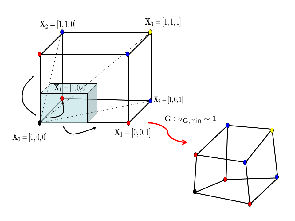
Figure 1: Figure illustrating the intuition behind our ML analysis for support recovery using binary $\mathbf{X}$ as an example. In the Figure $\mathbf{X}_{0}$ is the true signal that is taken to be the origin. Support error events with support errors more than $1$ are contained in union of events with support error of $1$ before the sensing/compression operator $\mathbf{G}$ is applied. This property is essentially preserved under the transformation by $\mathbf{G}$ if the minimum singular value of matrix $\mathbf{G}$ is well behaved.

The proof for the random Gaussian matrix $\mathbf{G}$ is based on the deterministic case. It turns out that the sparsity ratio $\alpha_{n}<0.04$ controls the singular values of the sub-matrix, namely, we can ensure $\sigma_{\mathbf{G},\min}>0$ with high probability for sparsity ratios below this number.

Note that we can also state these results in terms of sensing capacity. Formally, given any $\varepsilon>0$, there is an $n(\varepsilon)$ such that for all $n\geq n(\varepsilon)$ and any monotonic sequence $\alpha_{n}<0.04$, there are positive constants, $c_{1},\,c_{2}$, so

$$0<c_{1}\leq C_{n,\varepsilon}(\log(n),\alpha_{n},0)\leq c_{2}$$

In contrast to the optimistic results for output noise models, we have the following pessimistic result for the input noise model whose proof can be found in Section 3.1.1.

Theorem 3.3 (Input Noise Model:Necessity).

Consider the input noise model of Equation (2) with the signal set defined by Equation (4) and $\mathbf{G}$ drawn from an IID Gaussian ensemble with each component $g_{ij}\stackrel{{\scriptstyle d}}{{\sim}}{\cal N}(0,1/m)$. Let $\alpha_{n}$ be any positive monotonic sequence of sparsity ratios. Then recovery fails if $m=o\left({n\max(\log(n),\log({1\over\alpha_{n}}))\over\beta^{2}\textit{SNR}}\right)$. Alternatively, the sensing capacity is zero.

This says that for the input noise model one cannot expect meaningful compression in a noisy regime. To ensure support recovery either the SNR has to scale linearly with $n$, which implies essentially a noiseless regime, or the number of measurements must scale linearly with $n$ with any meaningful level of noise. This calls into question the sensor network motivated compression schemes such as those presented in [4] where the raw noisy measurements are randomly projected and transmitted to a fusion center.

3.0.1 Achievable Distortion Regions for Support Recovery

In this section we will describe results for approximate support recovery, namely, we allow some distortion in support recovery. An important implication of our result is that in the constant sparsity regime it is sufficient for SNR to be a constant independent of $n$ if we accommodate a constant fraction of support errors. We account for the support distortion as

$$d(\hat{\mathbf{X}},\mathbf{X}))=\frac{1}{k}\sum_{j=1}^{n}|I_{\{X_{i}\not=0\}}-I_{\{\hat{X}_{i}\not=0\}}|$$

where, $I_{\{\cdot\}}$ is the indicator function.

Theorem 3.4.

Consider the observation model of Equation (1) with $\mathbf{G}$ drawn from a Gaussian ensemble. Let $\mathbf{X}\in\Xi_{\beta}^{\{k\}}$ and let $d_{0}$ be as described above. It follows that if $\textit{SNR}\geq\frac{64H_{2}\left(\frac{2kd_{0}}{n}\right)}{\beta^{2}}$ and $m\geq 6nH_{2}\left(2\frac{k}{n}\right)$ the probability of support error greater than distortion $d_{0}$ goes to zero. Consequently, it follows that for support recovery with constant distortion, $d_{0}$, in the linear sparsity regime, i.e, $\alpha_{n}=k/n\geq\alpha>0$, it is sufficient for the SNR to be a constant independent of the signal dimension $n$.

Proof.

The proof is based on the proof of Theorem 3.2 and we refer the reader to the appendix. ∎

Note that Theorem 3.4 only trades off SNR with the distortion. However one would expect that with allowable distortion in support recovery it is possible to tradeoff number of measurements with distortion. In the following sections we will develop this tradeoff of number of measurements with the rate-distortion function by considering a Bayesian set-up. The main reason why this tradeoff is possible in a Bayesian set-up is due to the fact that before we analyzed a worst case set-up while in Bayesian case we analyze an average case scenario and it turns out that on an average the number of measurements can indeed be traded off with distortion.

3.1 Proof of Theorems 3.3 and 3.1: Necessary Conditions

We derive necessary conditions based on lower bounds to probability of error. As we pointed out in Equation (9) putting a suitable measure on the signal $\mathbf{X}$ can provide necessary conditions for the worst-case setup. This motivates employing different versions of Fano’s Lemma to establish the results. The standard version of the lemma appears in [18] and we repeat it here for the sake of completion:

Lemma 3.1.

Suppose ${\cal X}$ is a finite discrete set and $\mathbf{X}\in{\cal X}$ is distributed uniformly over this finite set. Let the observation $\mathbf{Y}$ be distributed according to the conditional distribution $\mathbb{P}(\mathbf{Y}|\mathbf{X})$, with $\mathbf{X}\in{\cal X}$. let $\hat{\mathbf{X}}(\mathbf{Y})$ denote the estimate of $\mathbf{X}$ given $\mathbf{Y}$. Then the probability of error in estimating $\mathbf{X}$ from $\mathbf{Y}$ is lower bounded by,

$$\mathbb{P}(\hat{\mathbf{X}}(\mathbf{Y})\neq\mathbf{X})\geq 1-\frac{\mathbb{I}(\mathbf{X};\mathbf{Y})+\log 2}{\log(|{\cal X}|-1)}$$

where $\mathbb{I}(\mathbf{X};\mathbf{Y})$ denotes the mutual information between $\mathbf{X}$ and $\mathbf{Y}$.

An alternate version of Fano’s lemma stated in [19] provides a lower bound for $N$-ary hypothesis testing.

Lemma 3.2.

Let $({\cal Y},{\cal B})$ be a $\sigma-$field and let $\mathbb{P}_{1},\ldots,\mathbb{P}_{N}$ be probability measures on ${\cal B}$ thought of as induced by $N$ hypotheses $\{1,\,2,\,\ldots,\,N\}$. Denote by $\theta(y)$ the estimator of the measures defined on ${\cal Y}$. Then

$$\max_{1\leq i\leq n}\mathbb{P}_{i}(\theta(y)\neq\mathbb{P}_{i})\geq\frac{1}{N}\sum_{i=1}^{N}\mathbb{P}_{i}(\theta(y)\neq\mathbb{P}_{i})\geq 1-\frac{\frac{1}{N^{2}}\sum_{i,j}D(\mathbb{P}_{i}\|\mathbb{P}_{j})+\log 2}{\log(N-1)}$$

where $\mathbb{P}_{i}$ means the distribution conditioned on the hypothesis $i$ and $D(\mathbb{P}_{i}\|\mathbb{P}_{j})$ is the Kullback-Liebler (KL) distance between the distributions $\mathbb{P}_{i}$ and $\mathbb{P}_{j}$.

Note that the use of these Lemmas requires a finite number of hypothesis or discrete alphabets. Therefore, in order to use these Lemmas for general $k$-sparse sequences $\mathbf{X}\in\Xi_{\beta}^{\{k\}}$ we first show that the worst case probability of error in support recovery is lower bounded by the probability of error in support recovery for $\mathbf{X}$ belonging to $k$-sparse sequences in $\left\{0,\beta\right\}^{n}$. To this end we have the following Lemma.

Lemma 3.3.

Let $\Xi_{\beta}^{\{k\}}$ be the family of $k$ sparse non-random sequences as defined in Equation (4). Denote the conditional distribution of $\mathbf{Y}$ given $\mathbf{X}$ as $\mathbb{P}(\mathbf{Y}\mid\mathbf{X})$. Let $\Xi_{\{0,\beta\}}^{\{k\}}=\{\mathbf{X}\in\Xi_{\beta}^{\{k\}}\mid X_{j}=\beta,\,\,j\in\mbox{Supp}(\mathbf{X})\}$ be a subset of $\Xi_{\beta}^{\{k\}}$ consisting of binary valued sequences. Let $\hat{\mathbf{X}}$ denote an estimator for $\mathbf{X}$ based on observation $\mathbf{Y}$. Then,

$$\mathbb{P}_{e|\mathbf{G}}=\min_{\hat{\mathbf{X}}\in\Xi_{\beta}^{\{k\}}}\max_{\mathbf{X}\in\Xi_{\beta}^{\{k\}}}\mathbb{P}\{\mbox{Supp}(\hat{\mathbf{X}})\neq\mbox{Supp}(\mathbf{X})|\mathbf{G},\mathbf{X}\} \geq\min_{\hat{\mathbf{X}}\in\Xi_{\beta}^{\{k\}}}\max_{\mathbf{X}\in\Xi_{\{0,\beta\}}^{\{k\}}}\mathbb{P}(\hat{\mathbf{X}}\neq\mathbf{X},\,\,\hat{\mathbf{X}}\in\Xi_{\{0,\beta\}}^{\{k\}}|\mathbf{G},\mathbf{X})$$

$$\geq \min_{\hat{\mathbf{X}}\in\Xi_{\{0,\beta\}}^{\{k\}}}\max_{\mathbf{X}\in\Xi_{\{0,\beta\}}^{\{k\}}}\mathbb{P}(\hat{\mathbf{X}}\neq\mathbf{X},\,\,\hat{\mathbf{X}}\in\Xi_{\{0,\beta\}}^{\{k\}}|\mathbf{G},\mathbf{X})$$ (10)

Proof.

See Appendix. ∎

The main idea behind the proofs of the results that follow below is to first lower bound the error probability by using Lemma 3.3 and restrict attention to binary sequences. Next we further restrict the signal class to a smaller subset of $\Xi_{\{0,\beta\}}^{\{k\}}$ of cardinality $n$. Then, finally using Lemma 3.2 we derive the lower bounds for the set of binary sequences. The lower bound thus obtained yields the necessary conditions.

3.1.1 Input Noise Model(Proof of Theorem 3.3)

From Lemma 3.3 it is sufficient to focus on the case when $\mathbf{X}$ belongs to the set of $k$-sparse sequences in $\left\{0,\beta\right\}^{n}$ and any subset of these sequences. We will establish the first part of the Theorem as follows:- Let $\Xi_{\{0,\beta\}}^{\{\eta\}}$ be the subset of $\eta<k$ sparse binary valued sequences. Let $\mathbf{X}_{0}\in\Xi_{\{0,\beta\}}^{\{\eta\}}$, be an arbitrary element with support $\mbox{Supp}(\mathbf{X}_{0})=\eta-1$. Next choose $n$ elements $\mathbf{X}_{j},\,j=1,\,2,\,\ldots,\,n$ with support equal to $\eta$ and at a unit Hamming distance from $\mathbf{X}_{0}$. Denote by the probability kernel $\mathbb{P}_{j},\,0\leq j\leq n$ the induced observed distributions. Under the AWGN noise model, for a given $\mathbf{G}$, and a fixed set of elements, $\mathbf{X}_{j}$, the probability kernels are Gaussian distributed, i.e.,

$${\cal H}_{j}:\mathbf{Y}\stackrel{{\scriptstyle d}}{{\sim}}\mathbb{P}_{j}\equiv{\cal N}\left(\mathbf{G}\mathbf{X}_{j},\frac{\mathbf{\Sigma}}{{\textit{SNR}}}\right),\,\,j=0,\,1,\,\ldots,\,n$$

where $\mathbf{\Sigma}=\mathbf{G}\mathbf{G}^{T}$. Furthermore we have $n+1$ hypotheses. Consider now the support recovery problem. It is clear that the error probability can be mapped into a corresponding hypothesis testing problem. For this we consider $\theta(\mathbf{Y})$ as estimate of one of the $n+1$ distributions above and we have the following set of inequalities.

$$\mathbb{P}_{e\mid\mathbf{G}}=\max_{\mathbf{X}\in\Gamma^{\eta}}\mathbb{P}_{\mathbf{X}}(\hat{\mathbf{X}}\neq\mathbf{X}\mid\mathbf{G})=\max_{j}\mathbb{P}_{j}(\theta(\mathbf{Y})\neq\mathbb{P}_{j}\mid\mathbf{G})\geq\frac{1}{n+1}\sum_{j=0}^{n}\mathbb{P}_{j}(\theta(\mathbf{Y})\neq\mathbb{P}_{j}\mid\mathbf{G})$$

where we write $\mathbb{P}_{e\mid\mathbf{G}}$ to point out that the probability of error is conditioned on $\mathbf{G}$. Applying Lemma 3.2 it follows that the probability of error in exact support recovery is lower bounded by,

$$\mathbb{P}_{e\mid\mathbf{G}}\geq\frac{\log(n)-\frac{1}{(n+1)^{2}}\sum_{i,j,i\neq j}D(\mathbb{P}_{i}\|\mathbb{P}_{j})-\log 2}{\log(n)}$$

We observe that under AWGN noise $\mathbf{N}$ that,

$$D(\mathbb{P}_{i}\|\mathbb{P}_{j})=\textit{SNR}(\mathbf{X}_{i}-\mathbf{X}_{j})^{T}\mathbf{G}^{T}\mathbf{\Sigma}^{-1}\mathbf{G}(\mathbf{X}_{i}-\mathbf{X}_{j})=\textit{SNR}(\mathbf{X}_{i}-\mathbf{X}_{j})^{T}\mathbf{V}\left[\begin{array}[]{cc}I&0\\ 0&0\end{array}\right]\mathbf{V}^{*}(\mathbf{X}_{i}-\mathbf{X}_{j})$$ (13)

where $\mathbf{\Sigma}=\mathbf{G}\mathbf{G}^{T}$, $\mathbf{G}=\mathbf{U}[\mathbf{\Lambda},\,\,0]\mathbf{V}^{*}$ is the SVD of $\mathbf{G}$ with $\mathbf{V}=[\mathbf{v}_{1},\mathbf{v}_{2},\,\mathbf{v}_{3},\,\ldots,\,\mathbf{v}_{n}]=[v_{rs}]$. The last equality in Equation (13) follows from straightforward algebraic manipulations. Now by noting that $(\mathbf{X}_{i}-\mathbf{X}_{j})$ is at most a 2-sparse vector with its non-zero entries equal to $\beta$ at some locations $q$ and $p$, we can further reduce the last expression to $D(\mathbb{P}_{i}\|\mathbb{P}_{j})=\textit{SNR}\beta^{2}\sum_{l=1}^{m}(v_{pl}-v_{ql})^{2}$. Now using the standard rotational invariance properties of IID Gaussian matrices  [20], that its singular vectors are uniformly distributed over a sphere, it follows by taking expectations and using symmetry that,

$$\mathbb{P}_{e}=\mathbf{E}_{\mathbf{G}}\mathbb{P}_{e\mid\mathbf{G}}\geq\frac{\log(n)-\frac{n}{n+1}\frac{2\beta^{2}\textit{SNR}\,m}{n}-\log 2}{\log(n)}$$ (14)

Now, the error probability is bounded away from zero by $\epsilon$ if the number of measurements scales as follows:

$$m=o\left({(n+1)\log(n)\over\beta^{2}\textit{SNR}}\right)$$

To establish the second upper bound we consider the family, $\Xi_{\{0,\beta\}}^{k}$ of exact k-sparse binary valued sequences which form a subset of $\Xi_{\{0,\beta\}}^{\{k\}}$. Following similar logic as in the proof of the first part, for the set of exactly $k$-sparse sequences, we form the corresponding $\binom{n}{k}$ hypotheses. Then,

$$\mathbb{P}_{e}=\mathbf{E}_{\mathbf{G}}\mathbb{P}_{e\mid\mathbf{G}}\geq\frac{\log(\binom{n}{k}-1)-\frac{1}{\binom{n}{k}^{2}}\sum_{i,j,i\neq j}D(\mathbb{P}_{i}\|\mathbb{P}_{j})-\log 2}{\log(\binom{n}{k}-1)}$$ (15)

We compute the average pairwise KL distance,

$$\frac{1}{{n\choose k}^{2}}\sum_{i,j,i\neq j}D(\mathbb{P}_{i}\|\mathbb{P}_{j})$$

$$=\frac{1}{{n\choose k}}\sum_{j=1}^{k}\textit{SNR}(\mathbf{X}-\mathbf{X}^{\prime})^{T}\mathbf{G}^{T}\mathbf{\Sigma}^{-1}\mathbf{G}(\mathbf{X}-\mathbf{X}^{\prime}).\sharp(\mbox{sequences $\mathbf{X}^{\prime}$ at hamming distance 2j from $\mathbf{X}$})$$

The equality above follows from symmetry. Again using the standard rotational invariance properties of IID Gaussian matrices [20], the above equation implies that ,

$$\frac{1}{{n\choose k}^{2}}\sum_{i,j,i\neq j}D(\mathbb{P}_{i}\|\mathbb{P}_{j})=\frac{m}{n}\frac{1}{{n\choose k}}\sum_{j=1}^{k}\textit{SNR}\beta^{2}{n-k\choose j}{k\choose j}(2j)=\frac{m}{n}2\beta^{2}\textit{SNR}\alpha_{n}n(1-\alpha_{n})$$

where the last equality follows from standard combinatorial identity. The proof then follows by noting that for large enough value of $n$, $\log(\binom{n}{k}-1)\geq\alpha_{n}n\log\frac{1}{\alpha_{n}}$.

3.1.2 Output Noise Model (Proof of Theorem 3.1)

We will now establish Theorem 3.1 namely, that if $SNR=o(\log(n))$ support recovery is impossible. Furthermore, if $SNR=O(\log(n))$ support recovery will be impossible if the number of measurements scales as $o(k\log(n/k))$. The first part follows from the following Proposition.

Proposition 3.1 (Output noise model - SNR Bound).

For the observation model of Equation (1) with the signal set of Equation (4) the SNR must scale with $\frac{\log(n)}{2\beta^{2}}$ for perfect support recovery irrespective of which sensing matrix is used.

Proof.

The proof follows along the same lines as the proof of Theorem 3.3 with $\mathbf{\Sigma}=\mathbf{I}$ up to Equation (13). In the Kullback Leibler distance calculation we are now left with the term $\mathbf{G}^{T}\mathbf{G}$. Since $\mathbf{G}$ is normalized its expected value is identity. Therefore, we no longer get the factor $n/m$ in Equation 14. Consequently, following the rest of the steps we have that, $2\beta^{2}\textit{SNR}\geq\log(n)$ for exact support recovery. ∎

Next we establish what happens for $SNR=O(\log(n))$ to prove the second part of Theorem 3.1. First, note that if the sparsity, $k$, grows linearly with the signal dimension, $n$, there is nothing to prove, since it is well-known [1] that the number of measurements must scale at least as $2k+1=\Omega(n)$ even when there is no noise to guarantee support recovery. For this reason we focus on the sub-linear case namely, $k=n^{-\gamma},\,\,\gamma<1$. We consider the subset $\Xi_{\{0,\beta\}}^{k}$ consisting of strictly $k$-sparse sequences taking values in $\{0,\beta\}^{n}$. From Lemma 3.3 we see that it is sufficient to focus on this set. Applying Lemma 3.1 with a uniform prior on the support set we get

$$\max_{\mathbf{X}\in{\cal X}}\mathbb{P}(\hat{\mathbf{X}}\neq\mathbf{X}|\mathbf{X},\mathbf{G})\geq\mathbb{P}(\hat{\mathbf{X}}\neq\mathbf{X}|\mathbf{G})\geq 1-\frac{\mathbb{I}(\mathbf{X};\mathbf{Y}|\mathbf{G})+\log 2}{\log(|{\cal X}|-1)}$$ (16)

where ${\cal X}=\Xi_{\{0,\beta\}}^{k}\subset\{0,\beta\}^{n}$ is the discrete alphabet in which values of $\mathbf{X}$ are realized. The first inequality follows because the worst-case probability of error is larger than the Bayesian error.

Note that strictly speaking since we are interested in the support errors, the probability of error events and the mutual information term must contain the support of $\mathbf{X}$ as the variable but since we are restricting ourselves to binary valued sequences $\mathbf{X}\in\Xi_{\{0,\beta\}}^{k}$, knowing the support implies that we know $\mathbf{X}$.

Now $\log|{\cal X}|=\log\binom{n}{k}$ since there are $\binom{n}{k}$ such hypothesis consisting of all the possible support locations with cardinality $k$. We will now upper bound the mutual information term. It follows that,

$$\mathbb{I}(\mathbf{X};\mathbf{Y}|\mathbf{G}) =h(\mathbf{Y}|\mathbf{G})-h(\mathbf{Y}|\mathbf{X},\mathbf{G})\leq h(\mathbf{Y})-h(\mathbf{N})\stackrel{{\scriptstyle(a)}}{{\leq}}\sum_{i=1}^{m}h(Y_{i})-\frac{m}{2}\log\left(2\pi e\frac{1}{SNR}\right)$$

$$\stackrel{{\scriptstyle(b)}}{{\leq}}\frac{m}{2}\log\left(2\pi e\left(\frac{k\beta^{2}}{m}+\frac{1}{SNR}\right)\right)-\frac{m}{2}\log(2\pi e\frac{1}{SNR})=\frac{m}{2}\log(1+\frac{k\beta^{2}\textit{SNR}}{m})$$

where $h(\cdot)$ is the differential entropy; (a) follows from the fact that the noise is Gaussian and the chain rule together with the fact that conditioning reduces entropy; (b) follows from the fact that Gaussian distributions maximizes differential entropy. Now from Equation (16) it follows that the number of measurements must satisfy,

$$m\geq\dfrac{\log\left(\binom{n}{k}-1\right)}{\log(1+\frac{k\beta^{2}\textit{SNR}}{m})+\frac{\log 2}{m}}$$ (17)

Next unless $\textit{SNR}=\Omega(\log(n))$ we know from Proposition 3.1 that support recovery is impossible. Hence we set $\textit{SNR}=\log(n)$, which is the minimum possible. We next establish the theorem by contradiction. To this end let the number of measurements scale as $m=\rho_{n}\log(\binom{n}{k})$, with $\rho_{n}\rightarrow 0$, then, by rearranging the terms in Equation (17) we get

$$\log\left(1+\frac{k\beta^{2}\textit{SNR}}{\rho_{n}\log(\binom{n}{k})}\right)+\frac{\log 2}{\rho_{n}\log(\binom{n}{k})}\geq\dfrac{\log\left(\binom{n}{k}-1\right)}{\rho_{n}\log(\binom{n}{k})}$$ (18)

Next note that the expression on the left can be simplified by noting that

$$\frac{k\beta^{2}\textit{SNR}}{\rho_{n}\log(\binom{n}{k})}=\Theta\left({1\over\rho_{n}(1-{\log(k)\over\log(n)})}\right)$$

while the expression on the right has the scaling $\Theta(\rho_{n}^{-1})$. Consequently, if maximum admissible sparsity, $k$, grows sub-linearly with $n$ then $\log(1+\frac{k\beta^{2}\textit{SNR}}{\rho_{n}\log(\binom{n}{k})})=\Theta(\log(1+\rho_{n}^{-1}))$ and Equation (18) can never be satisfied since $\rho_{n}\rightarrow 0$. This shows that for sub-linear cases recovery is impossible if $m=o(\log(\binom{n}{k}))=o(nH_{2}(\alpha_{n}))$.

Remark 3.2.

Note that unless SNR scales as $n^{\delta}$ for some $\delta>0$ we will still need the measurements to scale as $\Omega(k\log(n/k))$ to guarantee support recovery.

3.2 Proof of Theorem 3.2: Deterministic Case

In this section we derive sufficient conditions for support recovery for the output noise model for any given arbitrary deterministic matrix $\mathbf{G}$ and for general noise covariance $\mathbf{\Sigma}$. For the output noise model of Equation (1), we assume that each column of the deterministic $\mathbf{G}$ is normalized. Subsequently we specialize these results to the case when $\mathbf{G}$ is chosen from the Gaussian ensemble and with $\mathbf{\Sigma}=\mathbf{I}$.

To simplify the exposition we introduce several new variables. We associate each admissible signal, $\mathbf{X}\in\Xi^{\{k\}}$ by its support, $S$. We denote by $\mathbf{X}_{S}$ the signal, $\mathbf{X}$, restricted to the set of components indexed by $S$. Similarly, we denote by $\mathbf{G}_{S}$ the matrix formed from columns indexed by $S$. Since the maximum sparsity level is $k$ the number of different support sets is equal to $\sum_{j=1}^{k}{n\choose j}-1$. We index the different support sets as $S_{\omega}$ with $\omega\in{\cal I}=\left\{0,\,1,\,2,\,\ldots,\sum_{j=1}^{k}{n\choose j}-1\right\}$. Also we denote by $\mathbf{X}_{S_{\omega}}^{\min}$ the minimum absolute value of the components of the signal $\mathbf{X}$ on the support set $S_{\omega}$, i.e., $\mathbf{X}_{S_{\omega}}^{\min}=\min\{|X_{j}|:j\in S_{\omega}\}$. Without loss of generality we assume that the true signal is $\mathbf{X}_{0}$, the support set of the true signal to be $S_{0}$ corresponding to $\omega=0$. We denote by $X_{0,j}$ the jth component of the true signal.

For any $\omega\not=0$, we denote the overlapping support by, $S_{0,\omega}$, false detection by, $S_{0^{c},\omega}$ and missed detection by, $S_{0,\omega^{c}}$, namely,

$$\mbox{Overlap}- S_{0,\omega}=S_{0}\cap S_{\omega}$$

$$\mbox{False Alarms}- S_{0^{c},\omega}=S_{0}^{c}\cap S_{{\omega}}$$

$$\mbox{Misses}- S_{0,\omega^{c}}=S_{0}\cap S_{\omega}^{c}$$

For a given noise covariance $\mathbf{\Sigma}$ the ML estimator is given by,

$$\hat{\mathbf{X}}=\min_{\mathbf{X}\in\Xi_{\beta}^{\{k\}}}(\mathbf{Y}-\mathbf{G}\mathbf{X})^{T}\mathbf{\Sigma}^{-1}(\mathbf{Y}-\mathbf{G}\mathbf{X})$$

The above ML estimator is hard to analyze. In order to simplify the analysis we will consider a sub-optimal ML estimator. To this end consider the set, $\Xi_{\beta/2}^{\{k\}}$. Clearly, $\Xi_{\beta}^{\{k\}}\subset\Xi_{\beta/2}^{\{k\}}$. We propose the following sub-optimal ML estimator,

$$\hat{\mathbf{X}}=\arg\min_{\mathbf{X}\in\Xi_{\beta/2}^{\{k\}}}\|\mathbf{Y}-\mathbf{G}\mathbf{X}\|^{2}$$ (19)

and report $\mbox{Supp}(\hat{\mathbf{X}})$ as the final solution. Note that this estimator is sub-optimal since it is prone to more errors. To see this note that we consider a larger signal set and we ignore possible noise correlation $\mathbf{\Sigma}$ in our estimator. Consequently, the error probability in detecting the correct support can only be larger than the optimal ML estimator. The performance of the relaxed estimator provides an upper bound for the performance of ML estimator. Hence, we can write,

$$\mathbb{P}^{ML}_{e\mid\mathbf{G}}\leq\mathbb{P}_{e\mid\mathbf{G}}=\mathbb{P}\left(\mathbf{N}:\min_{\omega\not=0,\,\mathbf{X}_{S_{\omega}}^{\min}\geq\beta/2}\|\mathbf{Y}-\mathbf{G}_{S_{\omega}}\mathbf{X}_{S_{\omega}}\|^{2}\leq\min_{\mathbf{X}_{S_{0}}^{\min}\geq\beta/2}\|\mathbf{Y}-\mathbf{G}_{S_{0}}\mathbf{X}_{S_{0}}\|^{2}\right)$$ (20)

Note that in the above expression $\mathbf{X}_{S_{0}}$ is not the true signal, $\mathbf{X}_{0}$, but any other signal whose support is identical to that of the true signal. We then have the following result.

Lemma 3.4.

$$\mathbb{P}^{ML}_{e\mid\mathbf{G}}\leq\mathbb{P}_{e\mid\mathbf{G}}\leq\mathbb{P}({\cal E}_{1})+\mathbb{P}({\cal E}_{2})$$

where

$${\cal E}_{1}=\{\mathbf{N}:\min_{\omega\not=0,\,\mathbf{X}_{S_{\omega}}^{\min}\geq\beta/2}\|\mathbf{Y}-\mathbf{G}_{S_{\omega}}\mathbf{X}_{S_{\omega}}\|^{2}\leq\min_{\tilde{\mathbf{X}}}\|\mathbf{Y}-\mathbf{G}_{S_{0}}\tilde{\mathbf{X}}\|^{2}\}$$

$${\cal E}_{2}=\left\{\mathbf{N}:\|(\mathbf{G}_{S_{0}}^{T}\mathbf{G}_{S_{0}})^{-1}\mathbf{G}_{S_{0}}^{T}\mathbf{N}\|_{\infty}\geq\beta/2\right\}$$

Proof.

First note the following qualitative points. In the event ${\cal E}_{1}$ we have replaced the constrained minimization on the R.H.S. of the inequality in the error event with an unconstrained one. This will simplify the subsequent analysis as closed form expressions can be obtained. The event ${\cal E}_{2}$ captures the probability that the unconstrained minimization in ${\cal E}_{1}$ is very far from the constrained one. Here we use the fact that the minimum component on the support of the true signal $\mathbf{X}_{0}$ is greater than $\beta$. We also relax our ML estimator so that we find a best fit with any signal sharing the same support set, $S_{0}$, as $\mathbf{X}_{0}$ but with $\mathbf{X}_{S_{0}}^{\min}\geq\beta/2$. Now, denote

$$A\overset{\Delta}{=}\left\{\mathbf{N}:\min_{\omega\not=0,\,\mathbf{X}_{S_{\omega}}^{\min}\geq\beta/2}\|\mathbf{Y}-\mathbf{G}_{S_{\omega}}\mathbf{X}_{S_{\omega}}\|^{2}\leq\min_{\mathbf{X}_{S_{0}}^{\min}\geq\beta/2}\|\mathbf{Y}-\mathbf{G}_{S_{0}}\mathbf{X}_{S_{0}}\|^{2}\right\}$$

$$B\overset{\Delta}{=}\left\{\mathbf{N}:\min_{\mathbf{X}_{S_{0}}^{\min}\geq\beta/2}\|\mathbf{Y}-\mathbf{G}_{S_{0}}\mathbf{X}_{S_{0}}\|^{2}=\min_{\tilde{\mathbf{X}}}\|\mathbf{Y}-\mathbf{G}_{S_{0}}\tilde{\mathbf{X}}\|^{2}\right\}$$

Then we have

$$\mathbb{P}_{e}=\mathbb{P}(A)=\mathbb{P}(A\cap B)+\mathbb{P}(A\cap\bar{B})\leq\mathbb{P}(A\cap B)+\mathbb{P}(\bar{B})$$

The Lemma then follows by noting that,

$$A\cap B = \left\{\mathbf{N}:\min_{\mathbf{X}_{S_{\omega}}^{\min}\geq\beta/2,\omega\neq 0}\|\mathbf{Y}-\mathbf{G}_{S_{\omega}}\mathbf{X}_{S_{\omega}}\|^{2}\leq\min_{\mathbf{X}_{S_{0}}^{\min}\geq\beta/2}\|\mathbf{Y}-\mathbf{G}_{S_{0}}\mathbf{X}_{S_{0}}\|^{2}\right\}\cap B$$

$$= \left\{\mathbf{N}:\min_{\mathbf{X}_{S_{\omega}}^{\min}\geq\beta/2,\omega\neq 0}\|\mathbf{Y}-\mathbf{G}_{S_{\omega}}\mathbf{X}_{S_{\omega}}\|^{2}\leq\min_{\tilde{\mathbf{X}}}\|\mathbf{Y}-\mathbf{G}_{S_{0}}\tilde{\mathbf{X}}\|^{2}\right\}={\cal E}_{1}$$

and,

$$\bar{B}=\left\{\mathbf{N}:\min_{\mathbf{X}_{S_{0}}^{\min}\geq\beta/2}\|\mathbf{Y}-\mathbf{G}_{S_{0}}\mathbf{X}_{S_{0}}\|^{2}\not=\min_{\tilde{\mathbf{X}}}\|\mathbf{Y}-\mathbf{G}_{S_{0}}\tilde{\mathbf{X}}\|^{2}\right\}\subset{\cal E}_{2}$$

∎

From the above Lemma, it is sufficient to focus on events ${\cal E}_{1}$ and ${\cal E}_{2}$ separately. The following lemma provides a result that considerably simplifies the error event ${\cal E}_{1}$. It turns out that the event ${\cal E}_{1}$ is a subset of the union of atomic events, namely,

Lemma 3.5.

For $m\geq 2k+1$,

$${\cal E}_{1}\subseteq\tilde{\cal E}_{1}=\bigcup_{X\in\{\beta/2,-\beta/2\}}\bigcup_{j=1}^{n}\left\{\mathbf{N}:2\mathbf{N}^{T}\mathbf{g}_{j}X\geq\sigma_{\mathbf{G},\min}|X|^{2}\right\}$$

where, $\mathbf{g}_{j}$ is the $j-th$ column of the matrix $\mathbf{G}$ and

$$\sigma_{\mathbf{G},\min}=\min_{|S|\leq 2k}\sigma_{\min}(\mathbf{G}_{S}^{T}\mathbf{G}_{S})$$ (21)

where $\sigma_{\min}(\mathbf{G}_{S}^{T}\mathbf{G}_{S})$ denotes the minimum singular values of $\mathbf{G}_{S}^{T}\mathbf{G}_{S}$.

Proof.

See Appendix. ∎

We now have the following Lemma.

Lemma 3.6.

Consider the output noise model for a deterministic matrix $\mathbf{G}$ with $m\geq 2k+1$ and $\mathbf{N}$ distributed as ${\cal N}(0,\mathbf{\Sigma})$. The probability of the error event ${\cal E}_{1}$ is upper bounded by,

$$\mathbb{P}({\cal E}_{1})\leq\exp\left\{-\sigma_{\mathbf{G},\min}^{2}\frac{\lambda_{min}(\mathbf{\Sigma}^{-1})\beta^{2}\textit{SNR}}{32}\right\}\exp\{\log 2n\}$$ (22)

where $\lambda_{\min}(\mathbf{\Sigma}^{-1})$ is the minimum eigenvalue value of the matrix $\mathbf{\Sigma}^{-1}$.

Proof.

See Appendix. ∎

We now have the following Lemma for the error event ${\cal E}_{2}$. Again note that the result applies to any matrix $\mathbf{G}$ (not necessarily Gaussian).

Lemma 3.7.

For the setup of Lemma 3.6, we have,

$$\mathbb{P}({\cal E}_{2})\leq\exp\left\{-\sigma_{\mathbf{G},\min}^{2}\frac{\lambda_{\min}(\mathbf{\Sigma}^{-1})\beta^{2}\textit{SNR}}{8}+\log 2n\right\}$$

Proof.

See Appendix. ∎

By combining Lemmas 3.6 and 3.7 we can prove the deterministic case of Theorem 3.2. We state it as a proposition since we will refer to it later.

Proposition 3.2.

Consider the setup of Lemma 3.6. Then for exact support recovery it is sufficient that $m\geq 2k+1$ and $\textit{SNR}=\Omega\left(\dfrac{1}{\sigma_{\mathbf{G},\min}^{2}}\dfrac{64\log 2n}{\beta^{2}\lambda_{\min}(\mathbf{\Sigma}^{-1})}\right)$.

Proof.

From Lemmas 3.6 and 3.7 it follows that for $m\geq 2k+1$,

$$\mathbb{P}_{e|\mathbf{G}} \leq\exp\left\{-\sigma_{\mathbf{G},\min}^{2}\frac{\lambda_{\min}(\mathbf{\Sigma}^{-1})\beta^{2}\textit{SNR}}{32}+\log 2n\right\}+\exp\left\{-\sigma_{\mathbf{G},\min}^{2}\frac{\lambda_{\min}(\mathbf{\Sigma}^{-1})\beta^{2}\textit{SNR}}{8}+\log 2n\right\}$$

$$\leq 2\exp\left\{-\sigma_{\mathbf{G},\min}^{2}\frac{\lambda_{\min}(\mathbf{\Sigma}^{-1})\beta^{2}\textit{SNR}}{32}+\log 2n\right\}$$

Therefore for $\textit{SNR}=2\cdot\sigma_{\mathbf{G},\min}^{-2}\dfrac{32\log 2n}{\beta^{2}\lambda_{\min}(\mathbf{\Sigma}^{-1})}$ the probability of error $\mathbb{P}_{e|\mathbf{G}}\leq 2e^{-\log 2n}$. Thus with $n\rightarrow\infty$, $\mathbb{P}_{e|\mathbf{G}}$ goes to zero as $\frac{1}{n}$. This implies that SNR scaling of $\Omega\left(\sigma_{\mathbf{G},\min}^{-2}\dfrac{64\log 2n}{\beta^{2}\lambda_{\min}(\mathbf{\Sigma}^{-1})}\right)$ is sufficient. ∎

3.3 Proof of Theorem 3.2: Gaussian Case

We will now focus on sensing matrices, $\mathbf{G}$, drawn from an IID Gaussian ensemble. As in the deterministic case we need to bound the probabilities of events, ${\cal E}_{1}$ and ${\cal E}_{2}$. We will first focus our attention on event ${\cal E}_{1}$.

We point out that the proof for the deterministic case cannot be directly applied. First, note that $\sigma_{\mathbf{G},\min}$ of Equation (21) is now a random variable. Therefore, we need to average over this random variable in computing an upperbound to the probability of events ${\cal E}_{1},\,{\cal E}_{2}$. A second problem is that in the deterministic case we assumed that the $\ell_{2}$ norm of each column, $\mathbf{g}_{j}$ is deterministically normalized to unity. In the Gaussian case only the expected power is normalized to unity. Note also that for the output noise model considered in this paper $\mathbf{\Sigma}=\mathbf{I}$. Therefore $\lambda_{\min}(\mathbf{\Sigma}^{-1})=1$. Following along the lines of the proof of Lemma 3.6 we see that,

$$\mathbb{P}({\cal E}_{1}\mid\mathbf{G})\leq\exp\left\{-\frac{\sigma_{\mathbf{G},\min}^{2}\beta^{2}\textit{SNR}}{32\max_{j}\|\mathbf{g}_{j}\|_{2}}\right\}\exp\{\log 2n\}$$

We need to now characterize a lower bound for ${\sigma_{\mathbf{G},\min}^{2}\over\max_{j}\|\mathbf{g}_{j}\|_{2}}$. To this end we observe that,

$$\Pr\left({\sigma_{G,\min}^{2}\over\max_{j}\|\mathbf{g}_{j}\|_{2}}\geq{(1-\eta)^{2}\over 1+\epsilon}\right)\geq\Pr(\sigma_{G,\min}\geq (1-\eta)^{2},\,\max_{j}\|\mathbf{g}_{j}\|_{2}\leq 1+\epsilon)$$ (23)

$$\geq 1-(\Pr(\sigma_{G,\min}\leq(1-\eta)^{2})+\Pr(\max_{j}\|\mathbf{g}_{j}\|_{2}\geq 1+\epsilon))$$

This implies that we should characterize $\sigma_{G,\min}$ and $\max_{j}\|\mathbf{g}_{j}\|_{2}$ separately. We appeal to the following lemma in [2], to characterize $\sigma_{G,\min}$.

Lemma 3.8.

Suppose the sparsity is $\alpha_{n}=k/n$ and we consider a function $f(q):=\sqrt{n/m}\left(\sqrt{q}+\sqrt{2H_{2}(q)}\right)$, where $H_{2}(q):=-q\log q-(1-q)\log(1-q)$. Let $\mathbf{G}$ be an $m\times n$ matrix drawn from a Gaussian ensemble with $g_{ij}\stackrel{{\scriptstyle d}}{{\sim}}{\cal N}(0,1/m)$. Then it follows that $\sigma_{\mathbf{G},\min}$ described in Equation 21 has the following concentration property,

$$\mathbb{P}\left(\sigma_{\mathbf{G},\min}\leq 1-\eta\right)\leq 2\exp\left(-{n\epsilon H_{2}(\alpha_{n})\over 2}\right)\stackrel{{\scriptstyle\Delta}}{{=}}\delta_{1}(n,\alpha_{n},\epsilon)$$ (24)

where, $\eta=2(1+\varepsilon)f(2\alpha)+(1+\varepsilon)^{2}f^{2}(2\alpha)$.

We consider the following concentration result to characterize maximum power of the columns of $\mathbf{G}$.

Lemma 3.9.

Let $\mathbf{G}$ be drawn from an IID Gaussian ensemble with $g_{ij}\stackrel{{\scriptstyle d}}{{\sim}}{\cal N}(0,1/m)$. Let $\mathbf{g}_{j},\,j=1,\,2\,\ldots,\,n$ be the columns of $\mathbf{G}$. Then, for any $\epsilon>0$, it follows that,

$$\mathbb{P}(\max_{j}\|\mathbf{g}_{j}\|^{2}_{2}\geq 1+\epsilon)\leq\exp\left(-{m\over 2}(\log(1+\epsilon)+\epsilon)+\log n\right)\stackrel{{\scriptstyle\Delta}}{{=}}\delta_{2}(m,n,\epsilon)$$

Proof.

Clearly $X:=m\|\mathbf{g}\|^{2}_{2}$ is $\chi^{2}$ distributed with degree $m$ and its moment generating function is $\mathbb{E}(e^{tX})=(1-2t)^{-m/2}$. From Chernoff bound,

$$\Pr(X\geq a)\leq\frac{\mathbb{E}(e^{tX})}{e^{ta}}=\frac{(1-2t)^{-m/2}}{e^{ta}}$$

Choosing $a=m(1+\epsilon)$ and $t=\frac{1}{2}(1-m/a)=\frac{\epsilon}{2(1+\epsilon)}$, we have

$$\Pr(\|\mathbf{g}\|^{2}_{2}\geq 1+\epsilon)\leq\exp\left(-{m\over 2}(\log(1+\epsilon)+\epsilon)\right)$$

The proof then follows by employing the union bound. ∎

Putting Lemmas 3.8 and 3.9 together with Equation (23) and taking the expectation with respect to $\mathbf{G}$ we get,

$$\mathbb{P}({\cal E}_{1})= E_{\mathbf{G}}\left(\mathbb{P}({\cal E}_{1}\mid\mathbf{G})I_{\Gamma}+\mathbb{P}({\cal E}_{1}\mid\mathbf{G})I_{\Gamma^{c}}\right)$$

$$\leq\exp\left\{-\frac{(1-\eta)^{2}\beta^{2}\textit{SNR}}{32(1+\varepsilon)}\right\}\exp\{\log 2n\}(1-\delta)+\delta$$

where $\Gamma=\{\mathbf{G}:{\sigma_{\mathbf{G},\min}\over\max_{j}\|\mathbf{g}_{j}\|_{2}}\leq{(1-\eta)^{2}\over(1+\varepsilon)}\}$ and $\delta=\delta_{1}(n,\alpha_{n},\epsilon)+\delta_{2}(m,n,\epsilon)$. Note that $\mathbb{P}(\Gamma^{c})\leq\delta$ and $\delta$ can be made arbitrarily small for $m=\Omega(\log(n))$ and $k$ sufficiently large. We are now left to ensure that the first term in the RHS of the above equation can be made small as well. For this purpose we need

$$\frac{(1-\eta)^{2}\beta^{2}\textit{SNR}}{(1+\epsilon)32}=(1+\gamma)\log 2n$$ (25)

for some arbitrary $\gamma>0$. Let $\eta_{1}=\left(\frac{32(1+\gamma)(1+\epsilon)\log 2n}{\beta^{2}\textit{SNR}}\right)^{1/2}$. This implies that it is sufficient that,

$$1-\eta\geq\eta_{1}\implies\eta\leq 1-\eta_{1}$$ (26)

$$\implies(1+\varepsilon)f(2\alpha)(2+(1+\varepsilon)f(2\alpha))+1\leq 1+(1-\eta_{1})$$ (27)

$$\implies(1+(1+\varepsilon)f(2\alpha))^{2}\leq 2-\eta_{1}\implies(1+\varepsilon)f(2\alpha)\leq\sqrt{2-\eta_{1}}-1$$ (28)

For this inequality to be satisfied we need $\eta_{1}\leq 1$. A sufficient condition for support recovery can be obtained by substituting for $\eta$ and we get

$$\eta_{1}={32(1+\gamma)(1+\epsilon)\log(2n)\over\beta^{2}\textit{SNR}}<1,\,\,{n\over m}\leq\frac{1}{(1+\varepsilon)^{2}(\sqrt{2\alpha}+\sqrt{2H_{2}(2\alpha)})^{2}}(\sqrt{2-\eta_{1}}-1)^{2}$$

Since $(\sqrt{2\alpha}+\sqrt{2H_{2}(2\alpha)})^{2}\leq 6H_{2}(2\alpha)$ and $\gamma,\,\varepsilon$ can be made arbitrarily small, the result now follows for event ${\cal E}_{1}$.

We are now left to bound the probability of event ${\cal E}_{2}$. This case is simple since the normalizing factor $\max_{j}\|\mathbf{g}_{j}\|_{2}$ is no longer relevant as seen from the proof of Lemma 3.7. It suffices to ensure that $\sigma_{\mathbf{G},\min}$ needs to be bounded away from zero. However, note that we already have this from bounding the probability of event ${\cal E}_{1}$. The result now follows.

4 Recovery for Arbitrary Distortions: Bayesian signal model

In this section we switch to a Bayesian signal model from the worst-case setting considered in the previous section. There are a number of reasons for considering such a model:
(A) For both the input and output noise models we need the SNR to scale as $\Omega(\log(n))$ for exact support recovery regardless of the number of measurements.
(B) For exact support recovery in the worst-case setup we require that the minimum singular values of all sub-matrices of $\mathbf{G}$ as described in Equation (21) be uniformly bounded away from zero (Theorem 3.2). This arises because a worst-case signal, $\mathbf{X}$, matched to the smallest singular value can be chosen. However, this problem may not arise in the average case setting.
(C) The situation is worse for the input noise model. Even with SNR of $\Omega(\log(n))$ the number of measurements required is linearly proportional to signal dimension.
(D) Theorem 3.4 points out that even with distortion we can only hope to reduce the SNR but not the number of measurements.

Consequently, it is worth exploring whether these results can be improved in the average Bayesian case. Fundamentally, the idea is that if we remove a sufficiently small set of signals then it is conceivable that the results could be more promising.

In the following we first develop novel lower and upper bounds to probability of error subject to a distortion in reconstruction. The main ingredient in realizing these bounds is the use of the minimal covering property of the rate distortion function. We begin with a minimal cover as a functional mapping of the source to the set of rate distortion quantization points. Then for the lower bound to the probability of error we follow the steps of the proof Fano’s inequality, [18] which we appropriately modify to address detection of the correct quantization point corresponding to the true $\mathbf{X}$. Similarly for the upper bound to the probability of error we propose a minimum distance decoder (ML decoder for AWGN noise) over the set of rate distortion quantization points and derive a closed form result for the particular case of $\ell_{2}$ distortion.

4.1 Lower bound- modified Fano’s inequality

In the following we will use $\mathbf{X}$ and $X^{n}$ interchangeably. The main reason for introducing this notation is that we will deal with $n$-dimensional probability distributions over $\mathbf{X}$ induced by the product measure $P_{X^{n}}=P_{X}\times...\times P_{X}(n\,\,\mbox{times})$.

Lemma 4.1.

Given observation(s) $\mathbf{Y}$ for the sequence $X^{n}\triangleq\left\{X_{1},\,\ldots,\,X_{n}\right\}$ of random variables drawn IID with $X_{i}\stackrel{{\scriptstyle d}}{{\sim}}P_{X}$. Let $\hat{X}^{n}(\mathbf{Y})$ be the reconstruction of $X^{n}$ from $\mathbf{Y}$. Let the distortion measure be given by $d(X^{n},\hat{X}^{n}(\mathbf{Y}))=\sum_{i=1}^{n}d(X_{i},\hat{X}_{i}(\mathbf{Y}))$. Then given $\epsilon>0$ for sufficiently large $n$ we have

$$\mathbb{P}\left(\frac{1}{n}d(\hat{X}^{n}(\mathbf{Y}),X^{n})\geq d_{0}\right)\geq\dfrac{R_{X}(d_{0})-K(d_{0},n)-\frac{1}{n}\mathbb{I}(X^{n};\mathbf{Y})}{R_{X}(d_{0})+\epsilon}+\epsilon$$

where $K(d_{0},n)$ is the logarithm of the number of neighbors of a quantization point in the n-dimensional rate-distortion mapping) and $R_{X}(d_{0})$ is the corresponding (scalar) rate distortion function for $X$.

We have the following result for the special case of finite alphabets with Hamming distortion.

Lemma 4.2.

Given observation(s) $\mathbf{Y}$ for the sequence $X^{n}\triangleq\left\{X_{1},...,X_{n}\right\}$ of random variables drawn i.i.d. according to $P_{X}$ and $X_{i}\in{\cal X},\,\,|{\cal X}|<\infty$. Let $\hat{X}^{n}(\mathbf{Y})$ be the reconstruction of $X^{n}$ from $\mathbf{Y}$. For hamming distortion $d_{H}(\cdot,\cdot)$ and for distortion levels,

$$d_{0}\leq\min\left\{1/2,(|{\cal X}|-1)\min_{x\in{\cal X}}P_{X}(x)\right\}$$

we have

$$\mathbb{P}\left(\frac{1}{n}d_{H}(X^{n},\hat{X}^{n}(\mathbf{Y}))\geq d_{0}\right)\geq\dfrac{nR_{X}(d_{0})-\mathbb{I}(X^{n};\mathbf{Y})-1-\log nd_{0}}{n\log(|{\cal X}|)-n\left(H_{2}(d_{0})+d_{0}\log(|{\cal X}|-1)+\frac{\log nd_{0}}{n}\right)}$$

4.2 Constructive upper bound to probability of error for $\ell_{2}$ distortion

In this section we will provide a constructive upper bound to the probability of error in reconstruction subject to an average squared distortion level for the output noise model. To this end assume that we are given a minimal $d_{0}$ cover as described in Theorem 8.1 of [21]. Specifically, we have a set of balls, ${\cal B}_{i}\subset\mathbb{R}^{n},\,i=1,\,2\,\ldots,2^{n(R_{X}(d_{0})+\epsilon)}$, of diameter $2\sqrt{nd_{0}}$ such that, for any $\epsilon>0$ we have for sufficiently large $n$ that,

$$\Pr\{\bigcup_{i=1}^{N_{\epsilon}(n,d_{0})}{\cal B}_{i}\}\geq 1-\epsilon$$

where $R_{X}(d_{0})$ is the (scalar) rate distortion function for $X\stackrel{{\scriptstyle d}}{{\sim}}\mathbb{P}_{X}$ and $N_{\epsilon}(n,d_{0})=2^{n(R_{X}(d_{0})+\epsilon)}$. Each ball ${\cal B}_{i}$ is represented by a quantization points $\mathbf{Z}_{i}\doteq Z_{i}^{n}$. Thus with high probability for any $\mathbf{X}$ there exists a point, $\mathbf{Z}_{i}$ to which it can be mapped to such that the distortion is less than $d_{0}$.

We consider a modified maximum likelihood estimator to establish an achievable upper bound. Given $\mathbf{G}$ and the rate distortion points $\mathbf{Z}_{i}$, we enumerate the set of points, $\mathbf{G}\mathbf{Z}_{i}\in\mathbb{R}^{m}$. Then given the observation $\mathbf{Y}$ we map it to the nearest point $\mathbf{G}\mathbf{Z}_{i}\in\mathbb{R}^{m\times 1}$. Our estimator $\hat{\mathbf{X}}(\mathbf{Y})$ then outputs $\mathbf{Z}_{i}$. We refer to Figure 2 for an illustration.

Lemma 4.3.

Given observation $\mathbf{Y}=\mathbf{G}\mathbf{X}+\frac{\mathbf{N}}{\textit{SNR}}$ for the sequence $\mathbf{X}\doteq X^{n}\triangleq\left\{X_{1},\,\ldots,\,X_{n}\right\}$ of random variables drawn IID with $X_{i}\stackrel{{\scriptstyle d}}{{\sim}}P_{X}$. Let $\hat{X}^{n}(\mathbf{Y})$ be the reconstruction of $X^{n}$ from $\mathbf{Y}$. Then for any $\epsilon>0$ we have for sufficiently large $n$,

$$\mathbb{P}(\|\hat{\mathbf{X}}(\mathbf{Y})-\mathbf{X}\|^{2}\geq 2nd_{0})\leq(1-\epsilon)\exp\left\{-\frac{\textit{SNR}\|\mathbf{G}(\mathbf{Z}_{i}-\mathbf{Z}_{j})\|^{2}}{32}\right\}2^{nR_{X}(d_{0})}+\epsilon$$ (29)

where $\mathbf{Z}_{i}$ and $\mathbf{Z}_{j}$ are any two quantization points such that $\|\mathbf{Z}_{i}-\mathbf{Z}_{j}\|=4\sqrt{nd_{0}}$.

Proof.

To compute the probability of error we first consider a pairwise error probability, namely,

$$\mathbb{P}_{e}(i,j)=\mathbb{P}\left\{\mathbf{N}:\mathbf{X}\in{\cal B}_{i}\rightarrow\mathbf{Z}_{j}\mid d({\cal B}_{i},{\cal B}_{j})\geq 2nd_{0},\mathbf{G}\right\}$$ (30)

where, $d({\cal B}_{i},{\cal B}_{j})$ is the minimum squared distance between any two points, $\mathbf{X}_{i}\in{\cal B}_{i}$ and $\mathbf{X}_{j}\in{\cal B}_{j}$. Under the minimum distance estimator we have,

$$\mathbb{P}_{e}(i,j)=\mathbb{P}\left\{\mathbf{N}:\|\mathbf{G}\mathbf{X}+\frac{\mathbf{N}}{\sqrt{\textit{SNR}}}-\mathbf{G}\mathbf{Z}_{i}\|^{2}\geq\|\mathbf{G}\mathbf{X}+\frac{\mathbf{N}}{\sqrt{\textit{SNR}}}-\mathbf{G}\mathbf{Z}_{j}\|^{2}\right\}$$ (31)

where we have omitted the conditioning variables and equations for brevity. Simplifying the expression inside the probability of error we get that,

$$\mathbb{P}_{e}(i,j)=\mathbb{P}\left\{2\frac{\mathbf{N}^{T}}{\sqrt{\textit{SNR}}}\frac{\mathbf{G}(\mathbf{Z}_{j}-\mathbf{Z}_{i})}{\|\mathbf{G}(\mathbf{Z}_{j}-\mathbf{Z}_{i})\|}\geq\frac{\|\mathbf{G}(\mathbf{X}-\mathbf{Z}_{j})\|^{2}-\|\mathbf{G}(\mathbf{X}-\mathbf{Z}_{i})\|^{2}}{\|\mathbf{G}(\mathbf{Z}_{j}-\mathbf{Z}_{i})\|}\right\}$$ (32)

In other words we are asking for the pairwise probability of error in mapping a signal that belongs to the distortion ball ${\cal B}_{i}$ to the quantization point $\mathbf{Z}_{j}$ of the distortion ball ${\cal B}_{j}$ under the noisy mapping $\mathbf{G}\mathbf{X}+\mathbf{N}$ such that the set (squared) distance between the distortion balls is $\geq 2nd_{0}$, see Figure 2.

Under the assumption that the noise $\mathbf{N}$ is an AWGN noise with unit power in each dimension, its projection $N$ onto the unit vector $\frac{\mathbf{G}(\mathbf{Z}_{j}-\mathbf{Z}_{i})}{\|\mathbf{G}(\mathbf{Z}_{j}-\mathbf{Z}_{i})\|}$ is also AWGN with unit power. Thus we have

$$\mathbb{P}_{e}(i,j) =\mathbb{P}\left\{\frac{N}{\sqrt{\textit{SNR}}}\geq\frac{\|\mathbf{G}(\mathbf{X}-\mathbf{Z}_{j})\|^{2}-\|\mathbf{G}(\mathbf{X}-\mathbf{Z}_{i})\|^{2}}{2\|\mathbf{G}(\mathbf{Z}_{j}-\mathbf{Z}_{i})\|}\right\}$$

$$\leq\mathbb{P}\left\{\frac{N}{\sqrt{\textit{SNR}}}\geq\min_{\mathbf{X}\in{\cal B}_{i}}\frac{\|\mathbf{G}(\mathbf{X}-\mathbf{Z}_{j})\|^{2}-\|\mathbf{G}(\mathbf{X}-\mathbf{Z}_{i})\|^{2}}{2\|\mathbf{G}(\mathbf{Z}_{j}-\mathbf{Z}_{i})\|}\right\}$$

where we have further upper bounded the probability of the pairwise error via choosing the worst case $\mathbf{X}$ that minimizes the distance between the ball ${\cal B}_{i}$ and the quantization point $\mathbf{Z}_{j}$ and maximizes the distance from the quantization point $\mathbf{Z}_{i}$ within the distortion ball ${\cal B}_{i}$.

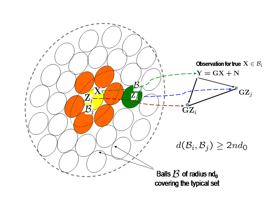
Figure 2: Figure showing the rate distortion cover by balls ${\cal B}$ of radius $\sqrt{nd_{0}}$. The ML decoding over the set of rate distortion quantization points (identified as centers of the distortion balls) consists of mapping $\mathbf{Y}$ to the correct distortion ball for $\mathbf{X}$ using a minimum distance decoder. Shown in the figure is a pair-wise error event for mapping $\mathbf{X}\in{\cal B}_{i}$ to quantization point $\mathbf{Z}_{j}\in{\cal B}_{j}$ that is at a set distance of $2nd_{0}$ from ${\cal B}_{i}$ to which $\mathbf{X}$ belongs.

For the case of squared distortion and covering via spheres of average radius $d_{0}$, it turns out that the worst case $\mathbf{X}$ is given by $\mathbf{X}=\frac{3\mathbf{Z}_{i}+\mathbf{Z}_{j}}{4}$ and $\|\mathbf{Z}_{i}-\mathbf{Z}_{j}\|=4\sqrt{nd_{0}}$. Plugging this value in the expression we have for the worst case pairwise probability of error that

$$\mathbb{P}_{e}(i,j)\leq\mathbb{P}\left\{N\geq\frac{\sqrt{\textit{SNR}}\|\mathbf{G}(\mathbf{Z}_{i}-\mathbf{Z}_{j})\|}{4}\right\}\leq\exp\left\{-\frac{\textit{SNR}\|\mathbf{G}(\mathbf{Z}_{i}-\mathbf{Z}_{j})\|^{2}}{32}\right\}$$

where the second inequality follows by the standard upper bound to the error function. Now we apply the union bound over the set of rate distortion quantization points $\mathbf{Z}_{j}$ minus the set of points that are the neighbors of $\mathbf{Z}_{i}$ (see figure 2). The maximum number of such points is given by $N_{\epsilon}(n,d_{0})=2^{n(R_{X}(d_{0})+\epsilon)}$, where $R_{X}(d_{0})$ is the scalar rate distortion function, [18]. Hence we have,

$$\mathbb{P}(\|\hat{\mathbf{X}}-\mathbf{X}\|^{2}\geq 2nd_{0}\mid\mathbf{X}\in\bigcup_{i}{\cal B}_{i})\leq\exp\left\{-\frac{\textit{SNR}\|\mathbf{G}(\mathbf{Z}_{i}-\mathbf{Z}_{j})\|^{2}}{32}\right\}2^{n(R_{X}(d_{0})+\epsilon)}$$

with $\|\mathbf{Z}_{i}-\mathbf{Z}_{j}\|=4\sqrt{nd_{0}}$. To finish the proof we note that with probability $(1-\epsilon)$, the signal $\mathbf{X}$ belongs to one of the balls ${\cal B}_{j}$. Thus taking expectations with respect to $\mathbf{X}$ the result follows. ∎

5 Approximate Recovery: Bayesian Bounds

In this paper we will consider the following mixture model for explicit evaluation of the bounds.

$$\mathbf{X}_{i}\stackrel{{\scriptstyle d}}{{\sim}}P_{X}=\alpha{\cal N}(\mu_{1},\sigma_{1}^{2})+(1-\alpha){\cal N}(\mu_{0},\sigma_{0}^{2})$$ (33)

i.e., each component $X_{i}$ of $\mathbf{X}$ is IID $P_{X}$ defined above. It is easy to see that for $\mu_{1}=1$, $\mu_{0}=0$ for $\sigma_{0}=0$ this mixture model for large enough $n$ results in an approximately $k=\alpha n$ sparse sequence. We use $\sigma_{1}=0$ to model a binary discrete case and $\sigma_{1}=1$ to model a continuous valued case. It is worth pointing out that this model has been used previously in several papers, e.g. see [22, 14] to probabilistically model sparse signals.

5.1 Discrete $\mathbf{X}$: Support recovery

It is easy to see that using a binary signal model for $\mathbf{X}$ one can address the support recovery problem in the Bayesian setting. Under this case $\mathbf{X}$ is drawn IID according to,

$$P_{X}=\alpha\delta(X-\beta)+(1-\alpha)\delta(X)\,,:\,\,\alpha\leq 0.5$$ (34)

where, $\delta(\cdot)$ is the usual singular measure. Note that it follows from Asymptotic Equipartition Property (AEP), see [18], that asymptotically the $n$-dimensional probability distribution uniformly concentrates on the set of exactly $k$-sparse sequences $\Xi_{\{0,\beta\}}^{\alpha n}$, i.e. given $\epsilon>0,\exists n$ such that $P_{X^{n}}\left(\Xi_{\{0,\beta\}}^{\alpha n}\right)\geq 1-\epsilon$. Thus these bounds can be compared to the worst-case setup of Section 3 when $\mathbf{X}\in\Xi_{\{0,\beta\}}^{k}\,,k=\alpha n$. For this discrete case we have the following main results stated in terms of the scalar rate distortion function $R_{X}(d_{0})$ with Hamming distance as the distortion measure. Note that for this case $R_{X}(d_{0})=H_{2}(\alpha)-H_{2}(d_{0}):\,d_{0}\leq\alpha$.

Theorem 5.1.

Consider the input noise model of Equation (2) and the binary model for $\mathbf{X}$ as described above. Then,

• Necessity: Asymptotically as $n\rightarrow\infty$ if $m\leq\dfrac{nR_{X}(d_{0})}{0.5\log(1+\alpha\beta^{2}\textit{SNR})}$ there does not exist any algorithm that recovers the signal to within an average Hamming distortion of $d_{0}$.

• Sufficiency: Asymptotically as $n\rightarrow\infty$, it is sufficient that $m\geq\dfrac{nR_{X}(d_{0}/2)}{0.5\log(1+\frac{d_{0}\beta^{2}\textit{SNR}}{2})}$ for the constructive ML estimator of section 4.2 to reliably recover the signal to within Hamming distortion of $d_{0}$.

Proof.

To prove part (a) note that from Lemma 4.2 for the probability of error to approach zero implies that the numerator in the lower bound approach zero. This implies that we need,

$$\frac{n}{m}\leq\dfrac{\frac{1}{m}\mathbb{I}(\mathbf{X};\mathbf{Y}|\mathbf{G})}{R_{X}(d_{0})-\frac{1}{n}-\frac{\log nd_{0}}{n}}$$ (35)

To this end recall that $\mathbf{Y}=\mathbf{G}(\mathbf{X}+\frac{1}{\sqrt{\textit{SNR}}}\mathbf{N})$. Consider the SVD of $\mathbf{G}=\mathbf{U}\mathbf{S}\mathbf{V}^{*}$, where $\mathbf{U},\,\mathbf{V}$ are orthonormal matrices and $\mathbf{S}=[\mathbf{D}\,\,\,\mathbf{0}]$, with $\mathbf{D}$ a positive diagonal matrix. From [20] it follows that $\mathbf{U},\,\mathbf{S},\,\mathbf{V}$ are independent random matrices. Furthermore $\mathbf{U}$ and $\mathbf{V}$ are isotropically random. By linearly transforming $\mathbf{Y}$ by pre-multiplying by $\mathbf{D}^{-1}\mathbf{U}^{*}$ we get an equivalent system of equations with

$$\tilde{\mathbf{Y}}=\mathbf{V}_{1}^{*}\mathbf{X}+\frac{1}{\sqrt{\textit{SNR}}}\mathbf{V}_{1}^{*}\mathbf{N}$$ (36)

where $\mathbf{V}_{1}^{*}$ is the matrix formed from the first $m$ rows of $\mathbf{V}^{*}$. Now note that since the rows of $\mathbf{V}_{1}^{*}$ are orthogonal and normalized $\tilde{\mathbf{N}}=\frac{1}{\sqrt{\textit{SNR}}}\mathbf{V}_{1}^{*}\mathbf{N}$ is IID Gaussian with each component having zero mean and variance $1/SNR$. This transformation implies that $\mathbb{I}(\mathbf{X};\mathbf{Y}|\mathbf{G})=\mathbb{I}(\tilde{\mathbf{Y}};\tilde{\mathbf{X}}|\mathbf{V}_{1})$ since $\mathbf{V}$ is independent of $\mathbf{U}$ and $\mathbf{S}$. Now by direct computation it follows that,

$$\mathbf{E}_{\mathbf{V}}\mathbb{I}(\tilde{\mathbf{Y}};\tilde{\mathbf{X}}\mid\mathbf{V}_{1})\leq h(\tilde{\mathbf{Y}}\mid\mathbf{V}_{1})-h(\tilde{\mathbf{Y}}\mid\mathbf{V},\tilde{\mathbf{X}})\leq\frac{m}{2}\log(1+\textit{SNR}\alpha\beta^{2})$$

where to get the last inequality we have used the fact that $h(\tilde{\mathbf{Y}}\mid\mathbf{V},\tilde{\mathbf{X}})$ is the entropy of noise $\tilde{\mathbf{N}}$ and for the first term, $h(\tilde{\mathbf{Y}}\mid\mathbf{V}_{1})$, we have used the fact that a Gaussian distribution maximizes the entropy over all other random variables with zero mean and identical variance [18]. Finally, for sufficiently large $n$ the term $\frac{1}{n}+\frac{\log nd_{0}}{n}$ can be made arbitrarily small and the result follows.

We will now prove part (b). In order to simplify the derivation we again focus on Equation (36). Following the proof of Lemma 4.3 the pairwise error can now be computed as follows

$$\mathbb{P}_{e}(i,j) \leq\mathbb{P}\left\{N\geq\frac{\sqrt{\textit{SNR}}\|\mathbf{V}_{1}^{*}(\mathbf{Z}_{i}-\mathbf{Z}_{j})\|}{4}\left|\right.\mathbf{V}_{1}\right\}\leq\exp\left\{-\frac{\textit{SNR}\|\mathbf{V}_{1}^{*}(\mathbf{Z}_{i}-\mathbf{Z}_{j})\|^{2}}{32}\right\}$$ (37)

To compute the error probability we will need to take the expectation over $\mathbf{V}_{1}$ and apply the union bound to bound the error probability over all error patterns. To simplify the expectation over $\mathbf{V}_{1}$ we let,

$$\phi(\mathbf{D},\mathbf{V}_{1})=\exp\left\{-\frac{\textit{SNR}\|\mathbf{D}\mathbf{V}_{1}^{*}(\mathbf{Z}_{i}-\mathbf{Z}_{j})\|^{2}}{32}\right\}$$ (38)

where, $\mathbf{D}$ is a positive diagonal random matrix independent of $\mathbf{V}_{1}^{*}$. Note that our problem reduces to bounding expectation of $\phi(I_{m},\mathbf{V}_{1})$ over $\mathbf{V}_{1}$. Note that when $\sigma_{\max}(\mathbf{D})\leq 1$ we have $\phi(I_{m},\mathbf{V}_{1})\leq\phi(\mathbf{D},\mathbf{V}_{1})$. Next, note that trivially we have,

$$\phi(I_{m},\mathbf{V}_{1}))I_{\{\sigma_{\max}(\mathbf{D})\leq 1\}}\leq\phi(\mathbf{D},\mathbf{V}_{1})I_{\{\sigma_{\max}(\mathbf{D})\leq 1\}}+\phi(\mathbf{D},\mathbf{V}_{1})I_{\{\sigma_{\max}(\mathbf{D})\geq 1\}}$$ (39)

where $I_{\{\cdot\}}$ denotes the indicator function. Consequently, we can take expectations over the two independent matrices $\mathbf{D}$ and $\mathbf{V}_{1}$ to obtain,

$$E_{\mathbf{V}_{1}}(\phi(I_{m},\mathbf{V}_{1})))Prob(\sigma_{\max}(\mathbf{D})\leq 1)\leq E_{\mathbf{D},\mathbf{V}_{1}}\exp\left\{-\frac{\textit{SNR}\|\mathbf{D}\mathbf{V}_{1}^{*}(\mathbf{Z}_{i}-\mathbf{Z}_{j})\|^{2}}{32}\right\}$$ (40)

Note that we can introduce a isotropically random unitary matrix $\mathbf{U}$, namely, $\exp\left\{-\frac{\textit{SNR}}{32}\|\mathbf{D}\mathbf{V}_{1}^{*}(\mathbf{Z}_{i}-\mathbf{Z}_{j})\|^{2}\right\}=\exp\left\{-\frac{\textit{SNR}}{32}\|\mathbf{U}\mathbf{D}\mathbf{V}_{1}^{*}(\mathbf{Z}_{i}-\mathbf{Z}_{j})\|^{2}\right\}$ without modifying the result. Now the matrix $\mathbf{H}=\mathbf{U}\mathbf{D}\mathbf{V}_{1}^{*}$ can be identified by a suitable IID Gaussian matrix when $\mathbf{U},\,\mathbf{D},\,\mathbf{V}$ are chosen independently and $\mathbf{U}$ and $\mathbf{V}$ are chosen uniformly from set of all unitary matrices; the positive diagonal matrix $\mathbf{D}$ is distributed according to the distribution of singular values of a Gaussian matrix. To ensure a tight approximation we need to choose a Gaussian matrix such that $\mathbb{P}(\sigma_{\max}(\mathbf{D})\leq 1)$ approaches one. This can be accomplished by choosing $\mathbf{H}$ as an IID Gaussian ensemble with each component $h_{ij}\stackrel{{\scriptstyle d}}{{\sim}}{\cal N}(0,{1\over(1+\sqrt{m/n})n})$. Then following similar steps as in the proof of Lemma 4.3 we arrive at a similar upper bound,

$$\mathbb{P}(\|\hat{\mathbf{X}}-\mathbf{X}\|^{2}\geq 2nd_{0})\leq(1-\epsilon)\exp\left\{-\frac{\textit{SNR}\|\mathbf{H}(\mathbf{Z}_{i}-\mathbf{Z}_{j})\|^{2}}{32}\right\}2^{n(R_{X}(d_{0})+\epsilon)}+\epsilon$$

where, $\|\mathbf{Z}_{i}-\mathbf{Z}_{j}\|=4\sqrt{nd_{0}}$. Since $\epsilon$ is arbitrary, the result then follows by taking expectation with respect to $\mathbf{H}$ and using the moment generating function of the $\chi^{2}$ random variable, [23]. ∎

Theorem 5.2.

Consider the output noise model of Equation (1) and the binary model for $\mathbf{X}$ as described above. Then,

• Necessity: Asymptotically as $n\rightarrow\infty$ if $m\leq\dfrac{nR_{X}(d_{0})}{0.5\log(1+\frac{n}{m}\alpha\beta^{2}\textit{SNR})}$ there does not exist any algorithm that recovers the signal to within an average Hamming distortion of $d_{0}$.

• Sufficiency: Asymptotically as $n\rightarrow\infty$ it is sufficient that $m\geq\dfrac{nR_{X}(d_{0}/2)}{0.5\log(1+\frac{n}{m}\frac{d_{0}\beta^{2}\textit{SNR}}{2})}$ for the constructive ML estimator of section 4.2 to reliably recover the signal to within Hamming distortion of $d_{0}$.

Proof.

The proof of part (a) follows along the same lines as that of 5.1 with the following modification to the upper bound of the mutual information expression,

$$\mathbf{E}_{\mathbf{G}}\mathbb{I}(\mathbf{X};\mathbf{Y}|\mathbf{G})\leq\frac{m}{2}\log(1+\frac{n\alpha\beta^{2}\textit{SNR}}{m})$$ (41)

The proof of part (b) follows from the upper bound to the probability of error in Lemma 4.3 by taking expectation with respect to $\mathbf{G}$ and using the moment generating function of the $\chi^{2}$ random variable, see [23]. ∎

We will now reduce the implicit expression in the above Lemma to derive some explicit conditions on the number of measurements $m$. To this end we have the following corollary.

Corollary 5.1.

Consider the output noise model of Equation (1) and the binary model for $\mathbf{X}$ as described above. Then, (a) Asymptotically as $n\rightarrow\infty$ if $\textit{SNR}\leq\frac{2R_{X}(d_{0})}{\alpha\beta^{2}}$ and $m\leq 2nR_{X}(d_{0})$ there exists no algorithm that can recover $\mathbf{X}$ to within an average Hamming distortion of $d_{0}$; (b) On the other hand asymptotically as $n\rightarrow\infty$ it is sufficient that $\textit{SNR}\geq\frac{200R_{X}(d_{0}/2)}{d_{0}\beta^{2}}$ with $m\geq 2.08nR_{X}(d_{0}/2)$ for the constructive ML estimator of section 4.2 to recover $\mathbf{X}$ to within an average Hamming distortion of $d_{0}$.

Proof.

To begin with we will focus on the sufficient conditions. Denote by $c=\frac{nR_{X}(d_{0}/2)}{m}$. Also let $\eta=\frac{d_{0}\beta^{2}\textit{SNR}}{2R_{X}(d_{0}/2)}$. Then from part (b) of Theorem 5.2 we have as a sufficient condition that,

$$f(c)=0.5\log(1+c\eta)-c\geq 0$$ (42)

In particular we want to find $\max\{c|f(c)\geq 0\}$. To this end note that $f(c)=0$ at $c=0$. Also for there to exist any positive $c$ such that $f(c)>0$ it is required that $\eta\geq 2$. In particular $\eta\geq 2$ is the condition for a positive derivative near zero. This implies that $\frac{d_{0}\beta^{2}\textit{SNR}}{2R_{X}(d_{0}/2)}\geq 2$ or $\textit{SNR}\geq\frac{4R_{X}(d_{0}/2)}{d_{0}\beta^{2}}$. Given that this condition is satisfied, $c=\frac{1-2/\eta}{2}$ lies in the feasible region. Therefore $m=\frac{2}{1-2/\eta}nR_{x}(d_{0}/2)\approx 2nR_{X}(d_{0}/2)$ is a sufficient condition for reliable recovery for some sufficiently large $\eta>2$, i.e. for $\textit{SNR}\geq\frac{4R_{X}(d_{0}/2)}{d_{0}\beta^{2}}$ . In particular if we choose $\eta=100$ then $\textit{SNR}\geq\frac{200R_{X}(d_{0}/2)}{d_{0}\beta^{2}}$ and $m\geq 2.08nR_{X}(d_{0}/2)$ is sufficient for reliable recovery.

Analyzing part (a) of the Theorem 5.2 in a similar manner, one can show that if $\textit{SNR}\leq\frac{2R_{X}(d_{0})}{\alpha\beta^{2}}$ and $m\leq 2nR_{X}(d_{0})$ there exits no algorithm that can reliably recover $\mathbf{X}$ to within the desired distortion level. ∎

Remark 5.1.

One immediate observation from the above analysis is that unlike the worst case set-up one can indeed tradeoff the number of measurements with distortion in the Bayesian set-up.

5.2 Continuous $\mathbf{X}$: $\ell_{2}$ recovery

Under this case $\mathbf{X}$ is drawn IID according to,

$$P_{X}=\alpha{\cal N}(0,\beta^{2})+(1-\alpha)\delta(X)$$ (43)

For this case we have the following main results. The results are stated in terms of the scalar rate distortion function $R_{X}(d_{0})$ given by $R_{X}(d_{0})=H_{2}(\alpha)+\frac{\alpha}{2}\log\frac{\alpha}{d_{0}}:\,d_{0}<\alpha$, (see section 8.4 for the derivation of this result). Notice in the following that in contrast to the discrete case where $d_{0}\leq\alpha$ here we impose $d_{0}\leq\alpha/2$ and for reasonable reconstruction one typically desires $d_{0}=\epsilon\alpha$ for some small $\epsilon>0$. The reason that we require $d_{0}\leq\frac{\alpha}{2}$ is due to the additional term of $K(n,d_{0})$ in the modified Fano’s inequality 4.1 which appears in the continuous setting.

Theorem 5.3.

Consider the input noise model of Equation (2) and the mixture model for $\mathbf{X}$ as described above. Then,

• Necessity: Asymptotically as $n\rightarrow\infty$ if $m\leq\dfrac{n(R_{X}(d_{0})-\frac{\alpha}{2}\log 2)}{0.5\log(1+\alpha\beta^{2}\textit{SNR})}$ there does not exist any algorithm that recovers the signal to within an average $\ell_{2}$ distortion of $d_{0}$.

• Sufficiency: Asymptotically as $n\rightarrow\infty$ it is sufficient that $m\geq\dfrac{nR_{X}(d_{0}/2)}{0.5\log(1+\frac{d_{0}\beta^{2}\textit{SNR}}{2})}$ for the constructive ML estimator of section 4.2 to reliably recover the signal to within an average $\ell_{2}$ distortion of $d_{0}$.

Proof.

For part (a) first note that from Theorem 5.1 we have $\mathbf{E}_{\mathbf{G}}\mathbb{I}(\mathbf{X};\mathbf{Y}|\mathbf{G})\leq\frac{m}{2}\log(1+\beta^{2}\alpha\textit{SNR})$. From Lemma 4.1 it follows that for feasibility of recovery to with distortion $d_{0}$ (asymptotically) it is required that,

$$\frac{n}{m}\leq\frac{\frac{1}{m}\mathbf{E}_{\mathbf{G}}\mathbb{I}(\mathbf{X};\mathbf{Y}|\mathbf{G})}{R_{X}(d_{0})-K(d_{0},n)}$$ (44)

The result then follows by noting that $|K(d_{0},n)-0.5\alpha\log 2|<\epsilon$ with $\epsilon$ arbitrarily small for large enough $n$, see e.g. [24]. Note that for the case at hand in order for the expression $R_{X}(d_{0})-K(d_{0},n)$ to remain positive and hence meaningful, $d_{0}\leq\alpha/2$. The proof of part (b) follows exactly along the same lines as the proof of part (b) in Theorem 5.1. ∎

Note that unlike the case of support recovery where the number of measurements had to grow with signal dimension even with SNR of $\log(n)$ here we see that the number of measurements does scale with the distortion for moderate signal to noise ratios. This maybe acceptable in cases where either a probability model for the signal set is available.

Theorem 5.4.

Consider the output noise model of Equation (1) and the mixture model for $\mathbf{X}$ as described above. Then,

• Necessity: Asymptotically as $n\rightarrow\infty$ if $m\leq\dfrac{n(R_{X}(d_{0})-\frac{\alpha}{2}\log 2)}{0.5\log(1+\frac{n}{m}\alpha\beta^{2}\textit{SNR})}$ there does not exist any algorithm that recovers the signal to within an average $\ell_{2}$ distortion of $d_{0}$.

• Sufficiency: Asymptotically as $n\rightarrow\infty$ it is sufficient that $m\geq\dfrac{nR_{X}(d_{0}/2)}{0.5\log(1+\frac{n}{m}\frac{d_{0}\beta^{2}\textit{SNR}}{2})}$ for the constructive ML estimator of section 4.2 to reliably recover the signal to within an average $\ell_{2}$ distortion of $d_{0}$.

Proof.

The proof is similar to the proof of Theorem 5.3. ∎

It is easy to see that Corollary 5.1 holds true for this case too with appropriate modifications to the necessary conditions in terms of $R_{X}(d_{0})-\frac{\alpha}{2}\log 2$ instead of $R_{X}(d_{0})$.

5.3 Comparison between Worst-Case and Bayesian Setups

Based on the worst-Case and Bayesian results we can comment on the main differences. The situation is slightly complicated since we considered two different types of distortions in these cases. We recall the items (A)—(D) listed in the beginning of Section 4 as a means for comparison. Note that by adopting a Bayesian setup we no longer need that the minimum singular value of sub-matrices of $\mathbf{G}$ be uniformly bounded away from zero. This can be attributed to the fact that we are taking expectation with respect to $\mathbf{G}$ in Equation (29). However, note that the number of quantization points $N_{\epsilon}(n,d_{0})$ in Theorem 8.1 will go to infinity if we insist on nearly exact support recovery. Second, note that the measurements do scale with the distortion-level, larger the admissible distortion, smaller the number of measurements. This is even more surprising for input noise models since in the worst-case setup we required the number of measurements to scale with signal dimension. Finally, for signal reconstruction to within a distortion level $d_{0}$ we only need a constant SNR in contrast to the worst-case setup. However, this issue can be attributed to the fact that our mean-squared distortion metric is less stringent in comparison to support errors.

6 Appendix

6.1 Proof of Lemma 3.3

Consider any arbitrary $\mathbf{G}$ and $\mathbf{N}$. Let for each $\mathbf{X}\in\Xi_{\beta}^{\{k\}}$ denote by $\mathbb{P}_{\mathbf{X}}$ the observed distribution of $\mathbf{Y}$ given $\mathbf{X}$ as induced by the relation $\mathbf{Y}=\mathbf{G}\mathbf{X}+\mathbf{N}$. We next consider the equivalence class of all sequences with the same support and lump the corresponding class of observation probabilities into a single composite hypothesis, i.e.,

$$[\mathbf{X}]=\{\mathbf{X}^{\prime}\in\Xi_{\beta}^{\{k\}}\mid\mbox{Supp}(\mathbf{X}^{\prime})=\mbox{Supp}(\mathbf{X})\}$$ (45)

Each equivalence class bears a one-to-one correspondence with binary valued k-sparse sequences,

$$\Xi_{\{0,\beta\}}^{\{k\}}=\{\mathbf{X}\in\Xi_{\beta}^{\{k\}}\mid X_{i}=\beta,\,\,i\in\mbox{Supp}(\mathbf{X})\}$$ (46)

Our task is to lower bound the worst-case error probability

$$\mathbb{P}_{e|\mathbf{G}}=\min_{\hat{\mathbf{X}}}\max_{\mathbf{X}\in\Xi_{\beta}^{\{k\}}}\mathbb{P}_{\mathbf{X}}([\hat{\mathbf{X}}]\neq[\mathbf{X}]|\mathbf{G})$$ (47)

Now note that,

$$\max_{\mathbf{X}\in\Xi_{\beta}^{\{k\}}}\mathbb{P}_{\mathbf{X}}([\hat{\mathbf{X}}]\neq[\mathbf{X}]|\mathbf{G})\geq\max_{\mathbf{X}\in\Xi_{\{0,\beta\}}^{\{k\}}}\mathbb{P}_{\mathbf{X}}([\hat{\mathbf{X}}]\neq[\mathbf{X}]|\mathbf{G})=\max_{\mathbf{X}\in\Xi_{0,\beta}^{\{k\}}}\mathbb{P}_{\mathbf{X}}(\hat{\mathbf{X}}\neq\mathbf{X},\,\,\hat{\mathbf{X}}\in\Xi_{\{0,\beta\}}|\mathbf{G})$$ (48)

This implies that

$$\mathbb{P}_{e|\mathbf{G}} =\min_{\hat{\mathbf{X}}\in\Xi_{\beta}^{\{k\}}}\max_{\mathbf{X}\in\Xi_{\beta}^{\{k\}}}\mathbb{P}_{\mathbf{X}}\{\mbox{Supp}(\hat{\mathbf{X}})\neq\mbox{Supp}(\mathbf{X})|\mathbf{G}\}$$ (49)

$$\geq\min_{\hat{\mathbf{X}}\in\Xi_{\beta}^{\{k\}}}\max_{\mathbf{X}\in\Xi_{\{0,\beta\}}^{\{k\}}}\mathbb{P}_{\mathbf{X}}(\hat{\mathbf{X}}\neq\mathbf{X},\,\,\hat{\mathbf{X}}\in\Xi_{\{0,\beta\}}^{\{k\}}|\mathbf{G})$$ (50)

$$=\min_{\hat{\mathbf{X}}\in\Xi_{\{0,\beta\}}^{\{k\}}}\max_{\mathbf{X}\in\Xi_{\{0,\beta\}}^{\{k\}}}\mathbb{P}_{\mathbf{X}}(\hat{\mathbf{X}}\neq\mathbf{X},\,\,\hat{\mathbf{X}}\in\Xi_{\{0,\beta\}}^{\{k\}}|\mathbf{G})$$ (51)

$$\geq\min_{\hat{\mathbf{X}}\in\Xi_{\{0,\beta\}}^{\{k\}}}\max_{\mathbf{X}\in\Xi_{\{0,\beta\}}^{{}^{\prime}}}\mathbb{P}_{\mathbf{X}}(\hat{\mathbf{X}}\neq\mathbf{X},\,\,\hat{\mathbf{X}}\in\Xi_{\{0,\beta\}}^{\{k\}}|\mathbf{G})$$ (52)

6.2 Proof of Lemma 3.5

Denote by ${\cal E}_{1\omega}$ the error event when a signal from the $\omega$th support set is more likely, i.e.,

$${\cal E}_{1\omega}=\left\{\mathbf{N}:\min_{\omega\in{\cal I}\mathbf{X}_{S_{\omega}}^{\min}\geq\beta/2}\|\mathbf{Y}-\mathbf{G}_{S_{\omega}}\mathbf{X}_{S_{\omega}}\|^{2}\leq\min_{\tilde{\mathbf{X}}}\|\mathbf{Y}-\mathbf{G}_{S_{0}}\tilde{\mathbf{X}}\|^{2},\,\,\omega\not=0,\,\,\right\}$$ (53)

In the following we will drop stating the obvious fact that $\omega\in{\cal I}$. Now note that,

$${\cal E}_{1}=\bigcup_{\omega\not=0}{\cal E}_{1\omega}$$ (54)

We first upperbound ${\cal E}_{1\omega}$ by a more manageable event, namely,

$${\cal F}_{\omega}=\left\{\mathbf{N}:\min_{\mathbf{X}_{S_{0^{c},\omega}}^{\min}\geq\beta/2}\min_{\mathbf{X}_{S_{0,\omega}}}\|\mathbf{Y}-\mathbf{G}_{S_{0,\omega}}\mathbf{X}_{S_{0,\omega}}-\mathbf{G}_{S_{0^{c},\omega}}\mathbf{X}_{S_{0^{c},\omega}}\|^{2}\leq\min_{\tilde{\mathbf{X}}}\|\mathbf{Y}-\mathbf{G}_{S_{0}}\tilde{\mathbf{X}}\|^{2},\,\,\omega\not=0\right\}$$ (55)

It is clear that,

$${\cal E}_{1\omega}\subset{\cal F}_{\omega}$$ (56)

This is because the signal on the common support $S_{0,\omega}$ is relaxed to take on any value and not necessarily those that are bounded away from zero by $\beta/2$. We will now simplify the events in ${\cal F}_{\omega}$ by analytically carrying out the unconstrained minimizations. Recall that $\mathbf{Y}=\mathbf{G}\mathbf{X}_{0}+\mathbf{N}$. Let $\mathbf{X}_{S_{0}}^{0}$ denote the true signal $\mathbf{X}_{0}$ restricted to its support. Then $\mathbf{Y}=\mathbf{G}_{S_{0}}\mathbf{X}_{S_{0}}^{0}$. Note that $\mathbf{X}_{S_{0}}^{0}$ is composed of $\mathbf{X}_{S_{0,\omega}}^{0}$ corresponding to the overlap and $\mathbf{X}_{0,\omega^{c}}^{0}$ corresponding to the misses. We have the following Lemma.

Lemma 6.1.

For $m\geq 2k+1$

$${\cal F}_{\omega}\subset\tilde{\cal F}_{\omega}=\bigcup_{\mathbf{X}_{S_{0^{c},\omega}}^{\min}\geq\beta/2,\mathbf{X}_{S_{0,\omega^{c}}}^{0,\min}\geq\beta}\left\{\mathbf{N}:2\mathbf{N}^{T}\mathbf{\Pi}_{1}\mathbf{G}^{\prime}\mathbf{X}^{\prime}\geq\|\mathbf{\Pi}_{1}\mathbf{G}^{\prime}\mathbf{X}^{\prime}\|^{2},\,\,\right\}$$ (57)

where

$$\mathbf{\Pi}_{1}=(\mathbf{I}-\mathbf{G}_{S_{0,\omega}}(\mathbf{G}_{S_{0,\omega}}^{T}\mathbf{G}_{S_{0,\omega}})^{-1}\mathbf{G}_{S_{0,\omega}}^{T})$$ (58)

is a projection operator and

$$\mathbf{G}^{\prime}=[\mathbf{G}_{S_{0^{c},\omega}}\mathbf{G}_{S_{0,\omega^{c}}}],\mathbf{X}^{\prime}=\begin{bmatrix}-\mathbf{X}_{S_{0^{c},\omega}}\\ \mathbf{X}_{S_{0,\omega^{c}}}^{0}\end{bmatrix},\,\,\mathbf{X}_{S_{0^{c},\omega}}^{\min}\geq\beta/2,\,\,\mathbf{X}_{S_{0,\omega^{c}}}^{0,\min}\geq\beta$$ (59)

Proof.

Consider the error region,

$${\cal F}_{\omega}=\left\{\mathbf{N}:\min_{\mathbf{X}_{S_{0^{c},\omega}}^{\min}\geq\beta/2}\min_{\mathbf{X}_{S_{0,\omega}}}\|\mathbf{Y}-\mathbf{G}_{S_{0,\omega}}\mathbf{X}_{S_{0,\omega}}-\mathbf{G}_{S_{0^{c},\omega}}\mathbf{X}_{S_{0^{c},\omega}}\|^{2}\leq\min_{\tilde{\mathbf{X}}}\|\mathbf{Y}-\mathbf{G}_{S_{0}}\tilde{\mathbf{X}}\|^{2},\,\,\omega\not=0\right\}$$ (60)

Fixing $\mathbf{X}_{S_{0^{c},\omega}}$ we perform the inner minimization first on the L.H.S in the above equation. It can be shown that the inner minimum is achieved at,

$$\mathbf{X}_{S_{0,\omega}}^{0}-\mathbf{X}_{S_{0,\omega}}=-(\mathbf{G}_{S_{0,\omega}}^{T}\mathbf{G}_{S_{0,\omega}})^{-1}\mathbf{G}_{S_{0,\omega}}^{T}(\mathbf{N}+\mathbf{G}_{S_{0,\omega^{c}}}\mathbf{X}_{S_{0,\omega^{c}}}^{0}-\mathbf{G}_{S_{0^{c},\omega}}\mathbf{X}_{S_{0^{c},\omega}})$$ (61)

Also the unconstrained minimum on the R.H.S. is given by,

$$\min_{\tilde{\mathbf{X}}}||(\mathbf{Y}-\mathbf{G}_{S_{0}}\tilde{\mathbf{X}})||^{2}=\mathbf{N}^{T}\mathbf{\Pi}_{0}\mathbf{N}$$ (62)

where

$$\mathbf{\Pi}_{0}=(\mathbf{I}-\mathbf{G}_{S_{0}}(\mathbf{G}_{S_{0}}^{T}\mathbf{G}_{S_{0}})^{-1}\mathbf{G}_{S_{0}}^{T})$$ (63)

is a projection operator. Substituting these results in the expression for ${\cal F}_{\omega}$ we obtain,

$${\cal F}_{\omega}= \left\{\mathbf{N}:\min_{\mathbf{X}_{S_{0^{c},\omega}}^{\min}\geq\beta/2}(\mathbf{G}^{\prime}\mathbf{X}^{\prime})^{T}\mathbf{\Pi}_{1}\mathbf{G}^{\prime}\mathbf{X}^{\prime}-2\mathbf{N}^{T}\mathbf{\Pi}_{1}\mathbf{G}^{\prime}\mathbf{X}^{\prime}+\mathbf{N}^{T}(\mathbf{\Pi}_{0}-\mathbf{\Pi}_{1})\mathbf{N}\leq 0\right\}$$ (64)

A simple application of the matrix lemma shows that $(\mathbf{\Pi}_{0}-\mathbf{\Pi}_{1})$ is a positive semi-definite matrix. This implies $\mathbf{N}^{T}(\mathbf{\Pi}_{0}-\mathbf{\Pi}_{1})\mathbf{N}\geq 0$, $\forall\mathbf{N}$. Ignoring this non-negative term can only increase the probability of error. Therefore ignoring this term we obtain,

$${\cal F}_{\omega}= \left\{\mathbf{N}:\min_{\mathbf{X}_{S_{0,\omega^{c}}}^{\min}\geq\beta/2}(\mathbf{G}^{\prime}\mathbf{X}^{\prime})^{T}\mathbf{\Pi}_{1}\mathbf{G}^{\prime}\mathbf{X}^{\prime}-2\mathbf{N}^{T}\mathbf{\Pi}_{1}\mathbf{G}^{\prime}\mathbf{X}^{\prime}\leq 0\right\}$$ (65)

$$\subseteq\bigcup_{\mathbf{X}_{S_{0^{c},\omega}}^{\min}\geq\beta/2,\mathbf{X}_{S_{0,\omega^{c}}}^{0,\min}\geq\beta}\left\{\mathbf{N}:(\mathbf{G}^{\prime}\mathbf{X}^{\prime})^{T}\mathbf{\Pi}_{1}\mathbf{G}^{\prime}\mathbf{X}^{\prime}-2\mathbf{N}^{T}\mathbf{\Pi}_{1}\mathbf{G}^{\prime}\mathbf{X}^{\prime}\leq 0\right\}$$ (66)

$$=\bigcup_{\mathbf{X}_{S_{0^{c},\omega}}^{\min}\geq\beta/2,\mathbf{X}_{S_{0,\omega^{c}}}^{0,\min}\geq\beta}\left\{\mathbf{N}:2\mathbf{N}^{T}\mathbf{\Pi}_{1}\mathbf{G}^{\prime}\mathbf{X}^{\prime}\geq\|\mathbf{\Pi}_{1}\mathbf{G}^{\prime}\mathbf{X}^{\prime}\|^{2}\right\}={\tilde{\cal F}}_{\omega}$$ (67)

where the last equality follows from the fact that $\mathbf{\Pi}_{1}$ is a projection. Now note that if any column of $\mathbf{G}^{\prime}$ falls into the null space of $\mathbf{G}_{S_{0,\omega}}$ then probability of the event ${\cal F}_{\omega}$ is $1$ and therefore the probability of error is $1$ in the worst case. This will not happen as long as $\mathbf{G}$ is full rank and $m\geq 2k+1$. ∎

We now have the following Lemma.

Lemma 6.2.

$$\tilde{\cal F}_{\omega}\subseteq{\cal L}_{\omega}=\bigcup_{j=1}^{L}\left\{\mathbf{N}:2\mathbf{N}^{T}\mathbf{g}_{j}^{{}^{\prime}}X^{\prime}\geq\sigma_{\min}((\mathbf{G}^{\prime})^{T}\mathbf{G}^{\prime})X^{\prime 2},|X^{\prime}|=\beta/2\right\}$$ (68)

where $L=|S_{0^{c},\omega}\cup S_{0,\omega^{c}}|$ is the total number of location errors and, $\sigma_{\min}((\mathbf{G}^{\prime})^{T}\mathbf{G}^{\prime})$ is the minimum singular value of the matrix $(\mathbf{G}^{\prime})^{T}\mathbf{G}^{\prime}$.

Proof.

Let $\tilde{\mathbf{G}}=\mathbf{\Pi}_{1}\mathbf{G}^{\prime}$. Then note that for any $\mathbf{X}^{\prime}$,

$$\left\{\tilde{\mathbf{N}}:2\mathbf{N}^{T}\tilde{\mathbf{G}}\mathbf{X}^{\prime}\geq\|\tilde{\mathbf{G}}\ \mathbf{X}^{\prime}\|^{2}\right\}\subseteq\left\{\mathbf{N}:2\mathbf{N}^{T}\tilde{\mathbf{G}}\mathbf{X}^{\prime}\geq\sigma_{\min}(\tilde{\mathbf{G}}^{T}\tilde{\mathbf{G}})\|\mathbf{X}^{\prime}\|^{2}\right\}$$ (69)

Now note that

$$\tilde{\mathbf{G}}\mathbf{X}^{\prime}=\sum_{j=1}^{L}\tilde{\mathbf{g}}_{j}X^{\prime}_{j}$$

where $\tilde{\mathbf{g}}_{j}$ is the $j$-th column of the matrix $\tilde{\mathbf{G}}$ and $\mathbf{X}^{\prime}=[X^{\prime}_{1},\ldots,X^{\prime}_{j},\ldots,X^{\prime}_{L}]^{T}$. Note also that

$$\|\mathbf{X}^{\prime}\|^{2}=\sum_{j}|X^{\prime}_{j}|^{2}$$

By a simple superposition of events this implies that

$$\tilde{\cal F}_{\omega} \subseteq\bigcup_{\mathbf{X}_{S_{0^{c},\omega}}^{\min}\geq\beta/2,\mathbf{X}_{S_{0,\omega^{c}}}^{0,\min}\geq\beta}\bigcup_{j=1}^{L}\left\{{\mathbf{N}}:2\mathbf{N}^{T}\tilde{\mathbf{g}}_{j}X^{\prime}_{j}\geq\sigma_{\min}(\tilde{\mathbf{G}}^{T}\tilde{\mathbf{G}})|X^{\prime}_{j}|^{2}\right\}$$

$$\subseteq\bigcup_{\mathbf{X}_{S_{0^{c},\omega}}^{\min}\geq\beta/2,\mathbf{X}_{S_{0,\omega^{c}}}^{0,\min}\geq\beta}\bigcup_{j=1}^{L}\left\{\mathbf{N}:2\mathbf{N}^{T}\tilde{\mathbf{g}}_{j}X^{\prime}_{j}\geq\sigma_{\min}(\tilde{\mathbf{G}}^{T}\tilde{\mathbf{G}})|X^{\prime}_{j}|^{2}\right\}$$ (70)

$$\subseteq\bigcup_{j=1}^{L}\left\{\mathbf{N}:2\mathbf{N}^{T}\tilde{\mathbf{g}}_{j}X^{\prime}\geq\sigma_{\min}(\tilde{\mathbf{G}}^{T}\tilde{\mathbf{G}})|X^{\prime}|^{2}:|X^{\prime}|=\beta/2\right\}$$ (71)

where the last inequality follows from the fact all the events with $X^{\prime}\geq\beta/2$ are contained in the event $X^{\prime}=\beta/2$. Now note that since $\mathbf{\Pi}_{1}$ is a projection and $m\geq 2k+1$ and $L\leq 2k$ it implies $\sigma_{min}(\tilde{\mathbf{G}}^{T}\tilde{\mathbf{G}})=\sigma_{min}((\mathbf{G}^{\prime})^{T}\mathbf{G}^{\prime})$. This implies that,

$$\tilde{\cal F}_{\omega} \subseteq\bigcup_{j=1}^{L}\left\{\mathbf{N}:2\mathbf{N}^{T}\tilde{\mathbf{g}}_{j}X^{\prime}\geq\sigma_{\min}(\tilde{\mathbf{G}}^{T}\tilde{\mathbf{G}})|X^{\prime}|^{2}:|X^{\prime}|=\beta/2\right\}$$ (72)

$$=\bigcup_{X^{\prime}=\pm\beta/2}\bigcup_{j=1}^{L}\left\{\mathbf{N}:2\mathbf{N}^{T}\mathbf{g}^{\prime}_{j}X^{\prime}\geq\sigma_{\mathbf{G},\min}((\mathbf{G}^{\prime})^{T}\mathbf{G}^{\prime})|X^{\prime}|^{2}\right\}$$ (73)

Since $L\leq 2k\leq n$ and $\left\{\mathbf{g}^{\prime}_{1},..,\mathbf{g}^{\prime}_{j},...,\mathbf{g}^{\prime}_{L}\right\}=\left\{\mathbf{g}_{i}:i\in S_{0^{c},\omega}\cup S_{0,\omega^{c}}\right\}\subseteq\left\{\mathbf{g}_{1},...,\mathbf{g}_{n}\right\}$,

$${\cal F}_{\omega} \subseteq\bigcup_{X^{\prime}=\pm\beta/2}\bigcup_{j=1}^{n}\left\{\mathbf{N}:2\mathbf{N}^{T}\mathbf{g}_{j}X^{\prime}\geq\sigma_{\mathbf{G},\min}|X^{\prime}|^{2}\right\}$$ (74)

$$={\cal L}_{\omega}$$ (75)

where $\sigma_{\mathbf{G},\min}=\min_{S:|S|\leq 2k}\sigma_{\min}(\mathbf{G}_{S}^{T}\mathbf{G}_{S})$. ∎

The result then follows by noting that,

$${\cal E}_{1}=\bigcup_{\omega}{\cal E}_{1\omega}\subseteq\bigcup_{\omega}{\cal F}_{\omega}\subseteq\bigcup_{\omega}{\cal L}_{\omega}$$ (76)

and replacing the notation $X^{\prime}$ by $X$.

7 Proof of Lemma 3.6

From Lemma 3.5 we have ,

$$\mathbb{P}({\cal E}_{1}) \leq\bigcup_{X=\pm\beta/2}\bigcup_{j=1}^{n}\left\{\mathbf{N}:2\mathbf{N}^{T}\mathbf{g}_{j}X\geq\sigma_{\mathbf{G},\min}\sqrt{\textit{SNR}}|X|^{2}\right\}=\bigcup_{X=\pm\beta/2}\bigcup_{j=1}^{n}\left\{\mathbf{W}:2\mathbf{W}^{T}\mathbf{\Sigma}^{1/2}\mathbf{g}_{j}X\geq\sigma_{\mathbf{G},\min}\sqrt{\textit{SNR}}|X|^{2}\right\}$$

$$=\bigcup_{X=\pm\beta/2}\bigcup_{j=1}^{n}\left\{w:2wX\geq\sqrt{\textit{SNR}}\sigma_{\mathbf{G},\min}\frac{X^{2}}{\sqrt{\mathbf{g}_{j}^{{}^{\prime}}\mathbf{\Sigma}\mathbf{g}_{j}}}\right\}$$

Note that $\mathbf{W}$ is IID normally distributed Gaussian vector and we let $w=\frac{\mathbf{W}^{T}\mathbf{\Sigma}^{1/2}\mathbf{g}_{j}}{\sqrt{\mathbf{g}_{j}^{T}\mathbf{\Sigma}\mathbf{g}_{j}}}$. Next noting that $\|\mathbf{g}_{j}\|=1$ $\forall j$ we have,

$$\left\{w:2wX\geq\sqrt{\textit{SNR}}\sigma_{\mathbf{G},\min}\frac{X^{2}}{\sqrt{\|\mathbf{g}_{j}^{T}\mathbf{\Sigma}\mathbf{g}_{j}\|}}\right\} \subseteq\left\{w:2wX\geq\sqrt{\textit{SNR}}\sigma_{\mathbf{G},\min}\sqrt{\frac{1}{\lambda_{\max}(\mathbf{\Sigma})}}X^{2}\right\}$$ (77)

$$=\left\{w:2wX\geq\sqrt{\textit{SNR}}\sigma_{\mathbf{G},\min}\sqrt{\lambda_{\min}(\mathbf{\Sigma}^{-1})}X^{2}\right\}$$ (78)

We now apply the union bound over all the possible $2n$ error events corresponding to each $j\in\{1,2,...,n\}$ and $X=\pm\beta/2$ and obtain,

$$\mathbb{P}({\cal E}_{1}) \leq\mathbb{P}\left\{w:w\geq\sqrt{\lambda_{\min}(\mathbf{\Sigma}^{-1})}\sigma_{\mathbf{G},min}\frac{\sqrt{\textit{SNR}}\beta}{4}\right\}\exp(\log 2n)$$ (79)

$$=\frac{1}{\sqrt{2\pi}}\int_{\sqrt{\lambda_{\min}(\mathbf{\Sigma}^{-1})}\sigma_{\mathbf{G},\min}\frac{\sqrt{\textit{SNR}}\beta}{4}}^{\infty}\exp(-y^{2}/2)dy\,\cdot\exp(\log 2n)$$ (80)

$$\leq\exp\left\{-\lambda_{\min}(\mathbf{\Sigma}^{-1})\sigma_{\mathbf{G},\min}^{2}\frac{\beta^{2}\textit{SNR}}{32}\right\}\exp\left\{\log 2n\right\}$$ (81)

Note that the probability is only taken over the noise $\mathbf{W}$ ($\mathbf{N}$) as $\mathbf{G}$ is given and is fixed. Here we have used the approximation ${\cal Q}(x)\leq\exp(-x^{2}/2)$ for the standard error function defined as ${\cal Q}(x)=\frac{1}{\sqrt{2\pi}}\int_{x}^{\infty}\exp(-x^{2}/2)dx$.

8 Proof of Lemma 3.7

For any $\mathbf{X}_{0}$ supported on the submatrix $\mathbf{G}_{S_{0}}$ the probability of the error event ${\cal E}_{2}$ is given by,

$$\mathbb{P}({\cal E}_{2})=\mathbb{P}\left\{\mathbf{N}:\|(\mathbf{G}_{S_{0}}^{T}\mathbf{G}_{S_{0}})^{-1}\mathbf{G}_{S_{0}}^{T}\mathbf{N}\|_{\infty}\geq\sqrt{\textit{SNR}}\beta/2\right\}$$ (82)

To this end let $\mathbf{G}_{S_{0}}=\mathbf{U}\mathbf{\Sigma}_{S_{0}}\mathbf{V}^{*},\mathbf{U}\in\mathbb{C}^{m\times k},\mathbf{V}^{*}\in\mathbb{C}^{k\times m}$. Then $(\mathbf{G}_{S_{0}}^{T}\mathbf{G}_{S_{0}})^{-1}\mathbf{G}_{S_{0}}^{T}=\mathbf{U}\mathbf{\Sigma}_{S_{0}}^{-1}\mathbf{V}^{*}$. Then let $\tilde{\mathbf{N}}=\mathbf{V}^{*}\mathbf{N}$. Then since $\mathbf{V}$ is orthonormal matrix $\tilde{\mathbf{N}}$ has the same distribution as that of $\mathbf{N}$. Now note that if $\mathbf{N}\sim{\cal N}(0,\mathbf{\Sigma})$, then

$$\mathbb{P}\left\{\|\mathbf{U}\mathbf{\Sigma}_{S_{0}}^{-1}\tilde{\mathbf{N}}\|_{\infty}\geq\textit{SNR}\beta/2\right\} \leq\sum_{i=1}^{m}\mathbb{P}\left\{\|(\mathbf{U}\mathbf{\Sigma}_{S_{0}}^{-1}\mathbf{\Sigma}^{1/2}\mathbf{W})_{i}\|\geq\frac{\textit{SNR}\beta}{2}\right\}$$ (83)

$$\overset{(a)}{\leq}2m\exp\left\{-\frac{\textit{SNR}\beta^{2}}{8}\lambda_{\min}(\mathbf{\Sigma}^{-1})\sigma_{\mathbf{G}_{S_{0}},\min}^{2}\right\}$$ (84)

$$\overset{(b)}{\leq}exp\left\{-\frac{\textit{SNR}\beta^{2}\lambda_{\min}(\mathbf{\Sigma}^{-1})\sigma_{\mathbf{G},\min}^{2}}{8}+\log 2n\right\}$$ (85)

where (a) follows from the following facts applied in succession- (1) Maximum variance among the noise components $(\mathbf{U}\mathbf{\Sigma}_{S_{0}}^{-1}\mathbf{\Sigma}^{1/2}\mathbf{W})_{i}$ is given by $\sigma_{\mathbf{G}_{S_{0},\min}}^{-1}\lambda_{\max}(\mathbf{\Sigma}^{1/2})$ and $\lambda_{\max}(\mathbf{\Sigma}^{1/2})=\lambda_{\min}(\mathbf{\Sigma}^{-1/2})$; (2) ${\cal Q}(x)\leq e^{-x^{2}/2}$ for the standard error function defined as ${\cal Q}(x)=\frac{1}{\sqrt{2\pi}}\int_{x}^{\infty}\exp(-x^{2}/2)dx$. (b) follows from the fact that $m\leq n$ and $\sigma_{\mathbf{G},\min}\leq\sigma_{\mathbf{G}_{S_{0}},\min}$.

8.1 Proof of Theorem 3.4

We follow along the lines of the proof for the deterministic case presented in Section 3.2. Basically we modify Lemma 3.5. We follow the same steps till Lemma 6.2. Then following similar algebraic steps as used in Lemma 6.2 it turns out that the support error events with Hamming distortion $\geq 2kd_{0}+1$ are almost contained in the union of support error events with Hamming distortion $kd_{0}\leq d_{H}\leq 2kd_{0}$. Then in this case the upper bound in Proposition 3.2 is modified to,

$$\mathbb{P}_{e|\mathbf{G}}\leq 2\exp\left\{-\mathbf{\Sigma}^{-1})\sigma_{\mathbf{G},\min}^{2}\frac{\beta^{2}kd_{0}\textit{SNR}}{32}\right\}e^{2kd_{0}H_{2}(2kd_{0}/n)}$$ (86)

The result for Gaussian $\mathbf{G}$ is then identical to the development in Section 3.3.

8.2 Proof of lemma 4.1

Let $X^{n}=\left\{X_{1},\ldots,X_{n}\right\}$ be an IID sequence where each variable $X_{i}$ is distributed according to a distribution $P_{X}$ defined on the alphabet ${\cal X}$. Denote $P_{X^{n}}\triangleq(P_{X})^{n}$ the n-dimensional distribution induced by $P_{X}$. Let the space ${\cal X}^{n}$ be equipped with a distance measure $d(.,.)$ with the distance in $n$ dimensions given by $d(X^{n},Z^{n})=\sum_{k=1}^{n}d(X_{k},Z_{k})$ for $X^{n},Z^{n}\in{\cal X}^{n}$. For this setting we have the following Theorem taken from [21].

Theorem 8.1.

Given $\epsilon>0$, there exist a set of points $\left\{Z_{1}^{n},...,Z_{N_{\epsilon}(n,d_{0})}^{n}\right\}\subset{\cal X}^{n}$ such that,

$$P_{X^{n}}\left(\bigcup_{i=1}^{N_{\epsilon}(n,d_{0})}{\cal B}_{i}\right)\geq 1-\epsilon$$ (87)

where ${\cal B}_{i}\triangleq\left\{X^{n}:\frac{1}{n}d(X^{n},Z_{i}^{n})\leq d_{0}\right\}$ with the property that $\frac{1}{n}\log N_{\epsilon}(n,d_{0})\leq R_{X}(d_{0})+\epsilon$. This implies that for all $X^{n}$, $\exists$ a mapping $f(X^{n}):X^{n}\rightarrow Z_{i}^{n}\,\,s.t.\,\,\mathbb{P}\left(\frac{1}{n}d(X^{n},Z_{i}^{n})\leq d_{0}\right)\geq 1-\epsilon$

Now we are given that there is an algorithm $\hat{X}^{n}(\mathbf{Y})$ that produces an estimate of $X^{n}$ given the observation $\mathbf{Y}$. To this end define an error event on the algorithm as follows,

$$E_{n}=\left\{\begin{array}[]{l}1\,\,\mbox{if}\,\,\,\frac{1}{n}d(X^{n},\hat{X}^{n}(\mathbf{Y}))\geq d_{0}\\ 0\,\,\mbox{otherwise}\end{array}\right.$$

Now, consider the following expansion,

$$H(f(X^{n}),E_{n},|\mathbf{Y}) =H(f(X^{n})|\mathbf{Y})+H(E_{n},A_{n}|f(X^{n}),\mathbf{Y})$$

$$=H(E_{n}|\mathbf{Y})+H(f(X^{n})|E_{n},\mathbf{Y})$$

This implies that

$$H(f(X^{n})|\mathbf{Y})\leq H(E_{n})+H(f(X^{n})|E_{n},\mathbf{Y})$$

Note that since $H(E_{n})\leq 1$

$$H(f(X^{n})|\mathbf{Y})\leq 1+\mathbb{P}_{e}H(f(X^{n})|\mathbf{Y},E_{n}=1)+(1-\mathbb{P}_{e})H(f(X^{n})|\mathbf{Y},E_{n}=0)$$ (88)

Note that by construction $H(f(X^{n})|\mathbf{Y},E_{n}=1)\leq\log N_{\epsilon}(n,d_{0})$ and $(1-\mathbb{P}_{e})H(f(X^{n})|\mathbf{Y},E_{n}=0)\leq(1-\mathbb{P}_{e}^{n})\log\left(|{\cal S}|\right)$ where ${\cal S}$ is the set given by,

$${\cal S}=\left\{i:d_{set}\left({{\cal B}_{f(X^{n})},\cal B}_{i}\right)\leq nd_{0}\right\}$$

where $d_{set}(S_{1},S_{2})=\min_{s\in S_{1},s^{\prime}\in S_{2}}d_{n}(s,s^{\prime})$ is the set distance between two sets. Now note that $H(f(X^{n})|\mathbf{Y})=H(f(X^{n}))-\mathbb{I}(f(X^{n});\mathbf{Y})\geq H(f(X^{n}))-\mathbb{I}(X^{n};\mathbf{Y})$ where the second inequality follows from data processing inequality over the Markov chain $f(X^{n})\leftrightarrow X^{n}\leftrightarrow\mathbf{Y}$. Thus we have,

$$\mathbb{P}_{e} \geq\dfrac{H(f(X^{n}))-\log|{\cal S}|-\mathbb{I}(X^{n};\mathbf{Y})-1}{\log N_{\epsilon}(n,d_{0})-\log|{\cal S}|}$$ (89)

$$\geq\dfrac{\mathbb{I}(f(X^{n});X^{n})-\log|{\cal S}|-\mathbb{I}(X^{n};\mathbf{Y})-1}{nR_{X}(d_{0})+\epsilon}$$ (90)

The proof then follows by noting that by definition of the rate distortion function $\mathbb{I}(f(X^{n});X^{n})\geq nR_{X}(d_{0})$ (see [18]) and by identifying $K(n,d_{0})=\frac{1}{n}\log|{\cal S}|$.

8.3 Proof of lemma 4.2

Proof.

Define the error event,

$$E=\left\{\begin{array}[]{l}1\,\,\mbox{if}\,\,\,\frac{1}{n}d_{H}(X^{n},\hat{X}^{n}(\mathbf{Y}))\geq d_{0}\\ 0\,\,\mbox{otherwise}\end{array}\right.$$

Expanding $H(X^{n},E|\mathbf{Y})$ in two different ways we get that,

$$H(X^{n}|\mathbf{Y})\leq 1+n\mathbb{P}_{e}\log(|{\cal X}|)+(1-\mathbb{P}_{e})H(X^{n}|E=0,\mathbf{Y})$$

Now the term

$$(1-\mathbb{P}_{e})H(X^{n}|E=0,\mathbf{Y}) \leq(1-\mathbb{P}_{e})\log\sum_{j=0}^{nd_{0}-1}\binom{n}{d_{0}n-j}(|{\cal X}|-1)^{nd_{0}-j}$$ (91)

$$\leq(1-\mathbb{P}_{e})\log nd_{0}\binom{n}{d_{0}n-1}(|{\cal X}|-1)^{nd_{0}}$$ (92)

$$\leq n(1-\mathbb{P}_{e})\left(H_{2}(d_{0})+d_{0}\log(|{\cal X}|-1)+\frac{\log nd_{0}}{n}\right)$$ (93)

where the second inequality follows from the fact that $d_{0}\leq 1/2$ and $\binom{n}{d_{0}n-j}(|{\cal X}|-1)^{nd_{0}-j}$ is a decreasing function in $j$ for $d_{0}\leq 1/2$. Then we have for the lower bound on the probability of error that,

$$\mathbb{P}_{e}\geq\frac{H(X^{n}|\mathbf{Y})-n\left(H_{2}(d_{0})+d_{0}\log(|{\cal X}|-1)+\frac{\log nd_{0}}{n}\right)-1}{n\log(|{\cal X}|)-n\left(H_{2}(d_{0})+d_{0}\log(|{\cal X}|-1)+\frac{\log nd_{0}}{n}\right)}$$

Since $H(X^{n}|\mathbf{Y})=H(X^{n})-\mathbb{I}(X^{n};\mathbf{Y})$ we have

$$\mathbb{P}_{e}\geq\frac{n\left(H(X)-H_{2}(d_{0})-d_{0}\log(|{\cal X}|-1)-\frac{\log nd_{0}}{n}\right)-\mathbb{I}(X^{n};\mathbf{Y})-1}{n\log(|{\cal X}|)-n\left(H_{2}(d_{0})+d_{0}\log(|{\cal X}|-1)+\frac{\log nd_{0}}{n}\right)}$$

It is known that $R_{X}(d_{0})\geq H(X)-H_{2}(d_{0})-d_{0}\log(|{\cal X}|-1)$, with equality iff

$$d_{0}\leq(|{\cal X}|-1)\min_{x\in{\cal X}}P_{X}(x)$$

see e.g., [25]. Thus for values of distortion $d_{0}$,

$$d_{0}\leq\min\left\{1/2,(|{\cal X}|-1)\min_{x\in{\cal X}}P_{X}(x)\right\}$$ (94)

we have for all $n$,

$$\mathbb{P}_{e}\geq\frac{nR_{X}(d_{0})-\mathbb{I}(X^{n};\mathbf{Y})-1-\log nd_{0}}{n\log(|{\cal X}|)-n\left(H_{2}(d_{0})+d_{0}\log(|{\cal X}|-1)+\frac{\log nd_{0}}{n}\right)}$$

∎

8.4 Rate distortion function for the mixture Gaussian source under squared distortion measure

It has been shown in [26] that the rate distortion function for a mixture of two Gaussian sources with variances given by $\sigma_{1}$ with mixture ratio $\alpha$ and $\sigma_{0}$ with mixture ratio $1-\alpha$, is given by

$$\begin{array}[]{l}R_{mix}(D)=\\ \left\{\begin{array}[]{l}H_{2}(\alpha)+\frac{(1-\alpha)}{2}\log(\frac{\sigma_{0}^{2}}{D})+\frac{\alpha}{2}\log(\frac{\sigma_{1}^{2}}{D})\,\,\mbox{if}\,\,D<\sigma_{0}^{2}\\ H_{2}(\alpha)+\frac{\alpha}{2}\log(\frac{\alpha\sigma_{1}^{2}}{D-(1-\alpha)\sigma_{0}^{2}})\,\,\mbox{if}\,\,\sigma_{0}^{2}<D\leq(1-\alpha)\sigma_{0}^{2}+\alpha\sigma_{1}^{2}\end{array}\right.\end{array}$$

For a strict sparsity model we have $\sigma_{0}^{2}\rightarrow 0$ we have

$$R_{mix}(D)=\begin{array}[]{l}H_{2}(\alpha)+\frac{\alpha}{2}\log(\frac{\alpha\sigma_{1}^{2}}{D})\,\,\mbox{if}\,\,0<D\leq\alpha\sigma_{1}^{2}\end{array}$$

References

• [1] D. Donoho, “Compressed sensing,” IEEE Transactions on Information Theory, vol. 52, no. 4, pp. 1289–1306, April 2006.
• [2] E. J. Candes and T. Tao, “Decoding by linear programming,” IEEE Transactions on Information Theory, vol. 51, no. 12, pp. 4203– 4215, Dec. 2005.
• [3] ——, “Near optimal signal recovery from random projections: Universal encoding strategies?” IEEE Transactions on Information Theory, vol. 52, no. 12, pp. 5406–5425, December 2006.
• [4] W. Bajwa, J. Haupt, A. Sayeed, and R. Nowak, “Joint source channel communication for distributed estimation in sensor networks,” IEEE Transactions on Information Theory, vol. 53, no. 10, pp. 3629 – 3653, October 2007.
• [5] V. Saligrama and M. Zhao, “Thresholded basis pursuit: Support recovery for sparse and approximately sparse signals.” Boston University, Tech. Rep., 2008, http://arxiv.org/abs/0809.4883.
• [6] M. J. Wainwright, “Information-theoretic limitations on sparsity recovery in the high-dimensional and noisy setting,” IEEE Transactions on Information Theory, vol. 55, pp. 5728–5741, 2009.
• [7] E. J. Candes and Y. Plan, “Near-ideal model selection by $\ell_{1}$ minimization,” Annals of Statistics, vol. 37, no. Number 5A, pp. 2145–2177, 2009.
• [8] M. J. Wainwright, “Sharp thresholds for noisy and high-dimensional recovery of sparsity using $\ell_{1}$-constrained quadratic programming (lasso),” IEEE Transactions on Information Theory, vol. 55, pp. 2183–2202, 2009.
• [9] I. A. Ibragimov and R. Hasminskii, Statistical estimation: Asymptotic theory.   Springer, New York, 1981.
• [10] S. Aeron, M. Zhao, and V. Saligrama, “Algorithms and bounds for sensing capacity and compressed sensing with applications to learning graphical models,” in Information Theory and Applications workshop (ITA), UCSD, San Diego, CA, January 2008.
• [11] A. K. Fletcher, S. Rangan, and V. K. Goyal, “Necessary and sufficient conditions on sparsity pattern recovery,” CoRR, vol. abs/0804.1839, 2008, http://arxiv.org/abs/0804.1839.
• [12] M. Akçakaya and V. Tarokh, “Shannon theoretic limits on noisy compressive sampling,” CoRR, vol. abs/0711.0366, 2007, http://arxiv.org/abs/0711.0366.
• [13] G. Reeves and M. Gastpar, “Sampling bounds for sparse support recovery in the presence of noise.” in In Proceedings of the IEEE International Symposium on Information Theory, Toronto, Canada, July 2008.
• [14] A. K. Fletcher, S. Rangan, V. K. Goyal, and K. Ramchandran, “Denoising by sparse approximation: Error bounds based on rate-distortion theory,” EURASIP Journal on Applied Signal Processing, vol. 10, pp. 1–19, 2006.
• [15] A. K. Fletcher, S. Rangan, and V. K. Goyal, “Rate-distortion bounds for sparse approximation,” in IEEE Workshop on Statistical Signal Processing, SSP, Madison, WI, 26-29 August 2007, pp. 254–258.
• [16] S. Aeron, M. Zhao, and V. Saligrama, “Information theoretic bounds to sensing capacity of sensor networks under fixed SNR,” in IEEE Information Theory Workshop (ITW), Lake Tahoe, CA, Sept. 2-6 2007.
• [17] M. J. Wainwright, “Sharp thresholds for high-dimensional and noisy recovery of sparsity,” Dept. of Statistics, Univ. of California, Berkeley, Tech. Rep., May 2006.
• [18] T. M. Cover and J. Thomas, Elements of Information Theory.   Wiley, New York, 1991.
• [19] Y. G. Yatracos, “A lower bound on the error in non parametric regression type problems,” Annals of statistics, vol. 16, no. 3, pp. 1180–1187, Sep 1988.
• [20] A. M. Tulino and S. Verdu, Random Matrix Theory and Wireless Communications (Foundations and Trends inCommunications and Information Theory), S. Verdu, Ed.   NOW publishers, 2004.
• [21] I. Kontoyiannis, “Sphere-covering, measure concentration, and source coding,” IEEE Transactions on Information Theory, vol. 47, no. 4, pp. 1544 – 1552, May 2001.
• [22] S. Sarvotham, D. Baron, and R. G. Baraniuk, “Compressed sensing reconstruction via belief propagation,” Rice University, Technical Report ECE-0601, 2006, arXiv:0812.4627v1 [cs.IT] 25 Dec 2008.
• [23] V. Tarokh, N. Sheshadri, and A. Calderbank, “Space-time codes for high data rate wireless communication: Performance criteria and code construction,” IEEE Transactions on Information Theory, vol. 44, no. 2, pp. 744–765, March 1998.
• [24] K. Zeger and A. Gersho, “Number of nearest neighbors in a euclidean code,” IEEE Transactions on Information Theory, vol. 40, no. 5, pp. 1647–1649, Sep 1994.
• [25] I. Csisz$\mathrm{\acute{a}}$r and J. J. Korner, Information Theory: Coding Theorems for Discrete Memoryless Systems.   Academic Press, New York, 1981.
• [26] Z. Reznic, R. Zamir, and M. Feder, “Joint source-channel coding of a gaussian mixture source over a gaussian broadcast channel,” IEEE Transactions on Information Theory, vol. 48, no. 3, pp. 776–781, March 2002.