MSM Self-Energies at Finite Temperature in the Presence of Weak Magnetic Fields: Towards a Full Symmetry Restoration Study

Abstract

The study of the universe’s primordial plasma at high temperature plays an important role when tackling different questions in cosmology, such as the origin of the matter-antimatter asymmetry. In the Minimal Standard Model (MSM) neither the amount of CP violation nor the strength of the phase transition are enough to produce and preserve baryon number during the Electroweak Phase Transition (EWPT), which are two of the three ingredients needed to develop baryon asymmetry. In this talk we present the first part of the analysis done within a scenario where it is viable to have improvements to the aforementioned situation: we work with the degrees of freedom in the broken symmetry phase of the MSM and analyze the development of the EWPT in the presence of a weak magnetic field. More specifically, we calculate the particle self-energies that include the effects of the weak magnetic field, needed for the MSM effective potential up to ring diagrams.

1 Introduction

The dynamics of the Universe’s primordial plasma at high temperature is at the center of any study performed to elucidate some outstanding questions in cosmology such as the origin of matter-antimatter asymmetry. Even more, the connection of such asymmetry to the occurrence of phase transitions in the early evolution of the Universe, has been subject to discussions at the core of the mechanisms proposed to generate and sustain this matter-antimatter imbalance, such as baryogenesis. The dynamics within each mechanism is model dependent, nevertheless as early as 1967 Sakharov  Sakharov (1967) provided three key conditions to develop a baryon asymmetry in a universe that started from a symmetric state, namely $(i)$ the existence of baryon number violation processes, $(ii)$ C and CP symmetries must also be violated and $(iii)$ the system described, should be out of thermal equilibrium. In spite of the fact that within the Minimal Standard Model (MSM) these conditions are met for a first order electroweak phase transition (EWPT), the strength of said transition (being weakly of first order $v/T\sim 0.55$ for $m_{H}=0$) and the amount of CP violation gained (CP violation in the CKM sector amounts to $\eta_{B}\sim 10^{-20}$) are not enough to produce (nucleosynthesis criteria requires $\eta_{B}\sim 10^{-11}$) and sustain ($v/T\sim 1-1.5$ to avoid dilution by the sphaleron process) this asymmetry.

There is a considerable amount of work providing alternatives that can improve this proposal. In particular, taking into account the effects of primordial magnetic fields (hypermagnetic fields, before the EWPT) on cosmological processes such as phase transitions, has proven to be an effective tool (see for example  Kronberg (1994); Beck and et al (1996); Carilli and Taylor (2002); Barrow et al. (1997) and references therein). Among other things, it is expected that the EWPT becomes a stronger first order one, just as it happens in the superconductive phase transition where an external magnetic field changes the order of the phase transition due to the Meissner effect. Understandingly, it becomes crucial to have the structure of the electroweak effective potential and to analyze its dependence on the order parameter ($\langle v\rangle$ the Higgs vacuum expectation value) on the magnetic field strength, the temperature and on characteristic energy scales such as the model’s masses.

In a recent work  Sanchez et al. (2007); Ayala et al. (2005); Piccinelli and Ayala (2004) the development of the EWPT in the MSM from the symmetric phase has been studied in the presence of a weak external hypermagnetic field up to the contribution of ring diagrams. The main result is that the presence of the field strengthens the first order nature of the phase transition. This result is in agreement with calculations performed at a classical  Giovannini and Shaposhnikov (1998) and one-loop levels  Elmfors et al. (1998) as well as with lattice simulations  Kajantie and et al (1999).

In this talk we present the first part of an analysis of the EWPT in the presence of a constant magnetic field carried out within the degrees of freedom in the broken symmetry phase where the theory has been reduced from $SU(2)_{L}\times U(1)_{Y}$ to $U(1)_{\mbox{\small{em}}}$. More specifically, we calculate the particle self-energies that include the effects of the weak magnetic field, needed for the MSM effective potential up to ring diagrams. In our calculations we work in the weak field limit and we keep an arbitrary value of the gauge parameter throughout.

Ultimately, we will use these self-energies to calculate the MSM effective potential up to the contribution of the ring diagrams to study the conditions that would make the EWPT a stronger first order one. This together with the details of such calulations, will be presented elsewhere  Navarro et al. (2008).

2 Charged particle propagating in an external weak magnetic field

In the broken phase of the Standard Model, there are charged scalars, fermions and gauge bosons that couple to the external magnetic field. To include the effects of the external field into our description of propagating charged particles, we use Schwinger’s proper time method  Schwinger (1951). For brevity we present here the generic expression for scalar (${\mathcal{P}}=D_{B}$) and boson propagators (${\mathcal{P}}=G^{\mu\nu}_{B}$) (see for example  Erdas et al. (1998); Chyi et al. (2000)):

$${\mathcal{P}}(x,x^{\prime}) = \phi(x,x^{\prime})\int\frac{d^{4}k}{(2\pi)^{4}}e^{-ik\cdot(x-x^{\prime})}{\mathcal{P}}(k)$$ (1)

where we are considering a vector potential $B_{\mu}=\frac{B}{2}(0,y,-x,0)$ which generates a constant magnetic field of strength $B$ along the $\hat{z}$ axis. The gauge dependent phase factor $\phi(x,x^{\prime})\equiv\exp\left\{ie\int^{x}_{x^{\prime}}d\xi^{\mu}\left[B_{\mu}+\frac{1}{2}F_{\mu\nu}(\xi-x^{\prime})^{\nu}\right]\right\}$, breaks translation invariance. In fact since the net charge flowing in the loop is not zero, this phase does not vanish and should in principle be included in the computation of self-energies, whenever (1) is used. Nevertheless, we use this expression to compute the ring contribution to the effective potential which requires closed loop calculations. In this context, the phase factor becomes the identity and therefore it does not need to be computed for individual self-energies.

Given that we work with a constant magnetic field along the $\hat{z}$ axis and following  Ayala et al. (2005); Erdas et al. (1998) closely on the notation, the momentum dependent functions $D_{B}(k)$ and $G^{\mu\nu}_{B}(k)$ can be written as

$$iD_{B}(k) = \int_{0}^{\infty}\frac{ds}{\cos{eBs}}\exp\left\{is(k_{||}^{2}-k_{\bot}^{2}\frac{\tan{eBs}}{eBs}-m^{2}+i\epsilon)\right\}$$ (2)

$$iG^{\mu\nu}_{B}(k) = \int_{0}^{\infty}\frac{ds}{\cos{eBs}}\exp\left\{is(k_{||}^{2}-k_{\bot}^{2}\frac{\tan{eBs}}{eBs})\right\}\Biggl{\{}e^{-is(m^{2}-i\epsilon)}\left[-g^{\mu\nu}_{||}+(e^{2eFs})^{\mu\nu}_{\bot}\right]\Biggr{.}$$ (3)

$$~{}~{}~{}~{}~{}+\frac{1}{m^{2}}\left(e^{-is(m^{2}-i\epsilon)}-e^{-is(\xi m^{2}-i\epsilon)}\right)\Biggl{[}\left(k^{\mu}+k_{\lambda}F^{\mu\lambda}((\tan(eBs))/B)\right)\Biggr{.}$$

$$~{}~{}~{}~{}~{}~{}\times\left(k^{\nu}+k_{\rho}F^{\rho\nu}((\tan(eBs))/B)\right)-\Biggl{.}\Biggl{.}i\frac{e}{2}\left(F^{\mu\nu}+g_{\bot}^{\mu\nu}B\tan(eBs)\right)\Biggr{]}\Biggr{\}}$$

where $(e^{2eFs})^{\mu\nu}_{\bot}=g_{\bot}^{\mu\nu}\cos(2eBs)-F^{\mu\nu}\frac{\sin(eBs)}{B}$ and $m$ represents the corresponding charged scalar and gauge boson mass. Throughout we consider $g^{\mu\nu}=(1,-1,-1,-1)$ as $g^{\mu\nu}=g^{\mu\nu}_{||}-g_{\bot}^{\mu\nu}$ so that the longitudinal and transverse momenta are $k_{||}^{2}=k_{0}^{2}-k_{3}^{2}$ and $k_{\perp}^{2}=k_{1}^{2}+k_{2}^{2}$.

It has been shown  Chyi et al. (2000); D’Olivo et al. (2003) that the integral in (2) can be calculated using Cauchy’s theorem with contour deformation, which leads to

$$iD_{B}(k)=2i\sum_{l=0}^{\infty}\frac{(-1)^{l}L_{l}(\frac{2k_{\perp}^{2}}{eB}){\mathrm{e}}^{-\frac{k^{2}_{\perp}}{eB}}}{k^{2}_{||}-(2l+1)eB-m^{2}+i\epsilon},$$ (4)

where $L_{l}$, $L_{l}^{m}$ are Laguerre and Associated Laguerre polynomials, respectively. Performing a similar analysis on (3) we obtain the following new result  Navarro et al. (2008):

$$iG_{B}^{\mu\nu}(k) = 2i\sum_{\lambda=-1}^{1}\sum_{l=0}^{\infty}\frac{(-1)^{l}{\mathrm{e}}^{-\frac{k^{2}_{\perp}}{eB}}}{k^{2}_{||}-(2l+2\lambda+1)eB-m^{2}+i\epsilon}$$ (6)

$$\times\Biggl{[}T^{\mu\nu}+\frac{m^{2}(1-\xi)P^{\mu\nu}}{k_{\parallel}^{2}-(2l+2\lambda+1)eB-\xi m^{2}+i\epsilon}\Biggr{]}L_{l}\Biggr{(}\frac{2k_{\perp}^{2}}{eB}\Biggl{)}$$

where

$$T^{\mu\nu} = \sum_{\lambda=-1}^{1}\Biggl{[}g^{\mu\nu}\left(\left|\lambda\right|-1\right)-2g_{\perp}^{\mu\nu}\frac{\left(\left|3\lambda\right|-2\right)}{\left(2i\right)^{2}}+2\frac{F^{\mu\nu}}{B}\left(\frac{\lambda}{4i}\right)\Biggr{]}$$

$$P^{\mu\nu} = \frac{1}{m^{2}}\Biggl{[}\Biggl{(}k^{\mu}k^{\nu}-i\frac{e}{2}F^{\mu\nu}\Biggr{)}+\Biggl{(}\frac{k_{\lambda}k^{\nu}F^{\mu\lambda}}{B}+\frac{k_{\rho}k^{\mu}F^{\rho\nu}}{B}+i\frac{eB}{2}g_{\perp}^{\mu\nu}\Biggr{)}(ieB)\frac{d}{dk^{2}_{\perp}}\Biggr{.}$$

$$~{}~{}~{}~{}~{}~{}~{}~{}~{}~{}+\Biggl{.}\Biggl{(}\frac{k_{\lambda}k_{\rho}F^{\mu\lambda}F^{\rho\nu}}{B^{2}}\Biggr{)}(ieB)^{2}\frac{d^{2}}{d(k^{2}_{\perp})^{2}}\Biggr{]}$$

As was discussed earlier, in this work we want to explore the effects of weak primordial magnetic fields on the EWPT. In order to determine the appropriate energy scales during this epoch, we restort to bounds provided by the analysis of cosmological processes in the early universe. The simple bound $B<T^{2}$ is obtained, if we require that the magnetic energy density $\rho_{mag}\sim B^{2}$ should be smaller than the overall radiation energy density $\rho_{rad}\sim T^{4}$ given by nucleosynthesis analysis. Furthermore, the field strength is also weak compared to $m_{W}^{2}$, if we enforce stability against the formation of a $W$-condensate. Therefore, we work explicitly with the assumption that the hierarchy of scales $eB\ll m^{2}\ll T^{2}$ is obeyed, were we consider $m$ as a generic mass of the problem at the electroweak scale (see for example  Maartens (2000); Ambjorn and Olesen (1989)). In this context, to be able to perform the summation over Landau levels, we can perform a weak field expansion and write the propagators as power series in $eB$:

$$D_{B}(k) = \frac{1}{k^{2}-m^{2}}\Biggl{[}1-\frac{(eB)^{2}}{(k^{2}-m^{2})^{2}}-\frac{2{(eB)^{2}}k_{\perp}^{2}}{(k^{2}-m^{2})^{3}}\Biggr{]},$$ (7)

for the charged scalar  Ayala et al. (2005); Sanchez et al. (2007).

Similarly, for the charged gauge boson we obtain the following new result  Navarro et al. (2008):

$$G_{B}^{\mu\nu} = -i\left(\frac{g^{\mu\nu}}{k^{2}-m^{2}}-(1-\xi)\frac{k^{\mu}k^{\nu}}{(k^{2}-m^{2})(k^{2}-\xi m^{2})}\right)$$ (8)

$$-{\left(eB\right)}\Biggl{[}\frac{k_{\rho}}{m^{2}}\left(k^{\nu}\frac{F^{\mu\rho}}{B}+k^{\mu}\frac{F^{\rho\nu}}{B}\right)\left(\frac{1}{\left(k^{2}-m^{2}\right)^{2}}-\frac{1}{\left(k^{2}-\xi m^{2}\right)^{2}}\right)\Biggr{.}$$

$$-\Biggr{.}\frac{F^{\mu\nu}}{B}\left(\frac{2}{\left(k^{2}-m^{2}\right)^{2}}+\frac{\left(1-\xi\right)}{2\left(k^{2}-m^{2}\right)\left(k^{2}-\xi m^{2}\right)}\right)\Biggr{]}$$

$$+i{\left(eB\right)^{2}}\Biggl{[}\frac{g^{\mu\nu}+4g_{\bot}^{\mu\nu}}{\left(k^{2}-m^{2}\right)^{3}}+\frac{2g^{\mu\nu}k_{\bot}^{2}}{\left(k^{2}-m^{2}\right)^{4}}\Biggr{.}-\frac{k^{\mu}k^{\nu}}{m^{2}}\left(\frac{1}{\left(k^{2}-m^{2}\right)^{3}}-\frac{1}{\left(k^{2}-\xi m^{2}\right)^{3}}\right)$$

$$-2\frac{k^{\mu}k^{\nu}}{m^{2}}k_{\bot}^{2}\left(\frac{1}{\left(k^{2}-m^{2}\right)^{4}}-\frac{1}{\left(k^{2}-\xi m^{2}\right)^{4}}\right)+\frac{g_{\perp}^{\mu\nu}}{2m^{2}}\left(\frac{1}{\left(k^{2}-m^{2}\right)^{2}}-\frac{1}{\left(k^{2}-\xi m^{2}\right)^{2}}\right)$$

$$-\left.\frac{2}{m^{2}}\left(\frac{k_{\lambda}F^{\mu\lambda}k_{\rho}F^{\rho\nu}}{B^{2}}\right)\left(\frac{1}{\left(k^{2}-m^{2}\right)^{3}}-\frac{1}{\left(k^{2}-\xi m^{2}\right)^{3}}\right)\right]$$

3 MSM charged particle self-energies in the presence of an external weak magnetic field

In the process of calculating the MSM charged particle self-energies in the presence of an external magnetic field, we work in the imaginary time formalism of thermal quantum field theory. This amounts to having discrete values for boson energies ($k_{4}=\omega_{n}=2n\pi T$ with $n$ an integer), which in turn affects the way we perform the integration over loop momenta, i.e.

$$\int\frac{d^{4}k}{(2\pi)^{4}}\rightarrow i\int\frac{d^{4}k_{E}}{(2\pi)^{4}}\rightarrow T\sum_{n}\int\frac{d^{3}k}{(2\pi)^{3}}.$$

Note that the integration is carried out in Euclidean space with $k_{0}=ik_{4}$. Also, we work within the hard thermal loop approximation (HTL), that is we take the loop momentum to be of the same order of $T$ which will be the dominant scale ($k\sim T\gg p,m$). Furthermore, the sum over Matsubara frequencies and integration over the loop 3-momenta is performed using Bedingham’s method  Bedingham (2000). Finally, it is convenient for our purposes to work in the infrared limit ($p_{0}=0$, ${\mathbf{p}}\to 0$), which accounts for the plasma screening properties  Weldon (1993); Ayala et al. (2008).

Based on the MSM Lagrangian (see for example  Aoki and et al (1982)), we generate the diagrams contributing to the one-loop self-energy for the photon, Higgs, $W^{\pm}$ and $Z$ bosons. This means that there are several diagrams to be calculated but due to lack of space we will present the details elsewhere Navarro et al. (2008). Even so, for completeness, we will show the calculation of the Higgs tadpole diagram shown in fig.(1), with a charged boson loop. This is one of the simplest diagrams to consider with particles propagating in the loop which are affected by the external magnetic field:

$$\Pi_{HG}^{\mbox{tad}} = -2i\lambda\int{\mathcal{D}}{\mathbf{k}}~{}D_{B}(\omega_{n},\mathbf{k};\tilde{m})=2\lambda\int{\mathcal{D}}{\mathbf{k}}~{}\left[\frac{1}{(\omega_{n}^{2}+\mathbf{k}^{2}+\tilde{m}^{2})}\right.$$

$$\left.-{(eB)^{2}}\Biggl{(}\frac{1}{(\omega_{n}^{2}+\mathbf{k}^{2}+\tilde{m}^{2})^{3}}-\frac{2\mathbf{k}_{\perp}^{2}}{(\omega_{n}^{2}+\mathbf{k}^{2}+\tilde{m}^{2})^{4}}\Biggr{)}\right]$$

$$= 2\lambda\int{\mathcal{D}}{\mathbf{k}}~{}\Big{[}I_{1}(\mathbf{k};\tilde{m}^{2})-{(eB)^{2}}\Big{(}I_{3}(\mathbf{k};\tilde{m}^{2})-I_{4}(\mathbf{k};\tilde{m}^{2})\Big{)}\Big{]}$$

$$= \lambda\frac{T^{2}}{2}\left(\frac{1}{3}-\frac{\tilde{m}}{\pi T}-\frac{(eB)^{2}}{24\pi T\tilde{m}^{3}}\right)$$

where $\tilde{m}$ stands for the Goldstone boson mass and we have made use of (7) and performed the summation over Matsubara frequencies together with integration over loop 3-momenta ($\int{\mathcal{D}}{\mathbf{k}}\equiv T\sum_{n}\int\frac{d^{3}\mathbf{k}}{(2\pi)^{3}}$) using the techniques already mentioned. In all our results for the self-energy diagrams, we have kept terms representing the leading contributions, namely: terms of order $(eB)^{2}/T^{4}$ can be safely neglected due to the aforementioned hierarchy of energy scales and terms of order $\tilde{m}/T$ can be safely neglected within HTL. However, since we are interested in keeping the leading contribution in the magnetic field strength, we are forced to keep terms like $\tilde{m}/T$ which, for a large top quark mass (a large $f$) are of the same order as terms $(eB)^{2}/T\tilde{m}^{3}$. Putting all the diagrams together, we get the leading temperature contribution to the Higgs self-energy at one-loop in agreement with the literature and the first non-vanishing correction due to the effect of the external magnetic field, i.e.

$$\Pi_{H} = \frac{T^{2}}{4}\Biggl{[}\left(\frac{3}{4}g^{2}+\frac{1}{4}g^{\prime 2}+2\lambda+f^{2}\right)+{\mathcal{O}}\left(\frac{m}{T}\right)+{\mathcal{O}}\left(\frac{(eB)^{2}}{Tm^{3}}\right)\Biggr{]}$$

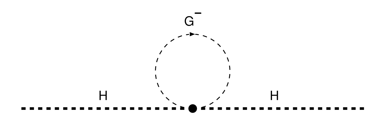
Figure 1: One of the tadpole diagrams for the Higgs self-energy

Finally, it is worth mentioning that for the $W^{\pm}$ self-energy, the calculations are more complicated, specially because there is now a richer tensorial structure involved since we have three independent vectors to our disposal namely $u^{\mu}$, $q^{\mu}$ and $b^{\mu}$. Therefore, these self-energies can be written as a linear combination of nine independent structures  D’Olivo et al. (2003). In our case, only $u^{\mu}$ and $b^{\mu}$ remain since we are considering the IR limit. So, in this limit the structure of the self-energy, collapses to $\Pi^{\mu\nu}_{ab}=\Pi^{Q}_{ab}Q^{\mu\nu}+\Pi^{R}_{ab}R^{\mu\nu}+\Pi^{S}_{ab}S^{\mu\nu}+\Pi^{M}_{ab}g^{\mu\nu}$ where $Q^{\mu\nu}=u^{\mu}u^{\nu},S^{\mu\nu}=u^{\mu}b^{\nu}+u^{\nu}b^{\mu},R^{\mu\nu}=b^{\mu}b^{\nu}$ and the transversality condition $q_{\mu}\Pi_{ab}^{\mu\nu}=0$ is trivially satisfied. For further details on this result, please refer to  Navarro et al. (2008); Navarro (2008). We perform several checks on our calculations and it is worth emphasizing that, in the limit of zero external magnetic field, we recover results already reported in literature  Carrington (1992). Moreover it is well known that in the absence of an external magnetic fields, the MSM thermal self-energies are gauge independent when considering only the leading contributions in temperature Le Bellac (1996). However, when considering the effects of a weak external magnetic field, these self-energies turn out to be gauge dependent.

4 Final remarks

During this talk we work with the degrees of freedom in the broken symmetry phase of the MSM to analyze the development of the EWPT in the presence of a weak magnetic field. We calculate the particle self-energies that include the effects of the external field. Still in progress is the ${\mathcal{O}}[(eB)^{2}]$ contribution to the effective potential, adding the ring corrections and the numerical analysis of its behavior near the phase transition. Finally, a study on gauge dependence of the effective potential is crucial for further developments.

Acknowledgments: The research discussed in this talk is partially supported by Intercambio UNAM-USON under grant PZ-444, DGAPA under grant PAPIIT IN116008, CONACyT under grants 52547-F and 40025-F and Universidad del Atlántico.

References

- Sakharov (1967) A. D. Sakharov, Pisma Zh. Eksp. Teor. Fiz. 5, 32–35 (1967).
- Yao et al. (2006) W. M. Yao, et al., J. Phys. G33, 1–1232 (2006).
- Kronberg (1994) P. P. Kronberg, Rept. Prog. Phys. 57, 325–382 (1994).
- Beck and et al (1996) R. Beck, and et al, Ann. Rev. Astron. Astrophys. 34, 155–206 (1996).
- Carilli and Taylor (2002) C. L. Carilli, and G. B. Taylor, Ann. Rev. Astron. Astrophys. 40, 319–348 (2002).
- Barrow et al. (1997) J. D. Barrow, P. G. Ferreira, and J. Silk, Phys. Rev. Lett. 78, 3610–3613 (1997).
- Sanchez et al. (2007) A. Sanchez, A. Ayala, and G. Piccinelli, Phys. Rev. D75, 043004 (2007).
- Ayala et al. (2005) A. Ayala, A. Sanchez, G. Piccinelli, and S. Sahu, Phys. Rev. D71, 023004 (2005).
- Piccinelli and Ayala (2004) G. Piccinelli, and A. Ayala, Lect. Notes Phys. 646, 293–308 (2004).
- Giovannini and Shaposhnikov (1998) M. Giovannini, and M. E. Shaposhnikov, Phys. Rev. D57, 2186–2206 (1998).
- Elmfors et al. (1998) P. Elmfors, K. Enqvist, and K. Kainulainen, Phys. Lett. B440, 269–274 (1998).
- Kajantie and et al (1999) K. Kajantie, and et al, Nucl. Phys. B544, 357–373 (1999).
- Navarro et al. (2008) J. Navarro, M. E. Tejeda-Yeomans, A. Sanchez, G. Piccinelli, and A. Ayala (2008), work in progress.
- Schwinger (1951) J. S. Schwinger, Phys. Rev. 82, 914–927 (1951).
- Erdas et al. (1998) A. Erdas, C. W. Kim, and T. H. Lee, Phys. Rev. D58, 085016 (1998).
- Chyi et al. (2000) T.-K. Chyi, et al., Phys. Rev. D62, 105014 (2000).
- D’Olivo et al. (2003) J. C. D’Olivo, J. F. Nieves, and S. Sahu, Phys. Rev. D67, 025018 (2003).
- Maartens (2000) R. Maartens, Pramana 55, 575–583 (2000).
- Ambjorn and Olesen (1989) J. Ambjorn, and P. Olesen, Nucl. Phys. B315, 606 (1989).
- Bedingham (2000) D. J. Bedingham (2000), hep-ph/0011012.
- Weldon (1993) H. A. Weldon, Phys. Rev. D47, 594–600 (1993).
- Ayala et al. (2008) A. Ayala, G. Piccinelli, A. Sanchez, and M. Tejeda-Yeomans (2008), work in progress.
- Aoki and et al (1982) K. I. Aoki, and et al, Prog. Theor. Phys. Suppl. 73, 1–225 (1982).
- Tentyukov and Fleischer (2000) M. Tentyukov, and J. Fleischer, Comput. Phys. Commun. 132, 124–141 (2000).
- Navarro (2008) J. Navarro (2008), ph.D. thesis, in progress.
- Carrington (1992) M. E. Carrington, Phys. Rev. D45, 2933–2944 (1992).
- Le Bellac (1996) M. Le Bellac (1996), Cambridge University Press.