Scaling in the distribution of intertrade durations of Chinese stocks

Abstract

The distribution of intertrade durations, defined as the waiting times between two consecutive transactions, is investigated based upon the limit order book data of 23 liquid Chinese stocks listed on the Shenzhen Stock Exchange in the whole year 2003. A scaling pattern is observed in the distributions of intertrade durations, where the empirical density functions of the normalized intertrade durations of all 23 stocks collapse onto a single curve. The scaling pattern is also observed in the intertrade duration distributions for filled and partially filled trades and in the conditional distributions. The ensemble distributions for all stocks are modeled by the Weibull and the Tsallis $q$-exponential distributions. Maximum likelihood estimation shows that the Weibull distribution outperforms the $q$-exponential for not-too-large intertrade durations which account for more than 98.5% of the data. Alternatively, nonlinear least-squares estimation selects the $q$-exponential as a better model, in which the optimization is conducted on the distance between empirical and theoretical values of the logarithmic probability densities. The distribution of intertrade durations is Weibull followed by a power-law tail with an asymptotic tail exponent close to 3.

, ,

1 Introduction

Intertrade duration is the waiting time between consecutive transactions of an equity, which contains information contents of trading activity and has crucial relevance to the microstructure theory Diamond-Verrecchia-1987-JFE , Easley-OHara-1992-JF , Dufour-Engle-2000-JF . The intertrade duration is a measure of trade intensity, which is associated with price adjustments. Short intertrade durations lead to large price change and long intertrade durations minimize the price impact in a transaction Jasiak-1999-Finance . The order placement process in stock market can be treated as a point process. Based on estimating event intensity of the marked point process, an autoregressive conditional duration (ACD) model is proposed by Engle and Russell for modeling trade duration with temporal correlation and other financial variables Engle-Russell-1998-Em , Engle-2000-Em . In this framework, the intertrade duration $\tau$ is modeled as follows

$$\tau=\psi\epsilon~{},$$ (1)

where $\psi$ is the expected value of $\tau$ and $\epsilon$ is an independent and identically distributed variable, known as the normalized duration. There are variants of the ACD model, such as the fractional integrated ACD model Jasiak-1999-Finance , the logarithmic ACD model Bauwens-Giot-2000-AES , the threshold autoregressive conditional duration (TACD) model Zhang-Russell-Tsay-2001-JEm , the stochastic conditional duration (SCD) model Bauwens-Veredas-2004-JEm , and the stochastic volatility duration (SVD) model Ghysels-Gourieroux-Jasiak-2004-JEm . In the model specification, there are different assumptions for the distribution of normalized duration, such as exponential, Weibull, generalized Gamma, Burr Sun-Rachev-Fabozzi-Kalev-2008-AF . We note that the Burr XII distribution is a general form of the Tsallis $q$-exponential distribution Burr-1942-AMS , Tsallis-1988-JSP , Nadarajah-Kotz-2006-PLA .

Alternatively, in the econophysics community, the continuous-time random walk (CTRW) formulism has been adopted to deal with the intertrade durations and price dynamics Scalas-Gorenflo-Mainardi-2000-PA , Mainardi-Raberto-Gorenflo-Scalas-2000-PA , Masoliver-Montero-Weiss-2003-PRE , Scalas-2006-PA , Masoliver-Montero-Perello-Weiss-2006-JEBO . By analogy with diffusion, the variations of log prices (or zero-mean returns) and the associated time intervals are considered as jump steps and waiting times between consecutive steps in CTRW processes. According to the CTRW formulism, the probability density function $p(X,t)$ can be expressed as follows,

$$p(X,t)=\delta(X)C(t)+\int^{t}_{0}{\rm d}t^{\prime}f(t-t^{\prime})\int^{+\infty}_{-\infty}{\rm d}x^{\prime}\lambda(X-X^{\prime})p(X^{\prime},t^{\prime})~{},$$ (2)

where $X$ represents the log prices or zero-mean returns, $C(t)$ is the complementary cumulative function (or survival probability function), and $f(t)$ is the probability density function. As shown in Eq. (2), finding $C(t)$ is a key step for obtaining the expression of $p(X,t)$. By assuming that jump steps and waiting times are uncorrelated, the complementary cumulative distribution can be theoretically approximated by the Mattag-Leffler function Scalas-Gorenflo-Mainardi-2000-PA , Mainardi-Raberto-Gorenflo-Scalas-2000-PA ,

$$C(\tau)=E_{\beta}[-(\tau/\tau_{0})^{\beta}]:=\sum_{n=0}^{\infty}(-1)^{n}\frac{[-(\tau/\tau_{0})^{\beta}]^{n}}{\Gamma(\beta n+1)},~{}~{}\beta>0.$$ (3)

Note that Eq. (3) has already been verified in some empirical studies, such as the waiting time distribution of BUND futures traded on the LIFFE Mainardi-Raberto-Gorenflo-Scalas-2000-PA and 10 stocks traded in the Irish stock market Sabatelli-Keating-Dudley-Richmond-2002-EPJB . If $\beta=1$ in Eq. (3), the Mattag-Leffler function reduces to a simple exponential function. If $0<\beta<1$, it bridges a stretched exponential and a power law Raberto-Scalas-Mainardi-2002-PA

$$E_{\beta}[-(\tau/\tau_{0})^{\beta}]\sim\left\{\begin{aligned} \exp[-(\tau/\tau_{0})^{\beta}/\Gamma(1+\beta)],~{}~{}&~{}~{}\tau/\tau_{0}\rightarrow 0^{+},\\ (\tau/\tau_{0})^{-\beta}/\Gamma(1-\beta),~{}~{}&~{}~{}\tau/\tau_{0}\rightarrow\infty.\end{aligned}\right.$$ (4)

Empirical analysis of waiting times for different financial data unveils that the probability distribution can also be described by power laws Sabatelli-Keating-Dudley-Richmond-2002-EPJB , Yoon-Choi-Lee-Yum-Kim-2006-PA , modified power laws Masoliver-Montero-Weiss-2003-PRE , Masoliver-Montero-Perello-Weiss-2006-JEBO , stretched exponentials (or Weibulls) Bartiromo-2004-PRE , Raberto-Scalas-Mainardi-2002-PA , Ivanov-Yuen-Podobnik-Lee-2004-PRE , Sazuka-2007-PA , stretched exponentials followed by power laws Kim-Yoon-2003-Fractals , Kim-Yoon-Kim-Lee-Scalas-2007-JKPS , to list a few. In a recent paper, by rejecting the hypothesis that the waiting time distributions are described by an exponential Scalas-Gorenflo-Luckock-Mainardi-Mantelli-Raberto-2004-QF , Scalas-Gorenflo-Luckock-Mainardi-Mantelli-Raberto-2005-FL or a power law Poloti-Scalas-2008-PA , Politi and Scalas reported that both Weibull distribution and $q$-exponential distribution can be utilized to approximate the intertrade duration distribution Poloti-Scalas-2008-PA . In their empirical investigation, Politi and Scalas found that the $q$-exponential compares well to the Weibull. They also argued that the distribution differing from an exponential is the consequence of the varying transaction activities during the trading period Scalas-Gorenflo-Luckock-Mainardi-Mantelli-Raberto-2004-QF , Poloti-Scalas-2008-PA , Scalas-Gorenflo-Luckock-Mainardi-Mantelli-Raberto-2005-FL , Scalas-Kaizoji-Kirchler-Huber-Tedeschi-2006-PA , Politi-Scalas-2007-PA . All this empirical evidence shows that the transaction dynamics can not be modeled by the Poisson process, rejecting the exponential distribution of intertrade durations.

An interesting feature can be observed in the empirical results of Politi and Scalas Poloti-Scalas-2008-PA . They have investigated the Trade and Quotes data set of 30 stocks, constituents of the DJIA index, traded on the NYSE in October 1999. The estimated parameters of the Weibull and $q$-exponential seem close across different stocks. This observation suggests the possible presence of scaling in the intertrade duration distributions of different stocks. Such common scaling pattern was reported for the 30 DJIA stocks over a period of four years from January 1993 till December 1996 Ivanov-Yuen-Podobnik-Lee-2004-PRE . The scaling behavior underpins common underlying dynamics between different stocks and has important implications for stock modeling. In contrast, Eisler and Kertész analyzed about 4000 stocks and found that the scaling was not convincing Eisler-Kertesz-2006-EPJB . Specifically, they divided the stocks into two groups based on the average intertrade duration of individual stocks and performed an extended self-similarity (ESS) analysis for each group of data, which resulted in a nonlinear ESS exponent function with respect to the order. This conclusion seems quite sound since a marked discrepancy between the tails can be observed in both studies Ivanov-Yuen-Podobnik-Lee-2004-PRE , Eisler-Kertesz-2006-EPJB . In this work, we shall show that such scaling in intertrade duration distributions holds for Chinese stocks and the functional form of the distribution can also be modeled by the Weibull, as reported in the DJIA stocks Ivanov-Yuen-Podobnik-Lee-2004-PRE . No obvious discrepancy between the duration distributions is observed in the Chinese stocks, in contrast to the USA stocks.

This paper is organized as follows. In Section 2, we briefly describe the data sets analyzed. Section 3 investigates the scaling behavior of the unconditional distribution of intertrade durations. We will fit the corresponding distribution by means of Weibull distribution and $q$-exponential distribution. Section 4 studies the conditional distribution of intertrade durations. Section 5 concludes.

2 Data sets

The study is based on the data of the limit-order books of 23 liquid Chinese stocks listed on the Shenzhen Stock Exchange (SZSE) in the whole year 2003. The limit-order book records ultra-high-frequency data whose time stamps are accurate to 0.01 second including details of every event (order placement and cancelation). There were three time periods on each trading day in the SZSE before July 1, 2006, named the open call action (9:15 am to 9:25 am), the cooling period (9:25 am to 9:30 am), and the continuous double auction (9:30 am to 11:30 am and 13:00 pm to 15:00 pm). During the period of open call auction, all the incoming orders are executed based on the maximal transaction volume principle at 9:25 am. In the cooling period, all orders are allowed to add into limit-order book, but no one is executed. Only in the period of continuous auction, transaction occurs based on one by one matching of incoming effective market orders and limit orders waiting on the limit-order book. Therefore, only trades during the continuous double auction are considered. In addition, we stress that no intertrade duration is calculated between two trades overnight or crossing the noon closing. Assuming that there are $n$ trades at times $\{t_{i}:i=1,2,\cdots,n\}$ during the time interval from 9:30 am to 11:30 am or from 13:00 pm to 15:00 pm on a trading day, we obtain $n-1$ intertrade durations $\tau_{i}=t_{i+1}-t_{i}$ with $i=1,2,\cdots,n-1$.

In 2003, only limit orders are allowed for submission in the Chinese stock market and the tick size of all stocks is one cent of Renminbi (the Chinese currency). Those orders resulting in immediate execution, whose prices are equal to or higher than the best ask price for buys and equal to or lower than the best bid price for sells, can be called as effective market orders. Effective market orders can be classified into two types based on their aggressiveness, namely filled effective market orders and partially filled effective market orders. Partially filled orders are more aggressive than filled orders since the former have much larger price impact Zhou-2007-XXX . The trades can be classified into two types accordingly, called filled trades and partially filled trades for brevity that are initiated respectively by filled and partially filled effective market orders. We will consider two additional classes of durations, involving $\tau_{\rm{F}}$ between two consecutive filled trades and $\tau_{\rm{PF}}$ between two successive partially filled trades. Table 1 provides the number of trades and average intertrade duration for the 23 Chinese stocks under investigation for all trades, filled trades, and partial filled trades. We find that $\langle\tau_{\rm{F}}\rangle\ll\langle\tau_{\rm{PF}}\rangle$ and $N_{\rm{PF}}\ll N_{\rm{F}}$, since $N_{\rm{F}}\langle\tau_{\rm{F}}\rangle\approx N_{\rm{PF}}\langle\tau_{\rm{PF}}\rangle$. Although the time resolution of our data is as precise as 0.01 second, there are still trades stamped with the same time. In Table 1, we also presents the numbers of vanishing intertrade durations for the three types of trades. We see that their proportions are relatively low. More information about the SZSE trading rules and the data sets can be found in Refs. Gu-Chen-Zhou-2007-EPJB , Gu-Chen-Zhou-2008a-PA , Gu-Chen-Zhou-2008b-PA .

Table 1: The number of trades, the number of vanishing intertrade durations and average intertrade duration for the 23 Chinese stocks

Code		All trades				Filled trades				Partly filled trades
		$N$	$N^{0}$	$\langle\tau\rangle$		$N_{\rm{F}}$	$N^{0}_{\rm{F}}$	$\langle\tau_{\rm{F}}\rangle$		$N_{\rm{PF}}$	$N^{0}_{\rm{PF}}$	$\langle\tau_{\rm{PF}}\rangle$
000001		889369	17809	3.81		823603	16184	4.11		65766	69	51.27
000002		509361	10922	6.69		476457	10380	7.14		32904	20	101.86
000009		447968	5628	7.69		413531	5185	8.33		34437	17	98.91
000012		290381	2092	11.69		250078	1763	13.56		40303	24	83.39
000016		188613	1513	18.14		159497	1324	21.43		29116	10	116.32
000021		411642	4468	8.33		360503	3972	9.50		51139	26	66.63
000024		133587	1815	25.13		111691	1675	30.00		21896	6	150.81
000027		313898	8908	10.83		288205	8457	11.79		25693	13	128.31
000063		265479	9754	12.76		237957	9380	14.22		27522	8	120.42
000066		277654	2329	12.32		240016	2063	14.24		37638	15	89.92
000088		97196	7060	34.87		84183	6856	40.15		13013	12	250.16
000089		189118	5097	17.88		168599	4728	20.04		20519	9	160.85
000406		271390	3181	12.66		237390	2880	14.46		34000	11	100.36
000429		117425	564	28.79		101329	496	33.30		16096	3	204.91
000488		120098	1294	28.32		95015	1158	35.76		25083	5	134.35
000539		114722	15245	29.27		98296	14812	34.10		16426	15	199.73
000541		68738	666	49.35		56232	599	60.22		12506	0	262.69
000550		346710	9331	9.88		305386	8760	11.21		41324	22	82.03
000581		93976	4471	35.79		77748	4192	43.12		16228	5	200.46
000625		397566	9438	8.43		350333	8645	9.56		47233	36	70.44
000709		207816	3676	16.39		187431	3461	18.16		20385	6	163.59
000720		132243	17195	25.42		110699	14455	30.35		21544	1	152.39
000778		157322	1527	21.6		133944	1318	25.33		23378	5	143.16

3 Unconditional distributions of intertrade durations

3.1 Scaling pattern

For each stock, the three groups of durations $\tau$, $\tau_{\rm{F}}$ and $\tau_{\rm{PF}}$ (in units of second) are calculated for all trades, filled trades and partially filled trades. The associated empirical density functions $f(\tau)$, $f(\tau_{\rm{F}})$ and $f(\tau_{\rm{PF}})$ for the 23 Chinese stocks are illustrated in the upper panel of Fig. 1. At a first glance, we observe that different distributions share similar shapes. When the duration is large, the tails are heavy but it is not unambiguous that they exhibit power-law tails. Since the time stamps of the data have a resolution of 0.01 second, the minimal duration is set to be 0.01 in the plots. There are also vanishing durations as shown in Table 1, which are not shown in this figure. Note that the density functions are monotonically decreasing such that small durations occur more frequent than large ones.

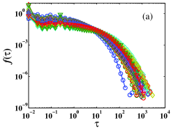
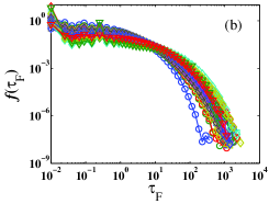
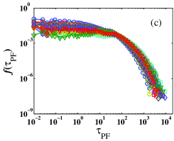
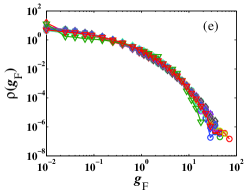
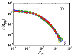
Figure 1: (Color online.) Scaling in the unconditional distributions of 23 stocks. Panels (a-c) illustrate the empirical density functions of intertrade durations for all trades, filled trades and partially filled trades. Panels (d-f) present the empirical density functions of the normalized intertrade durations for all trades, filled trades and partially filled trades.

In order to compare the distributions of different stocks, we define a normalized duration by

$$g=\tau/{\sigma},~{}g_{\rm{F}}=\tau_{\rm{F}}/{\sigma_{\rm{F}}},~{}g_{\rm{PF}}=\tau_{\rm{PF}}/{\sigma}_{\rm{PF}},$$ (5)

where $\sigma$, $\sigma_{\rm{F}}$ and $\sigma_{\rm{PF}}$ are the sample standard deviations of $\tau$, $\tau_{\rm{F}}$ and $\tau_{\rm{PF}}$, respectively. As will be clear, the variances $\sigma^{2}$, $\sigma_{\rm{F}}^{2}$ and $\sigma_{\rm{PF}}^{2}$ of intertrade durations exist for the Chinese stocks. Then the PDFs of these normalized durations can be obtained as follows,

$$\rho(g)=\sigma f(g\sigma),~{}\rho(g_{\rm{F}})=\sigma_{\rm{F}}f(g\sigma_{\rm{F}}),~{}\rho(g_{\rm{PF}})=\sigma_{\rm{PF}}f(g\sigma_{\rm{PF}}).$$ (6)

In the lower panel of Fig. 1, we plot respectively $\sigma f(\tau)$, $\sigma_{\rm{F}}f(\tau_{\rm{F}})$ and $\sigma_{\rm{PF}}f(\tau_{\rm{PF}})$ as functions of $\tau/{\sigma}$, $\tau_{\rm{F}}/{\sigma_{\rm{F}}}$ and $\tau_{\rm{PF}}/{\sigma}_{\rm{PF}}$ for the 23 stocks. In each plot, the 23 curves excellently collapse onto a single curve. We notice that the collapsing for the Chinese stocks is better than those DJIA stocks, especially for large values of the normalized durations Ivanov-Yuen-Podobnik-Lee-2004-PRE . This analysis shows that $\rho(g)$, $\rho(g_{\rm{F}})$ and $\rho(g_{\rm{PF}})$ are scaling functions.

3.2 Fitting the intertrade duration distributions

The nice scaling in the distribution of intertrade durations means that the normalized durations of different stocks follow the same distribution. This allows us to treat all the normalized intertrade durations from different stocks as an ensemble to gain better statistics. In this way, we have three aggregate samples for $g$, $g_{\rm{F}}$ and $g_{\rm{PF}}$. The three empirical probability density functions of the three types of normalized intertrade durations are illustrated in Fig. 2 as dots.

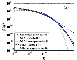
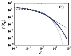
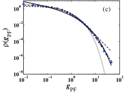
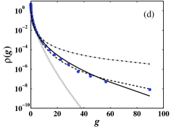
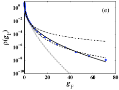
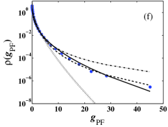
Figure 2: (Color online.) Empirical probability density function of normalized intertrade durations as an ensemble of the 23 stocks. The solid and dashed lines are the least square nonlinear fits of the Weibull and $q$-exponential distributions. The dotted and dash-dotted lines are the maximum likelihood fits to the Weibull and $q$-exponential distributions. The upper panel shows double logarithmic plots, while the lower panel shows semi-logarithmic plots for comparison.

Following the work of Politi and Scalas Poloti-Scalas-2008-PA , we adopt the Weibull and the $q$-exponential distributions to model the normalized intertrade durations. The Weibull probability density $\rho_{w}(g)$ can be written as

$$\rho_{w}(g)=\alpha\beta g^{\beta-1}\exp(-\alpha g^{\beta}),$$ (7)

and its complementary (cumulative) distribution function $C_{w}(g)$ is

$$C_{w}(g)=\exp(-\alpha g^{\beta}).$$ (8)

When $\beta=1$, $\rho_{w}(g)$ recovers the exponential distribution. When $0<\beta<1$, $\rho_{w}(g)$ is a stretched exponential or sub-exponential. When $\beta>1$, $\rho_{w}(g)$ is a super-exponential. The $q$-exponential probability density $\rho_{q}(g)$ is defined by

$$\rho_{q}(g)=\mu\left[1+(1-q)(-\mu g)\right]^{\frac{q}{1-q}},$$ (9)

and its complementary cumulative distribution function $C_{q}(\tau)$ is

$$C_{q}(g)=\left[1+(1-q)(-\mu g)\right]^{\frac{1}{1-q}}.$$ (10)

Usually, we have $q>1$. When $(1-q)(-\mu g)\gg 1$, we observe a power-law behavior in the tail $C_{q}(g)\sim g^{-{1}/{(q-1)}}$ with a tail exponent of $1/(q-1)$.

In order to capture the main part of the distributions, we adopt the maximum likelihood estimator (MLE) for model calibration. Specifically, the MATLAB function “wblfit” is utilized to estimate the parameters of the Weibull and the estimation method for the $q$-exponential can be found in Ref. Shalizi-2007-XXX . The resultant fits are illustrated in Fig. 2. It is evident that both distributions fit the data very well for the normalized durations less than about 4, which accounts for 98.5% of the sample. However, there are remarkable discrepancies in the tails between the empirical data and the two models. Table 2 reports the estimates of parameters. Since both Weibull and $q$-exponential models have two parameters, we can compare quantitatively their performance simply using the r.m.s. values of fit residuals. According to Table 2, the Weibull model outperforms the $q$-exponential model since $\chi_{w}<\chi_{q}$.

Table 2: Estimated values of parameters ($\alpha$, $\beta$, $q$, $\mu$) by means of MLE. $\chi_{w}$ and $\chi_{q}$ stand for the r.m.s. of fit residuals. The $p$ value in parentheses represents the percentage of stocks preferring the chosen model in the column.

Duration		Weibull				$q$-exponential
		$\alpha$	$\beta$	$\chi_{w}$, ($p$)		$\mu$	$q$	$\chi_{q}$, ($p$)
$g$		1.85	0.68	0.71		4.17	1.65	1.35
mean $\pm$ std		$1.85\pm 0.15$	$0.69\pm 0.03$	(19/23)		$4.18\pm 0.99$	$1.63\pm 0.09$	(4/23)
$g_{\rm{F}}$		1.90	0.67	0.93		4.60	1.69	1.57
mean $\pm$ std		$1.90\pm 0.16$	$0.67\pm 0.03$	(19/23)		$4.64\pm 1.19$	$1.68\pm 0.10$	(4/23)
$g_{\rm{PF}}$		1.71	0.74	0.10		2.96	1.46	1.09
mean $\pm$ std		$1.73\pm 0.15$	$0.74\pm 0.04$	(14/23)		$3.12\pm 0.74$	$1.47\pm 0.10$	(9/23)

We have also fitted the distributions for individual stocks (see the three tables in Appendix of the paper at http://arXiv.org/abs/0804.3431). For individual stocks, the Weibull model also outperforms the $q$-exponential model. The parameters, especially $\beta$ and $q$, are consistent across different stocks. The mean and standard deviation for each case are also calculated and listed in Table 2. We find that, for each type of intertrade durations, the corresponding parameters estimated from the ensemble and individual stocks are close to one another. For the case of $g$ (and $g_{\rm{F}}$) as well, there are 19 stocks (out of 23) prefer the Weibull model in the sense that $\chi_{w}<\chi_{q}$. For $g_{\rm{PF}}$, 14 stocks prefer the Weibull distribution and 9 stocks prefer the $q$-exponential model. Therefore, the $q$-exponential is still a good model for the bulk distribution of durations.

In order to capture the tail behavior of the distributions, we adopt the nonlinear least square estimator (NLSE) for model calibration. Specifically, the MATLAB function “lsqcurvefit” is utilized to estimate the parameters of the two models. The objective function in the fitting is $\sum[\ln\rho(g)-\ln\hat{\rho}(g)]^{2}$ rather than $\sum[\rho(g)-\hat{\rho}(g)]^{2}$, where $\hat{\rho}(g)$ is the empirical data. The resultant fits are also illustrated in Fig. 2 and Table 3 reports the estimates of parameters. It is evident from Fig. 2 that the $q$-exponential is a better model than the Weibull except $g_{\rm{F}}$, which is confirmed by the much smaller values of $\chi_{q}$ compared with $\chi_{w}$ in Table 3. The fact that the tail distributions can be better modeled by the $q$-exponential implies that the intertrade durations have a power-law tail distribution. The estimated tail exponents are 4.00, 4.17 and 3.70 for $g$, $g_{\rm{F}}$ and $g_{\rm{PF}}$.

Table 3: Estimated values of parameters ($\alpha$, $\beta$, $q$, $\mu$) by means of NLSE. $\chi_{w}$ and $\chi_{q}$ stand for the r.m.s. of fitting residuals. The $p$ value in parentheses represents the percentage of stocks preferring the chosen model in the column.

Duration		Weibull				$q$-exponential
		$\alpha$	$\beta$	$\chi_{w}$, ($p$)		$\mu$	$q$	$\chi_{q}$,( $p$)
$g$		2.24	0.46	22.41		1.99	1.25	17.02
mean $\pm$ std		$2.10\pm 0.14$	$0.49\pm 0.03$	(9/23)		$2.38\pm 0.29$	$1.30\pm 0.03$	(14/23)
$g_{\rm{F}}$		2.12	0.48	12.44		1.93	1.24	23.03
mean $\pm$ std		$2.18\pm 0.14$	$0.47\pm 0.04$	(11/23)		$2.51\pm 0.38$	$1.31\pm 0.04$	(12/23)
$g_{\rm{PF}}$		1.96	0.52	19.26		2.07	1.27	4.81
mean $\pm$ std		$2.00\pm 0.14$	$0.50\pm 0.04$	(2/23)		$2.64\pm 0.41$	$1.36\pm 0.04$	(21/23)

Similarly, we have also fitted the distributions for individual stocks using NLSE (see the three tables in Appendix of the paper at http://arXiv.org/abs/0804.3431). For more than a half of the stocks, the $q$-exponential model also outperforms the Weibull model. The parameters, especially $\beta$ and $q$, are consistent across different stocks. The mean and standard deviation for each case are also calculated and listed in Table 3. We find that, for each type of intertrade durations, the corresponding parameters estimated from the ensemble and individual stocks are close to one another. The tail exponents for $g$, $g_{\rm{F}}$ and $g_{\rm{PF}}$ are estimated to be 3.33, 3.23, and 2.78, which is reminiscent of the inverse cubic law of returns at microscopic timescale Gopikrishnan-Meyer-Amaral-Stanley-1998-EPJB , Gu-Chen-Zhou-2008a-PA .

4 Conditional distributions of intertrade durations

We now investigate the conditional distribution of normalized intertrade durations on the value of its preceding duration. All the normalized durations for different stocks constitute an ensemble set $Q$, which is partitioned into five non-overlapping groups:

$$Q=Q_{1}\cup Q_{2}\cup Q_{3}\cup Q_{4}\cup Q_{5}~{},$$ (11)

where $Q_{i}\cap Q_{j}=\phi$ for $i\neq j$. In the partitioning procedure, all values in $Q$ are sorted in increasing order and assigned into $Q_{1}$ to $Q_{5}$ such that their sizes are approximately identical. We estimate the empirical conditional probability density functions $p(g|g_{0})$ of normalized intertrade durations that immediately follow a normalized intertrade duration $g_{0}$ belonging to $Q_{i}$. The five empirical conditional PDFs are depicted in Fig. 3(a). Again, all the five PDFs collapse onto a single curve, showing a nice scaling relation in the conditional distributions of intertrade durations. Comparing with Fig. 2, we see that $p(g|g_{0})\approx\rho(g)$.

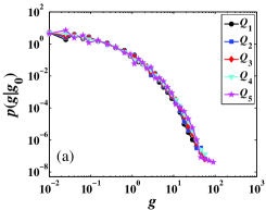
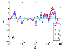
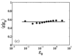
Figure 3: (Color online.) Scaling in the conditional distributions of intertrade durations. (a) Conditional probability distribution $p(g|g_{0})$ with respect to $g$. (b) Plots of $z_{i}=\ln[p(g|Q_{5})/p(g|Q_{i})]$ for $i=1$ to 4. (c) Mean conditional duration $\langle g|g_{0}\rangle$ with respect to $g_{0}$.

However, a careful scrutiny of Fig. 3(a) unveils a systematic trend in the five conditional PDFs identifying that, in the tails, the PDF for $Q_{1}$ is on the bottom while that for $Q_{5}$ lies on the top. It means that there are more large durations for $Q_{i}$ than $Q_{j}$ if $i>j$. Speaking differently, large durations tend to follow large durations. To further clarify this observation, we plot $z_{i}=\ln[p(g|Q_{5})/p(g|Q_{i})]$ for $i=1$ to 4 in Fig. 3(b). It is clear that the five PDFs deviate from one another systematically for large $g$. The discrepancy is much weaker for small $g$. This phenomenon can also be confirmed by the mean conditional duration $\langle g|g_{0}\rangle$. If $p(g|g_{0})=\rho(g)$, we will have

$$\langle g|g_{0}\rangle=\int_{0}^{\infty}p(g|g_{0})g{\rm{d}}g=\int_{0}^{\infty}\rho(g)g{\rm{d}}g=\langle g\rangle~{}.$$ (12)

In other words, the mean conditional duration $\langle g|g_{0}\rangle$ is independent of $g_{0}$. Fig. 3(c) plots the mean conditional duration $\langle g|g_{0}\rangle$ against $g_{0}$. When $g_{0}$ is not too small, we see an upward trend in $\langle g|g_{0}\rangle$ with respect to $g_{0}$. However, the $\langle g|g_{0}\rangle$ values are still close to $\langle g\rangle$, indicated by the horizontal line in Fig. 3(c).

5 Conclusion

We have investigated the intertrade durations calculated from the limit order book data of 23 liquid Chinese stocks traded on the SZSE in the whole year 2003. The density functions are found to be monotonically decreasing with respect to increasing intertrade duration. After normalized by the stock-dependent standard deviation of intertrade durations, the 23 empirical distributions of durations collapse onto a single curve, indicating a nice scaling pattern. This scaling behavior is also observed in the distributions of waiting times between consecutive filled trades or partially filled trades. Therefore, we can treat the normalized intertrade durations of different stocks as realizations of an ensemble. The scaling pattern implies that there are common features in the trading behavior of market participants, which also has important implications for market microstructure theory.

The three ensemble distributions of normalized intertrade durations for all trades, filled trades and partially filled trades are modeled by the Weibull and the Tsallis $q$-exponential using maximum likelihood estimator and nonlinear least-squares estimator. We find that more than 98.5% of the intertrade durations can be well modeled by the Weibull function using MLE, except for the tails, and the logarithmic density functions can be better fitted by the $q$-exponential function utilizing NLSE. By and large, the intertrade duration distribution has a Weibull form followed by a power-law tail for large durations. We also studied the conditional distribution of normalized intertrade durations that immediately follow a normalized intertrade duration. A scaling pattern is also observed in these conditional distributions decorated with a weak but systematic trend. Accordingly, the mean conditional intertrade duration is weakly dependent on the preceding intertrade duration.

Acknowledgments:

We are grateful to Z. Eisler for discussion. This work was partially supported by the National Natural Science Foundation of China (Nos. 70501011 and 70502007), the Fok Ying Tong Education Foundation (No. 101086), the Shanghai Rising-Star Program (No. 06QA14015), and the Program for New Century Excellent Talents in University (No. NCET-07-0288).

Appendix A Fitted parameters for the three classes of intertrade durations

Table 4: Values of fitted parameters, $\alpha$, $\beta$ $q$, $\mu$ for the distribution of 23 stocks for all trades duration.

Stock code	MLE							NLSE
	$\alpha$	$\beta$	$\chi_{w}$	$\mu$	$q$	$\chi_{q}$		$\alpha$	$\beta$	$\chi_{w}$	$\mu$	$q$	$\chi_{q}$
000001	1.69	0.71	1.04	3.30	1.57	1.11		2.15	0.49	27.17	1.99	1.24	8.67
000002	1.89	0.68	0.89	4.41	1.67	1.08		2.01	0.51	10.11	2.17	1.27	16.18
000009	1.84	0.69	0.57	3.95	1.61	1.25		2.42	0.41	35.64	2.58	1.32	8.12
000012	2.14	0.66	2.09	5.72	1.70	0.57		2.44	0.40	25.37	3.12	1.38	14.96
000016	1.63	0.73	0.38	2.88	1.50	1.00		2.38	0.42	50.14	2.38	1.30	2.85
000021	1.88	0.68	1.14	4.34	1.66	1.40		2.07	0.49	12.97	2.34	1.29	14.54
000024	1.89	0.70	0.65	4.00	1.59	0.95		2.05	0.49	16.14	2.38	1.30	9.92
000027	2.01	0.65	1.58	5.48	1.75	0.95		2.10	0.49	9.06	2.46	1.30	21.85
000063	1.87	0.68	0.83	4.20	1.64	1.08		2.03	0.50	13.23	2.38	1.31	11.85
000066	1.87	0.68	0.77	4.22	1.65	1.41		2.04	0.50	11.92	2.32	1.29	13.43
000088	1.80	0.70	0.21	3.59	1.55	1.46		2.01	0.50	16.18	2.36	1.31	7.29
000089	1.85	0.67	0.54	4.23	1.66	2.57		1.93	0.53	4.76	2.21	1.28	16.79
000406	1.76	0.72	0.46	3.37	1.53	0.87		1.99	0.51	17.43	2.09	1.26	7.68
000429	1.91	0.67	0.84	4.62	1.68	1.30		2.06	0.50	10.13	2.27	1.28	17.15
000488	1.77	0.73	0.41	3.19	1.48	0.77		1.99	0.51	20.59	2.18	1.28	5.37
000539	2.00	0.62	2.87	5.98	1.82	8.68		2.07	0.48	1.67	2.55	1.33	34.82
000541	1.63	0.74	0.19	2.77	1.46	1.01		1.98	0.51	23.16	2.05	1.27	4.04
000550	2.07	0.64	1.76	6.02	1.78	1.46		2.18	0.46	8.91	2.91	1.36	22.04
000581	1.88	0.68	0.62	4.26	1.64	1.31		2.09	0.48	14.93	2.46	1.31	11.66
000625	2.06	0.67	1.39	5.25	1.69	0.74		2.17	0.46	14.72	2.9	1.36	13.94
000709	1.86	0.68	1.05	4.28	1.66	1.31		2.09	0.49	14.62	2.37	1.30	13.29
000720	1.53	0.67	7.55	2.75	1.55	19.08		2.04	0.50	11.30	2.01	1.26	24.38
000778	1.74	0.71	0.46	3.34	1.54	0.93		2.04	0.50	21.34	2.21	1.28	6.48

Table 5: Values of fitted parameters, $\alpha$, $\beta$ $q$, $\mu$ for the distribution of 23 stocks for filled trades duration.

Stock code	MLE							NLSE
	$\alpha$	$\beta$	$\chi_{w}$	$\mu$	$q$	$\chi_{q}$		$\alpha$	$\beta$	$\chi_{w}$	$\mu$	$q$	$\chi_{q}$
000001	1.73	0.70	0.85	3.51	1.59	1.17		2.01	0.53	14.82	1.93	1.23	11.48
000002	1.94	0.67	1.02	4.80	1.69	1.21		2.03	0.51	8.65	2.25	1.28	18.92
000009	1.87	0.68	0.83	4.17	1.64	1.52		2.34	0.43	27.65	2.49	1.31	11.52
000012	2.21	0.64	3.43	6.52	1.76	0.81		2.38	0.42	18.42	2.96	1.35	25.53
000016	1.68	0.71	0.39	3.20	1.55	1.23		2.26	0.44	36.21	2.28	1.29	5.61
000021	1.95	0.66	1.44	4.93	1.71	1.46		2.30	0.44	20.13	2.61	1.32	16.78
000024	1.93	0.68	0.82	4.45	1.64	1.09		2.28	0.44	24.24	2.52	1.32	12.35
000027	2.07	0.64	1.80	6.04	1.79	1.03		2.33	0.43	15.05	2.69	1.33	23.85
000063	1.93	0.67	1.08	4.69	1.69	1.19		2.27	0.44	21.13	2.48	1.31	15.25
000066	1.93	0.66	1.18	4.77	1.70	1.50		2.31	0.44	20.41	2.44	1.30	17.45
000088	1.82	0.69	0.25	3.87	1.60	1.78		2.23	0.45	24.79	2.33	1.30	10.15
000089	1.91	0.65	1.16	4.85	1.73	3.27		2.28	0.44	14.34	2.45	1.31	21.15
000406	1.83	0.70	0.53	3.77	1.58	1.02		2.16	0.47	24.05	2.36	1.30	8.39
000429	1.96	0.65	1.12	5.12	1.73	1.49		2.24	0.46	14.71	2.61	1.32	17.81
000488	1.83	0.70	0.36	3.67	1.56	1.30		2.14	0.46	24.52	2.56	1.34	6.54
000539	2.01	0.59	4.51	6.92	1.93	10.51		2.17	0.45	1.41	2.73	1.36	43.14
000541	1.65	0.72	0.15	2.94	1.50	1.58		2.11	0.48	28.46	2.20	1.29	4.94
000550	2.15	0.62	2.68	6.93	1.84	1.54		2.21	0.46	6.67	3.48	1.41	23.27
000581	1.89	0.66	0.71	4.57	1.69	1.85		2.02	0.50	8.24	2.53	1.32	14.61
000625	2.12	0.65	1.99	5.90	1.74	0.80		2.19	0.46	12.02	3.40	1.41	14.11
000709	1.91	0.66	1.02	4.70	1.70	1.32		2.00	0.52	7.08	2.36	1.29	17.00
000720	1.51	0.66	9.53	2.77	1.59	22.33		1.90	0.55	8.26	1.83	1.22	29.66
000778	1.79	0.70	0.56	3.71	1.60	1.20		1.94	0.53	10.52	2.19	1.28	10.10

Table 6: Values of fitted parameters, $\alpha$, $\beta$ $q$, $\mu$ for the distribution of 23 stocks for partial filled trades duration.

Stock code	MLE							NLSE
	$\alpha$	$\beta$	$\chi_{w}$	$\mu$	$q$	$\chi_{q}$		$\alpha$	$\beta$	$\chi_{w}$	$\mu$	$q$	$\chi_{q}$
000001	1.68	0.70	0.56	3.17	1.55	4.84		1.78	0.58	1.83	2.21	1.29	11.34
000002	1.96	0.67	0.39	4.54	1.64	3.58		2.15	0.47	10.97	3.25	1.41	9.54
000009	1.85	0.66	0.58	4.30	1.67	4.45		2.02	0.49	7.28	2.95	1.40	11.74
000012	1.73	0.76	0.37	2.89	1.42	0.68		1.94	0.51	24.90	2.60	1.36	1.03
000016	1.48	0.80	0.11	2.09	1.33	0.49		1.78	0.54	23.38	2.10	1.31	0.48
000021	1.55	0.78	0.05	2.27	1.35	1.45		1.84	0.54	18.83	2.17	1.30	1.72
000024	1.67	0.77	0.68	2.67	1.40	0.42		1.88	0.52	26.20	2.38	1.33	0.58
000027	2.05	0.68	0.29	4.67	1.60	2.26		2.21	0.45	16.77	3.75	1.46	4.97
000063	1.81	0.75	0.65	3.17	1.45	0.34		1.98	0.51	24.39	2.66	1.35	1.06
000066	1.60	0.77	0.09	2.44	1.37	1.04		1.84	0.54	19.24	2.25	1.32	1.46
000088	1.79	0.74	1.93	3.30	1.49	0.18		1.94	0.51	27.17	2.62	1.36	0.83
000089	1.83	0.74	0.90	3.29	1.46	0.19		2.20	0.44	43.52	2.98	1.39	0.42
000406	1.54	0.79	0.11	2.26	1.35	1.01		2.04	0.47	39.77	2.35	1.34	0.84
000429	1.77	0.71	0.54	3.53	1.56	0.74		2.17	0.45	31.77	2.76	1.37	2.73
000488	1.60	0.81	1.09	2.38	1.34	0.24		2.05	0.47	53.93	2.43	1.35	0.31
000539	1.77	0.72	1.28	3.43	1.54	0.23		2.16	0.46	38.65	2.70	1.36	1.46
000541	1.59	0.79	1.24	2.45	1.38	0.33		2.05	0.47	50.28	2.35	1.33	0.28
000550	1.68	0.74	0.08	2.84	1.44	1.84		2.11	0.46	31.58	2.65	1.37	2.37
000581	1.83	0.74	1.42	3.40	1.49	0.34		2.02	0.50	28.21	2.80	1.37	0.96
000625	1.71	0.76	0.13	2.77	1.40	1.11		2.09	0.48	33.07	2.46	1.33	1.82
000709	1.81	0.70	0.15	3.71	1.58	1.72		1.96	0.52	11.35	2.61	1.35	6.20
000720	1.98	0.74	9.30	3.87	1.50	3.98		2.03	0.50	44.60	3.36	1.44	3.88
000778	1.57	0.78	0.32	2.40	1.38	0.60		1.73	0.57	14.80	2.20	1.32	0.98

References

- [1] D. W. Diamand, R. E. Verrecchia, Constraints on short-selling and asset price adjustment to private information, J. Finan. Econ. 18 (1987) 277–311.
- [2] D. Easley, M. O’Hara, Time and the process of security price adjustment, J. Finan. 47 (1992) 577–605.
- [3] A. Dufour, R. F. Engle, Time and the price impact of a trade, J. Finan. 55 (2000) 2467–2498.
- [4] J. Jasiak, Persistence in Intertrade durations, Finance 19 (1998) 166–195.
- [5] R. Engle, J. R. Russell, The Autoregressive Conditional Duration Model, Econometrica 66 (1998) 1127–1163.
- [6] R. F. Engle, The econometrics of ultra-high-frequency data, Econometrica 68 (2000) 1–20.
- [7] L. Bauwens, P. Giot, The logarithmic ACD model: An application to the bid-ask quote process of three NYSE stocks, Ann. Econ. Stat. 60 (2000) 117–149.
- [8] M. Y. J. Zhang, J. R. Russell, R. S. Tsay, A nonlinear autoregressive conditional duration model with applications to financial transaction data, J. Econometrics 104 (2001) 179–207.
- [9] L. Bauwens, D. Veredas, The stochastic conditional duration model: A latent variable model for the analysis of financial durations, J. Econometrics 119 (2004) 381–412.
- [10] E. Ghysels, C. Gourieroux, J. Jasiak, Stochastic volatility duration models, J. Econometrics 119 (2004) 413–433.
- [11] W. Sun, S. Rachev, F. J. Fabozzi, P. S. Kalev, Fractals in trade duration: capturing long-range dependence and heavy tailedness in modeling trade duration, Ann. Finan. 4 (2008) 217–241.
- [12] I. W. Burr, Cumulative frequency functions, Ann. Math. Stat. 13 (1942) 215–232.
- [13] C. Tsallis, Possible generalization of Boltzmann-Gibbs statistics, J. Stat. Phys. 52 (1988) 479–487.
- [14] S. Nadarajah, S. Kotz, exponential is a Burr distribution, Phys. Lett. A 359 (2006) 577–579.
- [15] E. Scalas, R. Gorenflo, F. Mainardi, Fractional calculus and continuous-time finance, Physica A 284 (2000) 376–384.
- [16] F. Mainardi, M. Raberto, R. Gorenflo, E. Scalas, Fractional calculus and continuous-time finance II: The waiting-time distribution, Physica A 287 (2000) 468–481.
- [17] J. Masoliver, M. Montero, G. H. Weiss, Continuous-time random walk model for financial distribution, Phys. Rev. E 67 (2003) 021112.
- [18] E. Scalas, The application of continuous-time random walks in finance and economics, Physica A 362 (2006) 225–239.
- [19] J. Masoliver, M. Montero, J. Perelló, G. H. Weiss, The continunous time random walk formalism in financial markets, J. Econ. Behav. Org. 61 (2006) 577–598.
- [20] L. Sabatelli, S. Keating, J. Dudley, P. Richmond, Waiting time distributions in financial markets, Eur. Phys. J. B 27 (2002) 273–275.
- [21] M. Raberto, E. Scalas, F. Mainardi, Waiting-times and returns in high-frequency financial data: An empirical study, Physica A 314 (2002) 749–755.
- [22] S.-M. Yoon, J. S. Choi, C. C. Lee, M.-K. Yum, K. Kim, Dynamical Volatilities for yen-dollar exchange rates, Physica A 59 (2006) 569–575.
- [23] R. Bartiromo, Dynamic of stock price, Phys. Rev. E 60 (2004) 067108.
- [24] P. C. Ivanov, A. Yuen, B. Podobnik, Y.-K. Lee, Common scaling patterns in intertrade times of U. S. stocks, Phys. Rev. E 69 (2004) 056107.
- [25] N. Sazuka, On the gap between an empirical distribution and an exponential distribution of waiting times for price changes in a financial market, Physica A 376 (2007) 500–506.
- [26] K. Kim, S.-M. Yoon, Dynamic behavior of continuous tick data in futures exchange market, Fractals 11 (2) (2003) 131–136.
- [27] K. Kim, S.-M. Yoon, S. Y. Kim, D.-I. Lee, E. Scalas, Dynamical Mechanisms of the Continuous-Time Random Walk, Multifractals,Herd Behaviors and Minority Games in Financial Markets, J. Korean Phys. Soc. 50 (2007) 182–190.
- [28] E. Scalas, R. Gorenflo, H. Luckock, F. Mainardi, M. Mantelli, M. Raberto, Anomalous waiting times in high-frequency financial data, Quant. Finance 4 (2004) 695–702.
- [29] E. Scalas, R. Gorenflo, H. Luckock, F. Mainardi, M. Mantelli, M. Raberto, On the Intertrade Waiting-time Distribution, Finan. Lett. 3 (2005) 695–702.
- [30] M. Politi, E. Scalas, Fitting the empirical distribution of intertrade durations, Physica A 387 (2008) 2025–2034.
- [31] E. Scalas, T. Kaizoji, M. Kirchler, J. Huber, A. Tedeschi, Waiting times between orders and trades in double-auction markets, Physica A 366 (2006) 463–471.
- [32] M. Politi, E. Scalas, Activity spectrum from waiting-time distribution, Physica A 383 (2007) 43–48.
- [33] Z. Eisler, J. Kertész, Size matters: Some stylized facts of the stock market revisited, Eur. Phys. J. B 51 (2006) 145–154.
- [34] W.-X. Zhou, Universal price impact functions of individual trades in an order-driven market, http://arxiv.org/abs/0708.3198v2 (2007).
- [35] G.-F. Gu, W. Chen, W.-X. Zhou, Quantifying bid-ask spreads in the Chinese stock market using limit-order book data: Intraday pattern, probability distribution, long memory, and multifractal nature, Eur. Phys. J. B 57 (2007) 81–87.
- [36] G.-F. Gu, W. Chen, W.-X. Zhou, Empirical distributions of Chinese stock returns at different microscopic timescales, Physica A 387 (2008) 495–502.
- [37] G.-F. Gu, W. Chen, W.-X. Zhou, Empirical regularities of order placement in the Chinese stock market, Physica A 387 (2008) 3173–3182.
- [38] C. R. Shalizi, Maximum Likelihood Estimation for -Exponential (Tsallis) Distributions, arXiv:math/0701854v2 (2007).
- [39] P. Gopikrishnan, M. Meyer, L. A. N. Amaral, H. E. Stanley, Inverse cubic law for the distribution of stock price variations, Eur. Phys. J. B 3 (1998) 139–140.