Characterizing symmetry breaking patterns in a lattice by dual degrees of freedom

Abstract

A duality transformation in quantum field theory is usually established first through partition functions. It is always important to explore the dual relations between various correlation functions in the transformation. Here, we explore such a dual relation to study quantum phases and phase transitions in an extended boson Hubbard model at $1/3$ ($2/3$) filling on a triangular lattice. We develop systematically a simple and effective way to use the vortex degree of freedoms on dual lattices to characterize both the density wave and valence bond symmetry breaking patterns of the boson insulating states in the direct lattices. In addition to a checkerboard charge density wave (X-CDW) and a stripe CDW, we find a novel CDW-VBS phase which has both local CDW and local valence bond solid (VBS) orders. Implications on QMC simulations are addressed. The possible experimental realizations of cold atoms loaded on optical lattices are discussed.

Various duality transformations play crucial roles in non-perturbative calculations of quantum field theories, statistical mechanics and string theory. For example, the $2d$ Ising model is self-dual, the high temperature region of a $2d$ Ising model in a lattice can be mapped to the low temperature region of its dual Ising model defined on a dual lattice and vice versa dualrev . The two spin correlation function of the Ising model can also be calculated in terms of its dual Ising model with suitably chosen frustrated bonds. The high temperature region of a 3d Ising model can be mapped to the low temperature region of a 3d $Z_{2}$ lattice gauge theory defined on the links of its dual lattice. It was also shown in 3dxy that the high temperature region of a 3d $XY$ model is dual to the low temperature region of a 3d $U(1)$ lattice gauge field defined on its dual lattice. In the recently discovered $AdS_{d+1}/CFT_{d}$ correspondence, several correlation functions of the strongly coupled quantum field theory in the flat space on its boundary can be computed just by solving the equation of motions in a classical gravity in the asymptotic $AdS$ geometry in the bulk adscftapply .

Recently, by a dual vortex method (DVM), Balents et al. pq1 studied the quantum phases and phase transitions of the extended boson Hubbard model (EBHM) in a square lattice at generic commensurate filling factors $f=p/q$ ( $p,q$ are relative prime numbers ). They mapped the interacting bosons at the filling factors $f$ hopping in a lattice to the interacting vortices hopping on the dual lattice subject to a fluctuating dual magnetic field whose average strength through a dual plaquette is equal to the boson density $f=p/q$. The projective representation of the space group (PSG) dictates that there are at least $q$-fold degenerate minima $\phi_{l},l=0,1,\cdots,q-1$ in the mean field energy spectrum. In the continuum limit, the effective action describing the superfluid (SF) to an insulator transition in terms of these $q$ order parameters should be invariant under this PSG. They also constructed a density operator formalism (DOF) to describe the symmetry breaking patterns of bosons in the direct lattice. Later, the DVM was applied to a triangular lattice tri . The DVM method was applied by one of the authors five ; univ to study quantum phases and phase transitions of the EBHM in a honeycomb lattice at and near half fillings. Despite all these previous studies, one remaining outstanding problem is how to characterize the symmetry breaking patterns of bosons in a insulating state in terms of the dual vortices in the corresponding dual lattice. Here we attempt to resolve this outstanding problem.

We develop a systematic way to determine the symmetry breaking patterns of the insulating states in terms of the vortex degree of freedoms only at the dual honeycomb lattice points. These vortex degree of freedoms are the gauge invariant physical vortex densities, the kinetic energies and vortex currents defined in Eqn.5 and 6. We find the checkerboard charge density wave (X-CDW) phase in Fig.2a in the Ising limit, the stripe phase in Fig.2b in one of the easy plane limit, both of which were found previously by the DOF tri . Most importantly, we identify a novel CDW-VBS phase which has both CDW and valence bond solid (VBS) orders shown in Fig.3 in another easy plane limit. This CDW-VBS phase differs from the bubble solid phase in the same easy plane limit found by the DOF in tri . This disagreement shows that the DOF developed in pq1 ; tri is at least incomplete. The method developed here should be very general and can be used to characterize uniquely the symmetry breaking patterns of bosons in any lattices at any filling factors by using the vortex degree of freedoms only at the corresponding dual lattice points. We compare our results with the previous Quantum Monte Carlo (QMC) results in a triangular lattice trinnn with $V_{1}$ and $V_{2}$ interactions and also give important implications to possible future QMC simulations. The quantum phases identified in this paper may be realized in the future experiments of the dipolar bosons loaded on a triangular lattice junpolar .

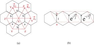
Figure 1: (Color online). (a) Bosons at filling factor $f$ are hopping on a triangular lattice ( red line ) which has three sublattices $X,Y,Z$. Its dual lattice is a honeycomb lattice ( black line ) which has two sublattices $a$ and $b$. (b) The bond phase factors in a dual honeycomb lattice at $f=1/3$ flux quanta per hexagon. The direction of the gauge field is important. At $f=2/3$, the bond phase factors are just complex conjugate of those at $f=1/3$.

The EBHM in both bi-partisan and frustrated lattices with various kinds of interactions and filling factors (commensurate or in-commensurate) is described by the following Hamiltonian pq1 ; gan ; five :

$$H = -t\sum_{\langle ij\rangle}(b^{\dagger}_{i}b_{j}+h.c.)-\mu\sum_{i}n_{i}+\frac{U}{2}\sum_{i}n_{i}(n_{i}-1)$$ (1)

$$+ V_{1}\sum_{\langle ij\rangle}n_{i}n_{j}+V_{2}\sum_{\langle\langle ik\rangle\rangle}n_{i}n_{k}+\cdots$$

where $n_{i}=b^{\dagger}_{i}b_{i}$ is the boson density, $t$ is the hopping amplitude, $U,V_{1},V_{2}$ are onsite, nearest neighbor and next nearest neighbor interactions between the bosons. The $\cdots$ may include further neighbor interactions, the dipole-dipole interaction dipolarss ; dipolarsstri , 3-body interaction 3body and possible ring-exchange interactions ring . The EBHM Eqn.1 can be realized by ultra-cold atoms loaded in optical lattices manybody . For example, using three coplanar beams of equal intensity having the three vectors making a $120^{\circ}$ angle with each other, the potential wells have their minima in a triangular lattice trilattice . The long range interactions $V_{1},V_{2},\cdots$ and the dipole-dipole interaction can be realized with dipolar bosons loaded in optical lattices junpolar . In this paper, we will use the DVM developed in pq1 ; univ to study various kinds of insulating phases and phase transitions in a triangular lattice (Fig.1a) at $1/3(2/3)$ fillings. With the gauge chosen in Fig.1b, the general effective vortex action in terms of the three modes $\xi_{l},l=0,1,2$ ( See Eqn.4 below ) invariant under all the PSG transformations upto sixth order terms was written down in tri . In the permutative representation basis $\phi_{l},l=0,1,2$ given by $\phi_{0}=\frac{1}{\sqrt{3}}(\xi_{0}+e^{-i\frac{2\pi}{3}}\xi_{1}+\xi_{2}),\phi_{1}=\frac{1}{\sqrt{3}}(e^{-i\frac{2\pi}{3}}\xi_{0}+\xi_{1}+\xi_{2}),\phi_{2}=\frac{1}{\sqrt{3}}(\xi_{0}+\xi_{1}+e^{-i\frac{2\pi}{3}}\xi_{2})$, the effective vortex action ${\cal L}_{SF}={\cal L}_{0}+{\cal L}_{1}+{\cal L}_{2}$ can be simplified to:

$${\cal L}_{0} = \sum_{l}|(\partial_{\mu}-iA_{\mu})\phi_{l}|^{2}+r|\phi_{l}|^{2}+(\epsilon_{\mu\nu\lambda}\partial_{\nu}A_{\lambda})^{2}/4$$

$${\cal L}_{1} = u(|\phi_{0}|^{2}+|\phi_{1}|^{2}+|\phi_{2}|^{2})^{2}-v[(|\phi_{0}|^{2}-|\phi_{1}|^{2})^{2}$$

$$+ (|\phi_{1}|^{2}-|\phi_{2}|^{2})^{2}+(|\phi_{2}|^{2}-|\phi_{0}|^{2})^{2}]$$

$${\cal L}_{2} = w[(\phi^{*}_{0}\phi_{1})^{3}+(\phi^{*}_{1}\phi_{2})^{3}+(\phi^{*}_{2}\phi_{0})^{3}+h.c.]$$ (2)

where $A_{\mu}$ is a non-compact $U(1)$ gauge field. When $r>0$, the bosons are in the superfluid state, $\langle\phi_{l}\rangle=0$ for every $l=0,1,2$. When $r<0$, the bosons are in a insulating state, $\langle\phi_{l}\rangle\neq 0$ for at least one $l$.

In order to develop a systematic way to use the vortex degree of freedoms in the honeycomb lattice to describe the symmetry breaking patters of the bosons in the triangular lattice, one has to derive the relation dof (namely Eqn.4 below) between the total vortex fields in the honeycomb lattice and the order parameters $\phi_{l}$ in Eqn.2. Then one need to first study five the energy spectrum of the vortices hopping in the honeycomb lattice in the presence of $f=p/q$ flux quantum per hexagon shown in Fig.1a. For the gauge chosen in Fig.1b, the vortex hopping Hamiltonian is $H_{v}=-t_{v}\sum_{\vec{x}}[|\vec{x}+\vec{\delta}\rangle e^{i2\pi fa_{1}}\langle\vec{x}|+|\vec{x}+\vec{\delta}\rangle\langle\vec{x}+\vec{a}_{2}|+|\vec{x}+\vec{\delta}\rangle\langle\vec{x}+\vec{a}_{1}+\vec{a}_{2}|+h.c.]$ where $\vec{x}=a_{1}\vec{a}_{1}+a_{2}\vec{a}_{2}$ and $\vec{x}+\vec{\delta},\vec{\delta}=1/3\vec{a}_{1}+2/3\vec{a}_{2}$ belong to the sublattice $a$ and $b$ respectively in Fig.1b. Following the Sec.3 of Ref.five , one can derive the Harper’s equation corresponding to $H_{v}$:

$$c^{a}_{m-1}(k_{x},k_{y}) + e^{ik_{y}}(1+e^{i(k_{x}+2\pi fm)})c^{a}_{m}(k_{x},k_{y})$$

$$= \epsilon(k_{x},k_{y})c^{b}_{m}(k_{x},k_{y}),$$

$$c^{b}_{m+1}(k_{x},k_{y}) + e^{-ik_{y}}(1+e^{-i(k_{x}+2\pi fm)})c^{b}_{m}(k_{x},k_{y})$$ (3)

$$= \epsilon(k_{x},k_{y})c^{a}_{m}(k_{x},k_{y})$$

where $m=0,1,\cdots,q-1$ and $a,b$ are two sublattices of the honeycomb lattice, the $-\pi/q\leq k_{x}\leq\pi/q,-\pi\leq k_{y}\leq\pi$ are inside the reduced Brillouin zone. At $q=3$, we are able to find the analytic expressions of the eigenvalues and the corresponding eigenvectors of the $6\times 6$ matrix in Eqn.3 at the 3 minima $(k_{x},k_{y})=(0,2\pi l/3),l=0,1,2$. The lowest eigenvalue is $\epsilon=-(1+2\cos 2\pi/9)t_{v}$, the corresponding eigenvector at $l=0$ is $(c^{a}_{m}(l=0),c^{b}_{m}(l=0))=[2\cos 4\pi/9+2\cos 2\pi/9+1,e^{-i\pi/3},2\cos 2\pi/9,2\cos 4\pi/9+2\cos 2\pi/9+1,2\cos 2\pi/9,e^{-i\pi/3}],~{}~{}m=0,1,2$. The eigenvectors at $l=1,2$ can be achieved by the magnetic translation pq1 ; tri along $\vec{a}_{1}$: $c^{a}_{m}(l)=c^{a}_{m}(l=0)\omega^{-ml},c^{b}_{m}(l)=c^{b}_{m}(l=0)\omega^{-ml}\omega^{l}$ where $\omega=e^{i2\pi f}$. The eigenfunctions at the three minima $(k_{x},k_{y})=(0,2\pi l/3)$ are $\psi^{a}_{l}(\vec{x})=\sum^{q-1}_{m=0}c^{a}_{m}(l)e^{i2\pi f(ma_{1}+la_{2})},\psi^{b}_{l}(\vec{x})=\sum^{q-1}_{m=0}c^{b}_{m}(l)e^{i2\pi f(ma_{1}+la_{2})}$. Then one can write the total vortex fields at the sublattice a and b in the Fig.1 as the expansion in terms of the three eigenfunctions:

$$(\Phi^{a}(\vec{x}),\Phi^{b}(\vec{x}))^{T}=\sum^{2}_{l=0}(\psi^{a}_{l}(\vec{x}),\psi^{b}_{l}(\vec{x}))^{T}\xi_{l}$$ (4)

where the $T$ means the transpose and the three coefficients $\xi_{l},l=0,1,2$ are the three vortex order parameters. The effective action Eqn.2 was written in the permutative representation $\phi_{l}$.

Plugging the mean field solutions of all insulating states where $r<0$ in Eqn.2 into Eqn.4, one can construct the following gauge invariant quantities hightc : the densities at different sites in sublattices $a$ and $b$:

$$|\Phi_{a}(\vec{x})|^{2},~{}~{}~{}~{}~{}|\Phi_{b}(\vec{x})|^{2}$$ (5)

and the bond quantities between sublattice $a$ and sublattice $b$ :

$$\Phi^{\dagger}_{b}(\vec{x})e^{i2\pi fa_{1}}\Phi_{a}(\vec{x})=K-iI$$ (6)

where $\vec{x}$ belongs to the same unit cell shown in Fig.1b. All the other bonds having no phase factor from the gauge field. The real part $K$ gives the kinetic energy between the two sites. The imaginary part $I$ gives the current between the two sites. By using the Eqn.5, especially Eqn.6, one can extract the corresponding symmetry breaking patterns of bosons in the direct triangular lattice. In the following, we discuss the 3 possible insulating states of Eqn.2 where $r<0$ respectively.

(1) If $v>0$, the system is in the Ising limit, only one of the 3 vortex fields condense. For example, substituting $\phi_{0}=1,\phi_{1}=\phi_{2}=0$ into Eqns.4-6, one can evaluate the vortex densities, kinetic energy and the current in the dual honeycomb lattice. For simplicity, we only show the currents in Fig.2a which are obviously conserved. It is important to observe that the chirality $\chi_{p}=\sum_{p}I$ around any hexagon $p$ leads to the boson density at the center of the hexagon $n_{p}=1/3+\chi_{p}$. Then we can calculate the densities at the three sublattices: $n_{x}=1/3+6\delta I>1/3,n_{y}=n_{z}=1/3-3\delta I<1/3$ with the constraint $n_{x}+n_{y}+n_{z}=1$ where the $I$ is the current flowing around the $X$ lattice site in Fig.2a. The $\delta\sim n_{x}-n_{y}>0$ can be taken as the CDW order parameter measuring the distance from the SF to the CDW transition.

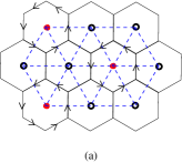
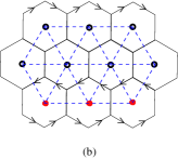
Figure 2: (Color online). (a) The X-CDW state in the Ising limit $v>0$ at $f=1/3$. (b) The period 3 stripe phase in the easy plane limit $v<0,w<0$ at $f=1/3$. At $f=2/3$, one can just reverse the current flow and perform a particle and hole transformation on $f=1/3$, namely, exchange particles ( red dots ) and vacancies ( black empty circles ).

(2) If $v<0$, the system is in the easy-plane limit, all the three vortex fields have equal magnitude $\phi_{l}=|\phi|e^{i\theta_{l}}$ and condense. There are also two distinguished cases:

(2a) If $v<0,w<0$, the mean field solution tri is $\theta_{1}-\theta_{0}=2\pi m/3,\theta_{2}-\theta_{0}=2\pi n/3$ where $m,n=0,1,2$. Substituting $\theta_{0}=\theta_{1}=\theta_{2}=0$ into Eqns.4-6, one can evaluate the vortex densities, kinetic energy and the current in the dual honeycomb lattice. For simplicity, we only show the currents in Fig.2b. Similar arguments as in (1) shows that this is a stripe phase.

(2b) If $v>0,w>0$, one of the 18 equivalent solutions tri is $\theta_{1}-\theta_{0}=\theta_{0}-\theta_{2}=2\pi/9$, then $\theta_{1}-\theta_{2}=4\pi/9$. Substituting this solution into Eqns.4-6, one can evaluate the vortex densities, kinetic energy and the currents shown in Fig.3. It is important to realize there are two independent currents $I_{1}$ and $I_{2}$ flowing in Fig.3. Similar to (1), we can calculate the three different densities: $n_{r}=1/3+2\delta[I_{1}+(I_{1}-I_{2})]>1/3,n_{g}=1/3+2\delta[I_{2}+(I_{2}-I_{1})]>1/3,n_{b}=1/3-2\delta[I_{1}+I_{2}]<1/3$ with the constraint $n_{r}+n_{g}+n_{b}=1$ where $I_{1}=\sin\frac{3\pi}{9}+\sin\frac{2\pi}{9}>I_{2}=\sin\frac{2\pi}{9}+\sin\frac{\pi}{9}$. The $\delta$ can be taken as the CDW-VBS order parameter measuring the distance from the SF to the CDW+VBS transition. When one tunes the density $n_{b}=0$, then $n_{r}=\frac{I_{1}}{I_{1}+I_{2}}>n_{g}=\frac{I_{2}}{I_{1}+I_{2}}$ with $n_{r}/n_{g}=I_{1}/I_{2},n_{r}+n_{g}=1$.

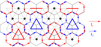
Figure 3: (Color online). The CDW-VBS phase in a triangular lattice at $f=1/3$ in the easy plane limit $v<0,w>0$. Shown is $\theta_{0}=0,\theta_{1}=2\pi/9,\theta_{2}=-2\pi/9$ case. There are two different vortex currents flowing in the dual honeycomb lattice. The red current is $I_{1}=\sin\frac{3\pi}{9}+\sin\frac{2\pi}{9}$, the green current $I_{2}=\sin\frac{\pi}{9}+\sin\frac{2\pi}{9}$. The vortex currents are conserved at all the lattice points. The two different vortex currents in a dual honeycomb lattice imply 3 different densities $n_{r},n_{g},n_{b}$ in a triangular lattice listed in the text. At $f=2/3$, one can just reverse the current flow and perform a particle and hole transformation on $f=1/3$.

It is important to observe that the vortex fields vanish at the centers of both the red loop and the green loop, therefore, both the kinetic energy and the current emanating from the centers vanish. This fact indicates that there are local SF (or VBS order) around the these two dual lattice points as shown by the red and green triangles in Fig.3. It is interesting to compare this fact with the known result that the interacting bosons in a Kagome lattice at $f=1/2$ five ; ka1 are always in a SF state due to the localization of the vortices (a flat vortex band). The crucial difference is that here there is only a local SF around the the centers of the red loop and the green loop, while there is a global SF across the whole lattice in the latter. We need also stress that the vortex field is non-vanishing at the black point, so only the current vanishes, but the kinetic energy does not vanish, it shows that there are local CDW around the dual lattice point as shown by black circles in Fig.3. So this state has both VBS and CDW order which is a hybrid state unique to a frustrated lattice.

Now we will determine quantitatively the CDW and VBS ordering patterns of the CDW-VBS phase in Fig.3. The CDW component of the CDW+VBS phase is given by:

$$\rho_{CV}(\vec{x}) = 1/3+4\delta\sqrt{\frac{I^{2}_{1}-I_{1}I_{2}+I^{2}_{2}}{3}}[-\cos(\frac{2\pi}{3}x+\frac{5\pi}{18})$$ (7)

$$+ \cos(\frac{2\pi}{3}y+\frac{\pi}{18})+\cos(\frac{2\pi}{3}(x-y)+\frac{\pi}{18})]$$

where $\delta$ is the CDW order parameter and $I_{1},I_{2}$ are the vortex currents in Fig.3. The VBS component of the CDW+VBS phase is given by:

$$B_{1}(\vec{x}) = B_{d}(\vec{x})=c\delta(I_{1}+I_{2})(1+2\cos\frac{2\pi}{3}(x+y))$$

$$+ 2c\delta\sqrt{I^{2}_{1}-I_{1}I_{2}+I^{2}_{2}}[\cos(\frac{2\pi}{3}x+\frac{2\pi}{9})$$

$$+ \cos(\frac{2\pi}{3}y-\frac{2\pi}{9})+\cos(\frac{2\pi}{3}(x-y)-\frac{2\pi}{9})]$$

$$B_{2}(\vec{x}) = B_{1}(\vec{x}-\vec{a}_{1})$$ (8)

where the $c$ is an overall constant which can not be determined from the PSG symmetry based on the DVM. When comparing with the CDW order in Eqn.7, we can see that in addition to the 3 ordering wave vectors $\vec{Q}_{\alpha}=2\pi/3(1,0),2\pi/3(0,1),2\pi/3(1,-1),\alpha=1,2,3$, there is also a new VBS ordering wave vector $\vec{Q}_{VBS}=2\pi/3(1,1)$. It is this new ordering wave vector which makes the determination of the VBS order inside the CDW-VBS phase possible by the QMC trinnn and its detection possible by light scattering experiments of cold atoms loaded on optical lattices bragg .

By extending the DOF in pq1 for a square lattice to the triangular lattice, the authors in Ref.tri identified a bubble CDW phase in the $v>0,w>0$ case. This bubble CDW phase has only one vortex current $I$ flowing in the dual honeycomb lattice, so there is just two different densities. Furthermore, there is no VBS order. Therefore the bubble phase is completely different from the CDW-VBS phase in Fig.3. This discrepancy indicates the DOF developed in pq1 ; tri may have intrinsic difficulties. Some general problems associated with the DOF are examined in long .

The EBHM of the hard core bosons with $U=\infty,V_{1}>0,V_{2}>0$ was studied by QMC in trinnn . A period-3 stripe solid state in Fig.2b is found at $f=1/3$. The dual vortex effective action to describe the transition from the SF to the stripe solid is given by Eqn.2 in the easy plane limit $r<0,v<0,w<0$. Unfortunately, the very interesting CDW-VBS phase in Fig.3 was not searched in the QMC in trinnn in any parameter regimes. In order to identify this phase, in addition to the QMC calculations of the SF density and the density structure factor in trinnn , a bond structure factor shown in Eqn.8 need also be studied to identify the VBS ordering where there is an additional new VBS ordering wavevector $\vec{Q}_{VBS}=\frac{2\pi}{3}(1,1)$. The authors in 3body studied the EBHM Eqn.1 with a three-body interaction in a 1 dimensional lattice by QMC. They also found a solid state with the coexistence of CDW and VBS at $f=2/3$. It would be very interesting so do a QMC on a triangular lattice with the 3-body interaction to see if the 3-body interaction can stabilize the CDW-VBS phase in Fig.3.

When our method is applied to bipartite lattices long , it can recover all the previously known phases in pq1 ; univ . When it is applied to a Kagome lattice long , we also find another CDW+VBS states in the easy plane limit $v<0,w>0$, so we believe that the CDW-VBS state may be a common and robust state in any frustrated lattices. It is interesting to identify such kind of states by QMC simulations and realize them in near future cold atom experiments. The dual relations between the correlations of bosons and those of vortices explored in this paper should also shed lights on exploring duality relations between correlations functions in other strongly correlated physical systems.

We thank Fuchun Zhang and Zidan Wang for the hospitality during our visit at Hong Kong university which initiated the collaboration. YC was supported by the NSFC-10874032 and 11074043, the State Key Programs of China (Grant no. 2009CB929204) and Shanghai Municipal Government. JY was supported by NSF-DMR-1161497, NSFC-11074173,11174210, Beijing Municipal Commission of Education under grant No.PHR201107121, at KITP was supported in part by the NSF under grant No. PHY-0551164. JY thanks Han Pu for his hospitality during his visit at Rice university where part of this work was done.

References

- (1) For a review on duality in field theory, see R. Savit, Rev. Mod. Phys. 52, 453 (1980).
- (2) C. Dasgupta and B. I. Halperin , Phys. Rev. Lett. 47, 1556 (1981); M. E. Peskin, Ann. Phys. N.Y. 113, 122 (1978).
- (3) C. P. Herzog, P. Kovtun, S. Sachdev, and D.T. Son, Phys. Rev. D 75, 085020 (2007).
- (4) L. Balents, L. Bartosch, A. Burkov, S. Sachdev, and K. Sengupta, Phy. Rev. B 71, 144508 (2005).
- (5) A.A. Burkov and L. Balents, Phys. Rev. B 72, 134502 (2005).
- (6) L. Jiang and J. Ye, J. Phys. Cond. Matt. 18, 6907 (2006).
- (7) J. Ye, Nucl. Phys. B 805, 418 (2008).
- (8) G. Murthy, D. Arovas, and A. Auerbach, Phys. Rev. B 55, 3104 (1997).
- (9) B. Capogrosso-Sansone, et al, Phys. Rev. Lett. 104, 125301 (2010).
- (10) L. Pollet, J. D. Picon, H. P. B chler, and M. Troyer, Phys. Rev. Lett. 104, 125302 (2010).
- (11) J. R. Armstrong, N. T. Zinner, D. V. Fedorov and A. S. Jensen, Euro. Phys. Lett. 91 16001 (2010).
- (12) B. Capogrosso-Sansone, et al, Phys. Rev. B 79, 020503(R) (2009).
- (13) H. P. B chler, et.al, Phys. Rev. Lett. 95, 040402 (2005).
- (14) For a review, see I. Bloch, J. Dalibard, and W. Zwerger, Rev. Mod. Phys. 80, 885 (2008).
- (15) G. Grynberg, B. Lounis, P. Verkerk, J.Y. Courtois, and C. Salomon, Phys. Rev. Lett. 70, 2249 (1993).
- (16) K.-K. Ni, et al, Science 322, 231 (2008).
- (17) J. Ye, J.M. Zhang, W.M. Liu, K.Y. Zhang, Yan Li, W.P. Zhang, Phys. Rev. A 83, 051604 (R) (2011).
- (18) Such a relation is not needed in the DOF which was constructed from general symmetry principles in pq1 ; tri .
- (19) For the importations of the gauge invariant electron Green functions in the pseudo-gap regime of the high temperature superconductors and its connections to the angle-resolved photo-emission spectroscopy (ARPES), see J. Ye, Phys. Rev. Lett. 87, 227003 (2001); Phys. Rev. B. 65, 214505 (2002); Phys. Rev. B. 67, 115104 (2003).
- (20) K. Sengupta, S. V. Isakov, and Y. B. Kim, Phys. Rev. B 73, 245103 (2006).
- (21) R.G. Melko, A. Del Maestro, and A.A. Burkov, Phys. Rev. B 74, 214517 (2006).
- (22) Jinwu Ye and Yan Chen, unpublished.