Dynamics of matter-wave solitons in a time-modulated two-dimensional optical lattice.

Abstract

By means of the variational approximation (VA) and systematic simulations, we study dynamics and stability boundaries for solitons in a two-dimensional (2D) self-attracting Bose-Einstein condensate (BEC), trapped in an optical lattice (OL) whose amplitude is subjected to the periodic time modulation (the modulation frequency, $\omega$, may be in the range of several KHz). Regions of stability of the solitons against the collapse and decay are identified in the space of the model’s parameters. A noteworthy result is that the stability limit may reach the largest ($100\%$) modulation depth, and the collapse threshold may exceed its classical value in the static lattice (which corresponds to the norm of Townes soliton). Minimum norm $N_{\min}$ necessary for the stability of the solitons is identified too. It features a strong dependence on $\omega$ at a low frequencies, due to a resonant decay of the soliton. Predictions of the VA are reasonably close to results of the simulations. In particular, the VA helps to understand salient resonant features in the shape of the stability boundaries observed with the variation of $\omega$.

I Introduction

A challenging subject in the study of dynamical patterns in Bose-Einstein condensates (BECs) is the investigation of matter-wave solitons in multidimensional settings. Various routes leading to the creation of stable 2D and 3D solitons have been elaborated theoretically. The proposed approaches have much in common with their counterparts developed for the stabilization of 2D and 3D spatiotemporal solitons in nonlinear optics, see review Review . However, thus far, only effectively one-dimensional (1D) matter-wave solitons have been created in experiments which used cigar-shaped traps to confine the condensate experiment (the actual shape of the soliton may be nearly three-dimensional, but it is intrinsically self-trapped only in the longitudinal direction). A phenomenon which impedes the stabilization of truly multidimensional solitons is the occurrence of collapse in 2D and 3D condensates with attraction between atoms. As demonstrated in Refs. BBB ; BBB2 ; BBB3 , a universal method for the stabilization of matter-wave solitons in the multidimensional setting may be provided by optical lattices (OLs), i.e., periodic potentials which are induced, through interference patterns, by coherent laser beams illuminating the condensate in opposite directions (in principle, similar methods may be applied to a gas of polaritons, where an evidence of the BEC state was recently reported too Kasprzak:2006a ). The stabilization of 2D and 3D solitons is possible with the help of the fully-dimensional OL, whose dimension is equal to that of the entire space, and by low-dimensional lattices, whose dimension is smaller by one. The latter means quasi-1D and quasi-2D OLs in the 2D and 3D space, respectively BBB2 ; Barcelona . OLs may also support solitons of a completely different type, namely, gap solitons in BEC (of any dimension) with repulsion between atoms. In this case, the solitons emerge due to the interplay between the repulsive nonlinearity and the negative effective mass in parts of the linear bandgap spectrum generated by the OL gap1D . Although gap solitons cannot represent the ground state of the respective system, they are dynamically stable objects GSstability . The creation of effectively 1D gap solitons, composed of $\simeq 250$ atoms of ⁸⁷Rb, was reported in Ref. Eiermann:2004a , see also review OliverMorsch:2006a . Multidimensional (chiefly, 2D) gap solitons gap2D , and “semi-gap” solitons (which look like gap solitons in one direction, and regular solitons in the other semi-gap ) were predicted too gap2D , but not yet observed in the experiment. Stable gap solitons, in 1D and 2D settings alike, can be supported not only by periodic OLs, but also by quasi-periodic ones HidetsuguSakaguchi:2006a .

It is relevant to note that the presence of the lattice, defining a particular spatial scale in the system (the OL period), introduces an effective nonlocality. On the other hand, a nonlocality can be directly induced by long-range interactions between atoms carrying dipolar moments. In this way, it has been demonstrated that the interplay between the local repulsion and long-range attraction may also support stable 2D solitons, both isotropic DDiso and anisotropic DDaniso ones.

Another theoretically elaborated stabilization technique relies on periodic time modulation of the effective nonlinearity coefficient, which may be provided by the Feshbach-resonance effect in a low-frequency ac magnetic field applied to the condensate. It has been demonstrated that this method can stabilize 2D fundamental solitons, but not 3D ones FRM (the stabilization of 3D solitons and their bound complexes is possible under a combined action of this technique and a quasi-1D OL Warsaw ; the application of the Feshbach-resonance technique to matter waves trapped in usual OLs Mason , as well as in parabolic traps Fatkhulla , was studied too). This approach to the creation of stable 2D matter-wave solitons followed the earlier elaborated mechanism providing for the stabilization of (2+1)-dimensional optical spatial solitons in the model of a bulk medium built as a periodic concatenation of layers with self-focusing and self-defocusing Kerr nonlinearity Isaac . It should be noted, however, that very accurate simulations of the so stabilized 2D solitons in the framework of the respective Gross-Pitaevskii equation (GPE) demonstrate that they may be subject to an extremely slow decay Itin .

The methods using the periodic modulation of the nonlinearity belong to a broad class of techniques relying on the periodic management of solitons book . In terms of the BEC in one dimension, another relevant example representing this class is the lattice management in the model where the strength of the OL is subjected to periodic time modulation Dalfovo ; Thawatchai (in the experiment, this was used as a method to excite the condensate experiment-OL ). The main result of the analysis of the model including the lattice management in combination with the self-repulsive nonlinearity, reported in Ref. Thawatchai , was identification of stability limits for several families of gap solitons in this setting (fundamental solitons, double-hump bound states, etc.). Also belonging to this general class are settings based on the periodic modulation in time of the strength of a parabolic potential trap which confines the condensate trap-modulation , and periodic modulation of the transverse trapping frequency which supports cigar-shaped BEC configurations. In the latter case, the “management” may induce Faraday waves in the condensate, as was predicted theoretically Faraday-theory and demonstrated experimentally Engels . It is also relevant to mention that another variety of the ”management” was proposed very recently, with the aim to stabilize 2D matter-wave solitons: driven Rabi oscillations in a mixture of two mutually interconvertible BEC species (different states of the same atom), with self-attractive and self-repulsive intra-species interactions Randy .

II The model and outline of the paper

A natural extension of the studies outlined above is the application of the lattice-management technique to multidimensional solitons. This topic includes several distinct problems, depending on the sign of the intrinsic nonlinearity. In the 1D setting, the lattice management for solitons in the attraction model is not a fundamentally important issue, because stable 1D solitons in the self-attractive condensate exist without any lattice experiment . However, the model with the intrinsic attraction poses a new problem in the 2D case, as, in the absence of the lattice, 2D solitons are unstable against the collapse, and, as said above, the simplest way to suppress the instability is provided by the use of the quasi-1D OL BBB2 . Therefore, it may be interesting to identify stability limits for 2D solitons in the attractive model with the quasi-1D lattice whose strength is subjected to the periodic time modulation; in particular, one may be wondering if the solitons may survive in the case when the modulation depth attains its maximum, so that the lattice periodically vanishes. This problem was a subject of recent work Thawatchai2 , which was also dealing with collisions between the 2D solitons, that may move freely in the unconfined direction. It was found that the actual stability region is quite limited: typically, the solitons loose their stability before the modulation depth attains $50\%$.

The objective of the present work is to construct soliton families and identify their stability boundaries in the 2D attractive model with the full 2D lattice subject to the time-periodic modulation. In the normalized form, the respective two-dimensional GPE for mean-field wave function $\Psi\left(x,y,t\right)$ is

$$i\frac{\partial\Psi}{\partial t}=-\frac{1}{2}\left(\frac{\partial^{2}}{\partial x^{2}}+\frac{\partial^{2}}{\partial y^{2}}\right)\Psi-\left|\Psi\right|^{2}\Psi-V_{0}\left[1+\frac{\varepsilon}{2}\cos(\omega t)\right]\left[\cos\left(2x\right)+\cos\left(2y\right)\right]\Psi,$$ (1)

where $t$ is time, $\left(x,y\right)$ are coordinates in the 2D plane (scaled so as to fix the OL period equal to $\pi$), and $V_{0}$ is the strength of the lattice, while $\varepsilon$ and $\omega$ are the amplitude and frequency of its temporal modulation. Coefficient $-1$ in front of the nonlinear term in Eq. (1) implies that the nonlinearity is attractive. In the case of the quasi-1D lattice BBB2 ; Thawatchai2 , term $\cos(2y)$ is dropped from the potential in Eq. (1). Actually, $V_{0}$ is measured in units of the recoil energy of atoms trapped in the OL. For a typical case of atoms of ⁷Li loaded in the OL with the period on the order of $\mu$m, a characteristic value of the scaled frequency, $\omega\sim 2$ (see below), corresponds, in physical units, to the modulation rate on the order of several KHz.

An experimental implementation of the model may be provided by periodic attenuation of the intensity of the laser beams that create the OL. Since this management mode cannot change the sign of the OL’s amplitude, the modulation coefficient in Eq. (1) is restricted to interval $0\leq\varepsilon\leq 2$. We, chiefly, follow this restriction below. On the other hand, Eq. (1) with the modulated potential that formally corresponds to $\varepsilon\rightarrow\infty$, viz., $-V_{0}\cos(\omega t)\left[\cos\left(2x\right)+\cos\left(2y\right)\right]$, may be realized as a superposition of several moving OLs Staliunas:2007a (a 1D counterpart of that setting was introduced in Ref. Staliunas:2006a ). In works Staliunas:2006a and Staliunas:2007a it was demonstrated that such potentials, if combined with the self-repulsive nonlinearity, give rise to anomalously narrow subdiffractive gap solitons, for which the usual second-order operator of the kinetic energy is, effectively, replaced by a fourth-order operator. On the other hand, a piecewise-constant time-periodic modulation mode was considered, for both periodic and quasi-periodic 2D potentials, in recent work Gena (also in the combination with the self-repulsive nonlinearity). The result was generation of a multi-soliton lattice, starting from an initial localized state.

The rest of the paper is organized as follows. In Section III, we elaborate the variational approximation (VA) for the analysis of the dynamics of fundamental 2D solitons in the model based on Eq. (1). In Section IV, results of systematic direct simulations of the soliton evolution in Eq. (1) are reported, and compared with predictions of the VA. The results are summarized in the form of stability regions for the solitons in the model with the time-modulated OL. The most noteworthy finding reported in Section IV is that, depending on $\omega$, the solitons may remain stable up to the maximum ($100\%$) modulation depth, in contrast to the shallow modulation that limited the stability of the solitons supported by the quasi-1D OL Thawatchai2 . It is also worthy to mention a multi-resonance shape featured by the stability boundary in the $\left(\omega,\varepsilon\right)$ plane, and an increase of the collapse threshold (defined in terms of the soliton’s norm) provided by the time-modulated OL, in comparison with the static lattice, i.e., the threshold may exceed the norm of the Townes soliton. The minimum norm necessary for the stability of the solitons, $N_{\min}$, is identified too, as a function of $\omega$ and $\varepsilon$ (this characteristic was considered earlier only in the static model Salerno ). Due to the possibility of a resonantly enhanced decay of the soliton, $N_{\min}$ features a strong dependence on $\omega$ at low frequencies. The paper is concluded by Section V.

III The variational approximation

III.1 Effective Lagrangian

Variational methods have been quite useful in many problems of nonlinear optics and BEC Desaix ; VA ; BBB ; BBB2 ; FRM ; book . To apply the VA to the present model, we notice that Eq. (1) can be derived from Lagrangian $L=\int_{-\infty}^{+\infty}\mathcal{L}dx$, with density

$$\mathcal{L} =\frac{i}{2}\left(\Psi^{\ast}\Psi_{t}-\Psi\Psi_{t}^{\ast}\right)-\frac{1}{2}\left(\left|\Psi_{x}\right|^{2}+\left|\Psi_{y}\right|^{2}\right)+\frac{1}{2}\left|\Psi\right|^{4}$$

$$+V_{0}\left[1+\frac{\varepsilon}{2}\cos(\omega t)\right]\left[\cos\left(2x\right)+\cos\left(2y\right)\right]\left|\Psi\right|^{2},$$ (2)

where the asterisk stands for the complex conjugation. Following Refs. BBB and BBB2 , we adopt the isotropic ansatz for the soliton,

$$\Psi_{\mathrm{ans}}\left(x,y,t\right)=A(t)\exp\left(i\phi(t)+\frac{i}{2}b(t)r^{2}-\frac{r^{2}}{2W^{2}(t)}\right),$$ (3)

where $r^{2}\equiv x^{2}+y^{2}$, and all variables $A(t),$ $\phi(t),$ $b(t),$ and $W(t)$ (amplitude, phase, radial chirp, and radial width, respectively) are real. Tractable, although rather cumbersome, variational equations may also be generated by an anisotropic generalization of ansatz (3), with different widths and chirps along axis $x$ and $y$. However, subsequent analysis of those equations does not predict stable anisotropic solitons.

The substitution of the ansatz in Eq. (2) and calculation of the integrals yield the effective Lagrangian,

$$L_{\mathrm{eff}} =-N\frac{d\phi}{dt}-\frac{N}{2W^{2}}+\frac{N^{2}}{4\pi W^{2}}+2V_{0}\left[1+\frac{\varepsilon}{2}\cos(\omega t)\right]Ne^{-W^{2}}$$

$$-\frac{1}{2}\frac{db}{dt}NW^{2}-\frac{1}{2}b^{2}NW^{2},$$ (4)

where $N\equiv\pi A^{2}W^{2}$. The first Euler-Lagrange equation following from effective Lagrangian (4), $\delta\left(\int L_{\mathrm{eff}}dt\right)/\delta\phi=0$ ($\delta/\delta\phi$ stands for the variational derivative of the action functional), is tantamount to the conservation of the norm of the wave function, which is the single dynamical invariant of Eq. (1). Indeed, the norm of ansatz (3) is

$$\int\int\left|\Psi_{\mathrm{ans}}(x,y)\right|^{2}dxdy=\pi A^{2}W^{2}\equiv N.$$ (5)

The second Euler-Lagrange equation, $\delta\left(\int L_{\mathrm{eff}}dt\right)/\delta b=0$, reduces to the well-known expression for the chirp in terms of the time derivative of the width Desaix ; VA , $b=W^{-1}\left(dW/dt\right)$. Using this relation, the next variational equation, which accounts to $\partial L_{\mathrm{eff}}/\partial\left(W^{2}\right)=0$ [since Lagrangian (4) does not contain $dW/dt$] can be cast in the following final form,

$$\frac{d^{2}W}{dt^{2}}=\frac{1-N/\tilde{N}_{\max}}{W^{3}}-4V_{0}\left[1+\frac{\varepsilon}{2}\cos(\omega t)\right]W\exp\left(-W^{2}\right),$$ (6)

where $\tilde{N}_{\max}\equiv 2\pi$ is the well-known VA prediction Desaix for the critical (maximum) norm in the 2D space, which separates collapsing solutions at $N>\tilde{N}_{\max}$, i.e., ones with $W(t)\rightarrow 0,~{}A(t)\rightarrow\infty$ at $t\rightarrow t_{\mathrm{collapse}}$ [for $V_{0}=0$ and initial conditions $W(t=0)=W_{0}$ and $dW/dt(t=0)=0$, the collapse time predicted by Eq. (6) is $t_{\mathrm{collapse}}=W_{0}^{2}\left(N/\tilde{N}_{\max}-1\right)^{-1/2}$], and noncollapsing ones at $N<\tilde{N}_{\max}$.

III.2 Analysis of variational equation.

The actual maximum value of $N$, found numerically from Eq. (1) with $V_{0}=0$ (it gives the norm of the Townes soliton Berge ), is

$$N_{\max}=5.85\approx\allowbreak 0.93\tilde{N}_{\max},$$ (7)

which characterizes the accuracy of the VA. For the condensate of ⁷Li atoms, a typical collapse threshold corresponds to the number of atoms $\lesssim 10^{4}$.

Equation (6) helps one to understand what may happen to the 2D soliton under the action of the weak “management”, with $\varepsilon/2\ll 1$. First, for $\varepsilon=0$, Eq. (6) predicts a stable equilibrium position, which is given by a smaller root of equation

$$W_{0}^{4}\exp\left(-W_{0}^{2}\right)=\frac{1-N/\tilde{N}_{\max}}{4V_{0}}$$ (8)

(the larger root gives an unstable solution). Then, the linearization of Eq. (6) (still with $\varepsilon=0$) yields the eigenfrequency of small oscillations around $W=W_{0}$,

$$\omega_{0}=\frac{\sqrt{2\left(1-N/\tilde{N}_{\max}\right)\left(2-W_{0}^{2}\right)}}{W_{0}^{2}}.$$ (9)

For instance, in the example considered in the next section (see Fig. 5 below), with $1-N/\tilde{N}_{\max}=0.155$ and $V_{0}=0.25$, the relevant root of Eq. (8) is $W_{0}\approx 0.71$, and Eq. (9) yields $\omega_{0}\approx 1.35$. Keeping quadratic and cubic terms in the expansion of Eq. (6) in powers of $w(t)\equiv W(t)/W_{0}-1$ around $W$ leads to a standard equation of driven nonlinear oscillations. In particular, in the near-critical situation, i.e., for $1-N/\tilde{N}_{\max}\ll 1$, this equation takes the form of

$$\frac{d^{2}w}{dt^{2}}+16V_{0}w-24V_{0}w^{2}+40V_{0}w^{3}=-2\varepsilon V_{0}\cos(\omega t)-2\varepsilon V_{0}\cos\left(\omega t\right)w.$$ (10)

It predicts the lowest-order direct resonance when $\omega$ is close to $\omega_{0},$ the parametric resonance at $\omega$ close to $2\omega_{0}$, and higher-order resonances at $\omega=n\omega_{0}$, with $n=2,3,4,..$ Landau . The resonances may help to stabilize the 2D soliton against the collapse, as, increasing the amplitude of its intrinsic oscillations, the soliton spends less time in the “dangerous zone” with small width, that might be a starting point for the collapse. On the other hand, effectively stretching the soliton, the resonances may destabilize it against decay into radiation, at smaller values of $N$. Both trends are observed in numerical simulations, as shown below. Comparison of predictions following from a numerical solution of full variational equation (6) and direct simulations of Eq. (1) is presented in the next section.

IV Numerical results

IV.1 The simulation mode

Systematic simulations of Eq. (1) were performed by means of the split-step method Press , in the $\left(x,y\right)$ domain of size $256\times 256$ or $512\times 512$. The simulations were run with the Gaussian initial configuration,

$$\Psi(x,y,0)=A_{0}\exp\left(-q\left[\left(x-x_{0}\right)^{2}+\left(y-y_{0}\right)^{2}\right]\right),~{}q>0,$$ (11)

whose norm is $N=\pi A_{0}^{2}/q$ [cf. ansatz (3)]. Taking $N<N_{\max}$, as well as $N$ slightly exceeding $N_{\max}$ [recall $N_{\max}$, the critical value of the norm for the onset of the free-space collapse, is given by Eq. (7)], it was quite easy to find stable solitons which keep their shape despite the temporal modulations imposed by the “management”, see generic examples in Figs. 1 and 2. The former figure presents comparison of the initial and final shapes of the soliton, while the latter one displays the evolution of the soliton’s amplitude in the course of its self-adjustment to the stable shape.

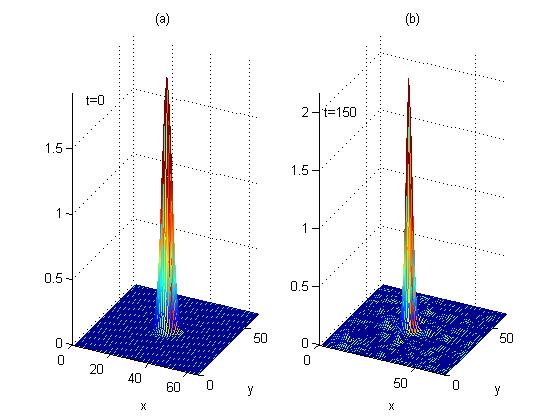
Figure 1: (Color online) A typical example of a stable 2D soliton, as obtained from the numerical solution of Eq.(1) with $V_{0}=0.65$, $\varepsilon=0.5$, $\omega=1.35$, and initial configuration (11) with $A_{0}=1.39$, $q=0.5$, whose norm, $N=6.07$, exceeds the collapse threshold in the static model, $N_{\max}\approx 5.85$. The panels display the density distribution, $\left|\Psi(x,y,t)\right|^{2}$, at $t=0$ (a) and $t=150$ (b).

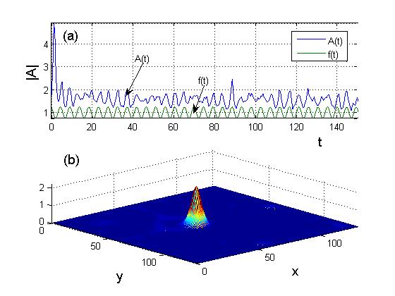
Figure 2: (Color online) (a) The evolution of the amplitude of the stable soliton, $|A|\equiv\left|\Psi\left(x=x_{0},y=y_{0}\right)\right|$, for the same parameters as in Fig. 1, except for $V_{0}=0.5$ ($|A|$ has the same meaning in other figures). Curve $f(t)$ shows the modulation function in Eq.(1), $1+\left(\varepsilon/2\right)\sin\left(\omega t\right)$; (b) The shape of the soliton at $t=150$.

The soliton shapes displayed in Figs. 1 and 2 are confined, essentially, to a single cell of the OL (similar to results reported in previous works BBB ; BBB3 ; Barcelona ). Roughly the same shapes would be observed in a parabolic trapping potential; however, the difference is that, if the nonlinearity is too weak, the OL cellular potential cannot suppress the tunnel decay of the localized pulses Salerno , therefore the decay is observed at smaller values of $N$, as shown below.

As said above, in the 2D equation with $V_{0}=0$ localized configurations with $N>N_{\max}=5.85$ suffer collapse, while those with $N<N_{\max}$ decay. The static OL stabilizes 2D solitons in the latter case, but it cannot arrest the collapse of initial localized states with $N>N_{\max}$ BBB ; BBB2 ; BBB3 . The numerical analysis of the model with the quasi-1D lattice potential subjected to the periodic time modulation did not reveal stable solitons with $N>N_{\max}$ either Thawatchai2 . As shown in Fig. 3, in the present model the periodic time modulation of the two-dimensional OL potential makes it possible to stabilize the solitons both at $N<N_{\max}$ and in some interval above $N_{\max}$. The actual increase of critical norm is not large, but the very fact that the constraint $N\leq N_{\max}$ can be broken is an interesting result, as it has never been reported before, to the best of our knowledge.

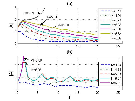
Figure 3: (Color online) The evolution of the soliton’s amplitude, as obtained from the numerical solution of Eq. (1) for $\varepsilon=0.5$ and $\omega=1$ and different values of norm $N$ of initial configuration (11) (higher curves correspond to larger $N$). (a) The model without the optical lattice, $V_{0}=0$. In this case, all configurations with $N<N_{\max}\approx 5.85$ decay, while the ones with $N>N_{\max}$ suffer the collapse. (b) In the presence of the time-modulated optical lattice with $V_{0}=0.5$, the 2D solitons may be stable, including some values of $N$ above $N_{\max}$. In particular, the soliton is stable at $N=6.01\approx 1.03N_{\max}$, while it collapses for $N=6.09$, at $t=1.49$. If $N$ is too small, $N<N_{\min}$, the soliton gradually decays into radiation, see Fig. 7 below. In panel (b), the curve for $N=3.14$, which is slightly smaller than the corresponding value of $N_{\min}$, also shows the slow decay of the soliton.

IV.2 Comparison with the variational approximation

Comparison of the predictions of the VA with numerical results in two typical cases (for stable and decaying solitons, corresponding to $N=5.4$ and $N=4.6$, respectively) is presented in Fig. 4. The discrepancy in the dependence of the soliton’s amplitude on time, observed in the former case, is a known feature Fatkhulla ; VA ; FRM , explained by the fact that the oscillations predicted by the VA are damped by the radiation loss, which is not taken into regard by the VA based on simple ansatz (3). A modification of the VA aimed to account for the emission of radiation, in some approximation, was proposed KathSmyth , but it is quite cumbersome even in the 1D setting.

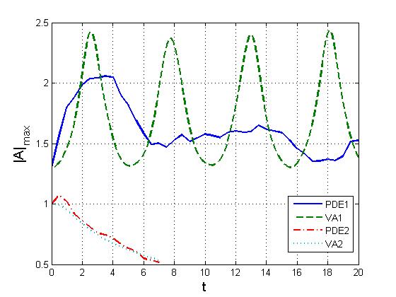
Figure 4: (Color online) Comparison of the evolution  of the soliton’s amplitude, as predicted by the variational approximation (“VA”) and found from direct simulations of the partial differential equation (1) (“PDE”), for $N=5.4$ (a stable soliton) and $N=4.6$ (a decaying state).

The VA predicts eigenfrequency $\omega_{0}$ of intrinsic oscillations of  the weakly perturbed 2D soliton trapped in the static OL, see Eq. (9). Because this feature may be important to understand the response of the soliton to the periodic time modulation of the lattice, in terms of possible resonances (see below), it is necessary to check whether the presence of the eigenfrequency is confirmed by simulations of full equation (1) with the static lattice, i.e., $\varepsilon=0$. To this end, in Fig. 5 we display the power spectrum of small oscillations around the soliton caused by the addition of a small random perturbation to it, for $V_{0}=0.25$ and $N=5.31$, which corresponds to $1-N/\tilde{N}_{\max}\approx\allowbreak 0.155$. As mentioned above, in this case Eqs. (8) and (9) predict the eigenfrequency to be $\omega_{0}\approx 1.35$. The spectrum in Fig. 5 clearly shows the main peak quite close to this point. Peaks corresponding to higher-order resonances (see above) can also be recognized in the figure. To produce the spectrum shown in Fig.5, we simulated the evolution of the soliton up to a very long time, $t=1200$, eliminating a contribution from a relatively short initial stage, which featured a transient behavior.

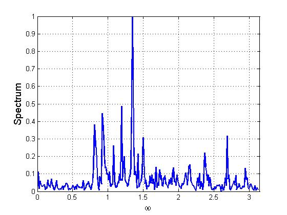
Figure 5: (Color online) The power spectrum of small random perturbations around the stable soliton trapped in the static lattice ($\varepsilon=0$), for $V_{0}=0.25$ and $N=5.31$.

IV.3 Stability diagrams

Results produced by the systematic numerical analysis of the stability of the 2D soliton under the action of the “lattice management” are collected in Fig. 6(a), which displays the stability region in the plane of the modulation parameters, $\omega$ and $\varepsilon$, for fixed $V_{0}=0.25$ and $N=5.905$. Note that this norm again (like in the cases of Figs. 1 and 2) slightly exceeds the collapse threshold in the static model, which is given by Eq. (7). The stability region in the plane of $\varepsilon$ and $N$, for the same OL strength, $V_{0}=0.25$, as in Fig. 6, and $\omega=4$, is displayed in Fig. 6(b). The latter plot explicitly demonstrates the growth of the collapse threshold, $N_{\max}$, with the increase of the modulation amplitude. Note that not the entire parameter region below the stability border in Fig. 6(b) corresponds to stable solitons; if $N$ is too small, the solitons are unstable against decay, see below.

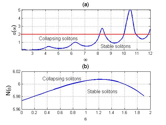
Figure 6: (Color online) (a) The stability region in the plane of the modulation parameters, $\omega$ and $\varepsilon$, for $V_{0}=0.25$ and $N=5.905$. The area relevant to the model with the periodically modulated optical lattice corresponds to $\varepsilon\leq 2$, where the time-dependent amplitude in Eq. (1), $1+\left(\varepsilon/2\right)\cos(\omega t)$, does not change its sign. (b) The collapse threshold versus the modulation amplitude,$\ \varepsilon$, for $V_{0}=0.25$ and $\omega=4$.

In Fig. 6(a), the horizontal line denotes the maximum possible value of the modulation amplitude in the model of the time-modulated OL, $\varepsilon_{\max}=2$. A noteworthy fact is that the stability region can extend up to this limit, i.e., $100\%$ modulation depth (recall that, in the case when the stabilization of 2D solitons was provided by the quasi-1D lattice, the stability limit corresponded to shallow modulation Thawatchai2 ). The results for $\varepsilon>2$ are included too in Fig. 6(a), as they may find a different physical realization, corresponding to a superposition of moving OLs Staliunas:2007a (as mentioned above).

A feature obvious in Fig. 6(a) is a resonant-like dependence of the stability border on $\omega$. This may be a manifestation of the fundamental resonance at $\omega$ close to $\omega_{0}$ and higher-order resonances at multiple values of $\omega$. As argued above, the resonance may help to arrest the collapse, by forcing the vibrating soliton to spend less time in the state where it is “dangerously” narrow. Since the value of the norm corresponding to Fig. 6(a) is close to $N_{\max}$, one may expect that the corresponding fundamental-resonance frequency should be close to one given by Eq. (10), i.e., $\omega_{0}=2$, for $V_{0}=0.25$ [the same is given by Eqs. (8) and (9) in the limit of $N/\tilde{N}_{\max}\rightarrow 0$]. Indeed, the picture in Fig. 6(a) is consistent with the expectation of the fundamental and higher-order resonances at $\omega=n\omega_{0}$, $n=1,2,3,4$ (the picture also suggests the existence of a very strong resonance close to $\omega=5\omega_{0}$, but that one falls deeply into the unphysical region, $\varepsilon>2$).

As mentioned above, the soliton whose norm is too small cannot stabilize itself and decays into quasi-linear waves. Therefore, along with the upper stability boundary, $N=N_{\max}$, that guarantees the absence of the collapse, it is necessary to identify the lower one, $N=N_{\min}$, which secures the stability of the soliton against the decay. Both boundaries, as predicted by the VA and found from the direct simulations, are displayed in Fig. 7, in the form of dependences $N_{\max}(V_{0})$ and$\ N_{\min}(V_{0})$, at fixed $\varepsilon=0.5$ for several different values of $\omega$. In each panel, the stability region is $N_{\min}<N<N_{\max}$.

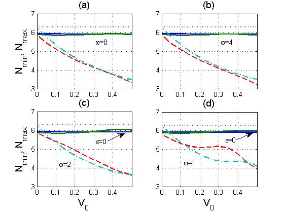
Figure 7: (Color online) The dependence of the stability boundaries, $N_{\max}$ and $\ N_{\min}$, on the OL strength, $V_{0}$, at $\varepsilon=0.5$ and different values of the modulation frequency, $\omega$. Solid and dashed lines show, severally, $N_{\max}$ and $N_{\min}$ as found from the simulations, while the dotted and dashed-dotted lines represent, respectively, $N_{\max}$ and $N_{\min}$ as predicted by the variational approximation. The arrows in (c) and (d) indicate values $N_{\max}$  for the stationary case, $\varepsilon=0$.

We observe in Fig. 7 that dependences $N_{\min}(V_{0})$ produced by the VA are in reasonable agreement with the results of direct simulations of the GPE for modulation frequencies $\omega\geq 2$. However, there is a conspicuous discrepancy between the VA and GPE for $\omega$ close to $1$. On the other hand, this range features strong resonances in the perturbation spectrum, see Fig. 5. Therefore, it is interesting to explore the $N_{\min}(V_{0})$ dependence in region $0.5<\omega<2$, where the resonances may lead to decay of the soliton. These results are displayed in Fig. 8, which shows that plots $N_{\min}(V_{0})$ essentially differ, in this region, from their counterparts both in the static model (see the curve for $\varepsilon=0$ in Fig. 8) and in the high-frequency region, $\omega\geq 2$: actually, $N_{\min}$ increases due to the resonant decay of the solitons. The fact that the resonances are narrow enough, as seen in Fig. 5, may explain a non-monotonous character of dependences $N_{\min}(V_{0})$ for $\omega=1.10$ and $1.25$.

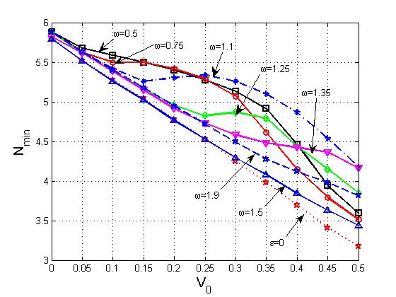
Figure 8: (Color online) Dependencies $N_{\min}(V_{0})$ for $\varepsilon=0.5$ and different modulation frequencies $\omega$ in the resonant area, $0.5<\omega<2$ (see details in text). The curve pertaining to $\varepsilon=0$ (the static model) is included for comparison.

Further, dependences of $N_{\max}$ and $N_{\min}\ \allowbreak$on the modulation frequency are displayed in Fig. 9, for the same modulation amplitude as above, $\varepsilon=0.5$, and several different values of $V_{0}$. It is quite natural that dependences $N_{\min}(\omega)$, as predicted by the VA and generated by direct simulations of Eq. (1), are close to each other for smaller values of the OL strength, $V_{0}=0.1$ and $0.25$, while at $V_{0}=0.5$ the discrepancy between them is considerable. Note non-monotonous behavior of $N_{\min}(\omega)$ in resonant zone $0.5<\omega<2$, which correlates to peculiarities of dependences $N_{\min}(V_{0})$ in the same zone, cf. Fig. 8

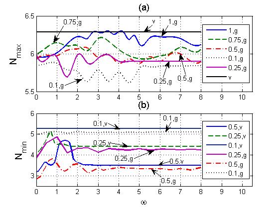
Figure 9: (Color online) The dependence of the upper (a) and lower (b) stability boundaries, $N_{\max}$ and $N_{\min}$, on modulation frequency $\omega$ for $\varepsilon=0.5$ and different values of OL strength $V_{0}$, which are specified in the box. Labels “v” and “g” pertain, severally, to the curves predicted by the variational approximation and those found from direct simulations of Gross-Pitaevskii equation (1) (the VA predicts flat value $\tilde{N}_{\max}=2\pi$, see text). The arrows identify those curves which may seem indisnguishable in the black-and-white rendition of the figure.

V Conclusions

We have studied the dynamics of 2D solitons in the model of BEC trapped in the square-shaped OL (optical lattice) whose strength it subject to the periodic time modulation. Being quite feasible for the experimental implementation, the model belongs to a broad class of schemes of the periodic management of solitons book . By means of the VA (variational approximation) and direct systematic simulations of the underlying Gross-Pitaevskii equation, we have identified stability regions for the solitons in the parameter space of the model, including both maximum and minimum values of the norm, as summarized in Figs. 6, 7, 8 and 9. A remarkable feature demonstrated by these results is that the stability limit may reach the maximum ($100\%$) modulation depth. It is noteworthy too that an increase of the collapse threshold in predicted in comparison with its classical value in the static situation, which corresponds to the norm of the Townes soliton. The stability borders predicted by the VA are found to be in reasonable agreement with the numerical results. In the plane of the modulation frequency and amplitude, the stability boundary features a salient resonant structure, which may also be qualitatively explained by means of the VA. In particular, the minimum norm necessary for the stability of the soliton demonstrates strong variations in the region of low modulation frequencies, due to the possibility of the decay of the soliton enhanced by the resonance.

The analysis reported in this work can be extended in several directions. It may be interesting to study interactions between the solitons in this setting, and identify stability limits for vortex solitons, as well as for 2D gap solitons in the model combining the repulsive nonlinearity and lattice management. Another extension may be made in the direction of an anisotropic lattice management, i.e., applying time modulations shifted by $\pi$ to the two 1D sublattices.

References

- (1) B. A. Malomed, D. Mihalache, F. Wise, and L. Torner, J. Optics B: Quant. Semics. Opt. 7, R53 (2005).
- (2) K. E. Strecker, G. B. Partridge, A. G. Truscott, and F. G. Hulet, Nature 417, 150 (2002); L. Khaykovich, F. Schreck, G. Ferrari, T. Bourdel, J. Cubizolles, L. D. Carr, Y. Castin, and C. Salomon, Science 296, 1290 (2002); S. L. Cornish, S. T. Thompson, and C. E. Wieman, Phys. Rev. Lett. 96, 170401 (2006).
- (3) B. B. Baizakov, B. A. Malomed, and M. Salerno, Europhys. Lett. 63, 642 (2003); J. Yang and Z. H. Musslimani, Opt. Lett. 28, 2094 (2003).
- (4) B. B. Baizakov, B. A. Malomed and M. Salerno, Phys. Rev. A 70, 053613 (2004).
- (5) B. B. Baizakov, B. A. Malomed and M. Salerno, in: Nonlinear Waves: Classical and Quantum Aspects, ed. by F. Kh. Abdullaev and V. V. Konotop, pp. 61-80 (Kluwer Academic Publishers: Dordrecht, 2004); also available at http://rsphysse.anu.edu.au/~asd124/Baizakov_2004_61_NonlinearWaves.pdf.
- (6) J. Kasprzak, M. Richard, S. Kundermann, A. Baas, P. Jeambrun, J. M. J. Keeling, F. M. Marchetti, M. H. Szymanska, R. Andre, J. L. Staehli, V. Savona, P. B. Littlewood, B. Deveaud, and L. S. Dang, Nature 443, 409 (2006).
- (7) D. Mihalache, D. Mazilu, F. Lederer, Y. V. Kartashov, L.-C. Crasovan, and L. Torner, Phys. Rev. E 70, 055603(R) (2004).
- (8) O. Zobay, S. Pötting, P. Meystre, and E. M. Wright, Phys. Rev. A 59, 643 (1999); F. Kh. Abdullaev, B. B. Baizakov, S. A. Darmanyan, V. V. Konotop, and M. Salerno, ibid. 64, 043606 (2001); A. Trombettoni, and A. Smerzi, Phys. Rev. Lett. 86, 2353 (2001); G. L. Alfimov, V. V. Konotop, and M. Salerno, Europhys. Lett. 58, 7 (2002).
- (9) K. M. Hilligsøe, M. K. Oberthaler, and K.-P. Marzlin, Phys. Rev. A 66, 063605 (2002); D. E. Pelinovsky, A. A. Sukhorukov, and Y. S. Kivshar, Phys. Rev. E 70, 036618 (2004).
- (10) B. Eiermann, Th. Anker, M. Albiez, M. Taglieber, P. Treutlein, K.-P. Marzlin, and M. K. Oberthaler, Phys. Rev. Lett. 92, 230401 (2004).
- (11) O. Morsch, M. Oberthaler, Rev. Mod. Phys. 78, 179215 (2006).
- (12) B. B. Baizakov, V. V. Konotop, and M. Salerno, J. Phys. B: At. Mol. Opt. Phys. 35, 5105 (2002); P. J. Y. Louis, E. A. Ostrovskaya, C. M. Savage, and Y. S. Kivshar, Phys. Rev. A 67, 013602 (2003); E. A. Ostrovskaya and Y. S. Kivshar, Opt. Exp. 12, 19 (2004); Phys. Rev. Lett. 93, 160405 (2004); H. Sakaguchi and B. A. Malomed, J. Phys. B 37, 2225 (2004); A. Gubeskys, B. A. Malomed, I. M. Merhasin, Phys. Rev. A 73, 023607 (2006).
- (13) B. B. Baizakov, B. A. Malomed, and M. Salerno, Eur. Phys. J. D 38, 367 (2006).
- (14) H. Sakaguchi, B. A. Malomed, Phys. Rev. E 74, 026601 (2006).
- (15) P. Pedri and L. Santos, Phys. Rev. Lett. 95, 200404 (2005).
- (16) I. Tikhonenkov, B. A. Malomed, and A. Vardi, Phys. Rev. Lett. 100, 090406 (2008).
- (17) H. Saito and M. Ueda, Phys. Rev. Lett. 90, 040403 (2003); F. Kh. Abdullaev, J. G. Caputo, R. A. Kraenkel, and B. A. Malomed, Phys. Rev. A 67, 013605 (2003); G. D. Montesinos, V. M. Pérez-García, and H. Michinel, Phys. Rev. Lett. 92, 133901 (2004).
- (18) I. Towers and B. A. Malomed, J. Opt. Soc. Am. 19, 537 (2002).
- (19) K. Staliunas, S. Longhi, and G. J. de Valcárcel, Phys. Rev. A 70, 011601(R) (2004).
- (20) M. Trippenbach, M. Matuszewski, and B. A. Malomed, Europhys. Lett. 70, 8 (2005); M. Matuszewski, E. Infeld, B. A. Malomed, and M. Trippenbach, Phys. Rev. Lett. 95, 050403 (2005).
- (21) V. A. Brazhnyi and V. V. Konotop, Phys. Rev. A 72, 033615 (2005); M. A. Porter, M. Chugunova and D. E. Pelinovsky, Phys. Rev. E 74, 036610 (2006).
- (22) P. G. Kevrekidis, G. Theocharis, D. J. Frantzeskakis, and B.A. Malomed, Phys. Rev. Lett. 90, 230401 (2003).D. E. Pelinovsky, P. G. Kevrekidis, and D. J. Frantzeskakis, ibid. 91, 240201 (2003); F. Kh. Abdullaev, R. M. Galimzyanov, M. Brtka, and R. A Kraenkel, J. Phys. B: At. Mol. Opt. Phys. 37 (2004) 3535 (2004).
- (23) B. A. Malomed. Soliton Management in Periodic Systems (Springer: New York, 2006).
- (24) A. Itin, T. Morishita, and S. Watanabe, Phys. Rev. A 74, 033613 (2006).
- (25) C. Tozzo, M. Krämer, and F. Dalfovo, Phys. Rev. A 72, 023613 (2005); M. Krämer, C. Tozzo, and F. Dalfovo, Phys. Rev. A 71, 061602(R) (2005).
- (26) T. Mayteevarunyoo and B. A. Malomed, Phys. Rev. A 74, 033616 (2006).
- (27) C. Schori, T. Stöferle, H. Moritz, M. Köhl, and T. Esslinger, Phys. Rev. Lett. 93, 240402 (2004).
- (28) J. J. G. Ripoll and V. M. Pérez-García, Phys. Rev. A 59, 2220 (1999); J. J. García-Ripoll, V. M. Pérez-García, and Pedro Torres, Phys. Rev. Lett. 83, 1715 (1999); B. Baizakov, G. Filatrella, B. Malomed, and M. Salerno, Phys. Rev. E 71, 036619 (2005); P. Engels, C. Atherton, and M. A. Hoefer, Phys. Rev. Lett. 98, 095301 (2007); Yu. Kagan and L. A. Manakova, Phys. Rev. A 76, 023601 (2007).
- (29) K. Staliunas, S. Longhi, and G. J. de Valcárcel, Phys. Rev. Lett. 89, 210406 (2002); Phys. Rev. A 70, 011601(R) (2004).
- (30) P. Engels, C. Atherton, and M. A. Hoefer, Phys. Rev. Lett. 98, 095301 (2007).
- (31) H. Saito, R. G. Hulet, and M. Ueda, Phys. Rev. A 76, 053619 (2007); H. Susanto, G. K. Kevrekidis, B. A. Malomed, and F. Kh. Abdullaev, Phys. Lett. 372, 1631 (2008).
- (32) T. Mayteevarunyoo, B. A. Malomed, and M. Krairiksh, Phys. Rev. A 76, 053612 (2007).
- (33) K. Staliunas, R. Herrero, and G. J. de Valcárcel, Phys. Rev. A 75, 011604(R) (2007).
- (34) K. Staliunas, R. Herrero, and G. J. de Valcárcel, Phys. Rev. E 73, 065603(R) (2006).
- (35) G. Burlak and A. Klimov, Phys. Lett. A 369, 510 (2007).
- (36) B. B. Baizakov and M. Salerno, Phys. Rev. A 69, 013602 (2004).
- (37) M. Desaix, D. Anderson, M. Lisak, J. Opt. Soc. Am. B 8, 2082 (1991).
- (38) V. M. Pérez-García, H. Michinel, J. I. Cirac, M. Lewenstein, and P. Zoller, Phys. Rev. A 56, 1424 (1997); B. A. Malomed, in Progress in Optics, vol. 43, p. 71, ed. by E. Wolf (Amsterdam: North-Holland, 2002).
- (39) L. Bergé, Phys. Rep. 303, 259 (1998).
- (40) L. D. Landau and E. M. Lifshitz, Mechanics, 3rd ed. (Pergamon Press: Oxford, England, 1976).
- (41) F. Kh. Abdullaev and J. G. Caputo, Phys. Rev. E 58, 6637 (1998).
- (42) W. H. Press, S. A. Teukovsky, W. T. Vetterling, and B. P.Flannery, Numerical recipes in C++ (Cambridge University Press: Cambridge, 2002).
- (43) W. L. Kath and N. F. Smyth, Phys. Rev. E 51, 1484 (1995).