The Behavior of the Aromatic Features in M101 HII Regions: Evidence for Dust Processing

Abstract

The aromatic features in M101 were studied spectroscopically and photometrically using observations from all three instruments on the Spitzer Space Telescope. The global SED of M101 shows strong aromatic feature (commonly called PAH feature) emission. The spatially resolved spectral and photometric measurements of the aromatic feature emission show strong variations with significantly weaker emission at larger radii. We compare these variations with changes in the ionization index (as measured by [NeIII]/[NeII] and [SIV/SIII], which we probe over the ranges 0.03–20 and 0.044–15 respectively) and metallicity (expressed as log(O/H) + 12, which ranges from 8.1 to 8.8). Over these ranges, the spectroscopic equivalent widths of the aromatic features from 7 HII regions and the nucleus were found to correlate better with ionization index than with metallicity. This implies that the weakening of the aromatic emission in massive star forming regions is due primarily to processing of the dust grains in these environments, not to differences in how they form (although formation could still be important on a secondary basis). The behavior of the correlation between the aromatic feature equivalent widths and ionization index can be described as a constant equivalent width until a threshold in ionization index is reached ([NeIII]/[NeII] $\sim 1$), above which the equivalent widths decrease with a power law dependence. This behavior for M101 HII regions is also seen for the sample of starburst galaxies presented in the companion study of Engelbracht et al. (2008) which expands the range of [NeIII]/[NeII] ratios to 0.03–25 and log(O/H)+12 values to 7.1–8.8. The form of the correlation explains seemingly contradictory results present in the literature. The behavior of the ratios of different aromatic features versus ionization index does not follow the predictions of existing PAH models of the aromatic features implying a more complex origin of the aromatic emission in massive star forming regions.

1. Introduction

The interpretation of infrared measurements of star forming galaxies rests on an understanding of the properties of the dust producing the emission. In addition, the dependence of dust properties on environment provides important clues to the dust composition and formation. An important constituent of the interstellar dust is large, aromatic molecules/grains whose emission often dominates the mid-infrared output of HII regions and galaxies (Roche et al., 1991; Madden et al., 2006; Smith et al., 2007b).

The aromatic features were first discovered in observations of planetary nebulae where a feature at 11.3 µm was broader than the observed atomic emission lines (Gillett et al., 1973). The number of these features has grown to include many features with wavelengths between 3 and 18 µm (Werner et al., 2004; Smith et al., 2004; Tielens, 2005). The strongest aromatics are seen at 3.3, 6.2, 7.7, 8.6, 11.3, 12.7, and 17.1 µm and all the aromatics have been identified with C-H and C-C bending and stretching modes of hydrocarbons containing aromatic rings (Tielens, 2005). The shape and strength of the aromatics have been seen to vary in single sources (Werner et al., 2004), among various Galactic sources (van Diedenhoven et al., 2004), and among galaxies (Engelbracht et al., 2005; Madden et al., 2006; Wu et al., 2006).

A number of different materials have been proposed as the carriers of these features, including Hydrogenated Amorphous Carbon (HAC, Duley & Williams, 1983), Quenched Carbonaceous Composites (QCC, Sakata et al., 1984), Polycyclic Aromatic Hydrocarbons (PAHs, Allamandola et al., 1985), coal (Papoular et al., 1989), and nanodiamonds (Jones & d’Hendecourt, 2000). The leading candidate material for the aromatics is PAH molecules and they are often included in the modified “astronomical PAHs” form in dust grain models (Li & Draine, 2001; Zubko et al., 2004). We refer to these features as the aromatic features to allow for discussions of the observations without making an assumption about the material that is responsible for them. We refer the interested reader to Peeters et al. (2004) for a detailed discussion of these features.

The observed strengths of the aromatic features do not vary much in most normal luminosity galaxies with approximately solar metallicities (Roche et al., 1991; Lu et al., 2003; Smith et al., 2007b) or massive starbursts (Brandl et al., 2006). The strength of these features do weaken significantly in active galactic nuclei (Roche et al., 1991; Lutz et al., 1998; Smith et al., 2007b) and star bursting galaxies with fairly low metallicities (Roche et al., 1991; Engelbracht et al., 2005; Galliano et al., 2005; Madden et al., 2006; Wu et al., 2006; Engelbracht et al., 2008). The variations seen in active galactic nuclei are not considered for this paper, which only discusses those clearly associated with nearby massive star formation (e.g., starburst galaxies and HII regions). Observations with the Infrared Space Observatory (ISO) found that the strength of the aromatic features was correlated with a galaxy’s metallicity (probed by log(O/H)+12) and ionization (probed by [NeIII]/[NeII]), but were unable to determine which was the dominant effect (Madden et al., 2006). The correlations are such that the aromatic features are weakest for low metallicities and high ionizations.

If the correlation is better with metallicity than ionization, then this implies that the formation of the aromatics (from the constituent atoms in circumstellar or interstellar environments) happens less efficiently than that of small grains as the metallicity decreases. On the other hand, if the better correlation is with ionization, then this implies that there is increased processing of the aromatic feature carriers (modification and/or destruction in the immediate environment) as the radiation field becomes harder. Throughout this paper, we use the metallicity as a probe of the formation of aromatics from the constitute atoms and ionization as a probe of the processing of the aromatics in the immediate environment. The metallicity and ionization in massive star forming regions is roughly correlated making it nontrivial to determine which is the dominate correlation.

Observations with Spitzer have refined the observational picture of the variations of the aromatic features among galaxies, but have yet to provide a clear picture of the origin of the variations. Evidence that the aromatic features are absent at the lowest metallicities probed by starburst galaxies was provided by the IRS (Infrared Spectrograph) spectrum of SBS 0335-052 which has a log(O/H)+12=7.2 (Houck et al., 2004a). The weakness/absence of aromatic features at metallicities below log(O/H)+12=8.2 in a sample of starburst galaxies was shown by Engelbracht et al. (2005) using IRAC (Infrared Camera) and MIPS (Multiband Imaging Photometry for Spitzer) photometry confirmed in a few cases with IRS spectroscopy. Wu et al. (2006) studied a small sample of Blue Compact Dwarf galaxies (including SBS 0335-052) with IRS spectroscopy and found similar correlations between aromatic feature equivalent width and metallicity or radiation field hardness. Brandl et al. (2006) found that the equivalent width of the aromatic features did not vary significantly over a factor of 10 in [NeIII]/[NeII] for a sample of starburst galaxies. Using the HII classified galaxies in the SINGS (Spitzer Nearby Galaxies Survey) sample Smith et al. (2007b) found variations in the summed strength of the aromatic features when ratioed to the total IR flux with some indication of a threshold at log(O/H)+12=8.1. The metallicity threshold in the aromatic feature strengths was confirmed by Draine et al. (2007) where the broadband spectra energy distributions (SEDs) of the SINGS galaxies were modeled. These models indicated a fairly abrupt reduction by a factor of three occurs in the fraction of PAHs near a metallicity of log(O/H)+12 = 8.1.

All this variation among galaxies raises the question: do the aromatics vary significantly among HII regions in a single galaxy? The study of the simpler environments of HII regions may also present a clearer picture of the cause of the aromatic feature variations as HII regions have much more homogeneous physical conditions than whole galaxies. The ideal galaxy to answer this question is the giant spiral galaxy M101. M101 is a large ($>30$′diameter), face-on spiral galaxy (SABcd) at a distance of 6.7 Mpc (Freedman et al., 2001). It has one of the largest metallicity gradients known with metallicities [log(O/H) + 12] ranging from 8.8 in the nucleus to 7.4 in an HII region 41 kpc from the center (Zaritsky et al., 1994; van Zee et al., 1998; Kennicutt et al., 2003a; Bresolin, 2006). In addition, there are high quality electron temperature and metallicity determinations for a sample of M101 HII regions with metallicities from 7.4 to 8.8 (Kennicutt et al., 2003a; Bresolin, 2006). This large apparent size, the numerous HII regions, the large metallicity gradient, and the high quality metallicity measurements make M101 ideal for studying the dependence of the aromatics on the local conditions, specifically metallicity and ionization.

2. Data

The high sensitivity and spatial resolution provided by all three instruments on Spitzer allow individual HII regions in M101 to be studied in detail. Targeted spectroscopic observations of a handful of HII regions and the nucleus were taken with the Infrared Spectrograph (IRS, Houck et al., 2004b). Imaging of M101 was obtained with the Infrared Array Camera (IRAC, Fazio et al., 2004) at 3.6, 4.5, 5.8, 8.0 µm and the Multiband Imaging Photometry for Spitzer (MIPS, Rieke et al., 2004) at 24, 70, and 160 µm. The IRAC and MIPS images allow the general behavior of the aromatics to be studied over the entire galaxy and the IRS spectra allow for the behavior of the aromatics to be probed in detail for selected HII regions. Past studies of M101 in the infrared have concentrated on radial gradients as the spatial resolution was not high enough to study any but the few brightest HII regions (eg. Hippelein et al., 1996; Popescu et al., 2005).

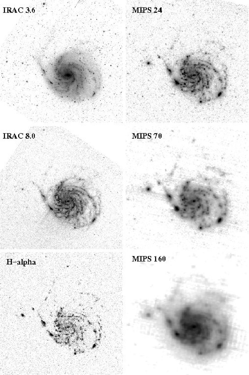
Figure 1.— IRAC, MIPS, and H$\alpha$ images of M101 at full resolution. The IRAC 4.5 and 5.8 µm images have not been shown as they look very similar to the IRAC 3.6 and 8.0 µm images, respectively. The field-of-view of the images is $30\arcmin\times 30\arcmin$. The H$\alpha$ image (van Zee et al., 1998) is included to show the locations of HII regions. The streaking seen SE of M101 at 8 µm and roughly East-West at 70 and 160 µm are residual instrumental artifacts.

Preliminary results from the IRAC and MIPS images were presented by Gordon et al. (2006b) and from the IRS spectroscopy in Gordon et al. (2006a). This work focuses on the intense star forming HII regions in a single galaxy and is complementary to the Spitzer program on starburst galaxies led by Charles Engelbracht (Engelbracht et al., 2005, 2006, 2008) which focuses on the properties whole galaxies undergoing intensive star formation.

2.1. IRAC and MIPS Images

The IRAC images of M101 were obtained on 8 March 2004. Two maps were taken separated by a few hours to allow for asteroid rejection. Each map consisted of $13\times 13$ tiles with 150″offsets (1/2 the array width) between tile positions in both array dimensions . Each exposure was taken in high dynamic range (HDR) mode resulting in two images, one with a 10.4 sec exposure time and one with a 0.4 second exposure time. The images were reduced with the Spitzer Science Center (SSC) pipeline S13.2.0 and combined using MOPEX program (v030106). As part of the mosaicking, overlapping regions of adjacent images were used to correct for bias drifts in each image. The calibration of the images was corrected to an infinite aperture (true surface brightness units) using the values given by Reach et al. (2005). The final mosaics have exposure times of $\sim$85 seconds/pixel and are shown in Figure 1.

The MIPS images of M101 were obtained on 10-11 May 2004. Like the IRAC images, two maps were taken separated by a few hours for asteroid rejection. Each map consisted of 14 medium rate 0.75 degree scan legs with a cross scan offset of 148″. We used version 3.06 of the MIPS Data Analysis Tool (DAT) (Gordon et al., 2005) to do the basic processing and final mosaicking of the individual images. Extra processing steps before mosaicking used programs written specifically to improve the reduction of large, well-resolved galaxies. At 24 µm the extra steps included readout offset correction, scan mirror dependent flat fields, array averaged background subtraction (using a low order polynomial fit to the data in each scan leg but excluding M101), and rejection of the 1st 5 images in each scan leg due to bias boost transients. At 70 and 160 µm the extra steps were a pixel dependent background subtraction for each map (using a low order polynomial fit to the data in each scan leg, again excluding M101) and a spatial cosmic ray cleaning (160 µm only). The calibration of the MIPS bands was done using the latest, official factors (Engelbracht et al., 2007; Gordon et al., 2007; Stansberry et al., 2007). The 5$\sigma$ depth achieved in a single beam by these observations is 0.050, 0.53, and 0.74 MJy sr^-1 for beam FWHM of 6$\arcsec$, 18$\arcsec$, and 40$\arcsec$ and exposure times of $\sim$200, $\sim$80, and $\sim$18 seconds/pixel for 24, 70, and 160 µm, respectively. The final mosaics are shown in Figure 1. The streaking seen along the scan direction at 70 & 160 µm is caused by residual instrumental artifacts and only produces a significant worsening of the noise at 70 µm. The online MIPS SENS-PET program predicts approximately the observed noise at 24 & 160 µm  but a factor of 3 lower noise than observed for the 70 µm observations. This difference is likely due to the residual streaking seen along the scan mirror direction which can be suppressed by combining scan maps taken at different scan angles (Tabatabaei et al., 2007). Additional MIPS scan maps of M101 are planned and will be the subject of a future paper.

Figure 2.— A 3 color image of M101 is shown annotated with the locations of HII regions with measured metallicities. The red, green, and blue channels are filled with the MIPS 24 µm, IRAC 8 µm, and IRAC 3.6 µm images, respectively. The regions that were observed with IRS are identified as having a box around their names.

2.2. IRS Spectra

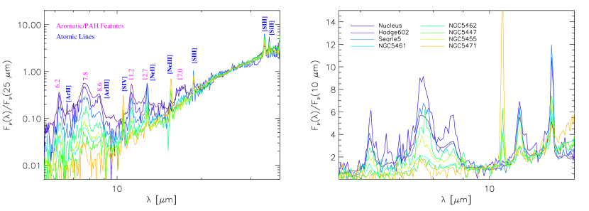
Figure 3.— The IRS spectrum for all 8 regions with targeted IRS spectroscopy are shown. The left plot show the full spectra normalized to their average flux in the 20–30 µm region and on a log scale. The locations of aromatic and atomic emission lines are given. The right plot shows the 5–15 µm portion of the spectra normalized to their average flux at 10 µm and on a linear scale. The legend identifying the regions is given in this plot.

Table 1M101 Regions with measured metallicities

Name	Other Names	Coordinates	R/Ro	12+log(O/H)	IRS Spectra
Nucleus		14 03 12.48 54 20 55.4	0.00	$8.76\pm 0.06$	X
Hodge 602		14 03 10.22 54 20 57.8	0.02	$8.76\pm 0.06$	X
Hodge 1013		14 03 31.39 54 21 14.5	0.19	$8.71\pm 0.05$
Searle 5	Hodge 336	14 02 55.05 54 22 26.6	0.21	$8.55\pm 0.16$	X
NGC 5461	Hodge 1105	14 03 41.36 54 19 04.9	0.32	$8.50\pm 0.03$	X
NGC 5447	Hodge 128	14 02 28.18 54 16 26.3	0.55	$8.45\pm 0.04$	X
NGC 5462	Hodge 1170	14 03 53.19 54 22 06.3	0.44	$8.37\pm 0.07$	X
NGC 5455	Hodge 409	14 03 01.13 54 14 28.7	0.46	$8.25\pm 0.03$	X
Hodge 67		14 02 19.92 54 19 56.4	0.54	$8.14\pm 0.08$
Hodge 70/71		14 02 20.50 54 17 46.0	0.57	$8.10\pm 0.12$
Searle 12	Hodge 1216	14 04 11.11 54 25 17.8	0.67	$8.16\pm 0.03$
NGC 5471	NGC 5471-D	14 04 29.35 54 23 46.4	0.80	$8.09\pm 0.03$	X
Hodge 681		14 03 13.64 54 35 43.0	1.03	$7.92\pm 0.09$

Low resolution IRS spectra from 5-38 µm of 7 HII regions and the nucleus were taken in the spectral mapping mode with full slit width steps perpendicular to the slit. The locations of these 7 regions as well as other HII regions with measured electron temperatures and metallicities from Kennicutt et al. (2003a) are shown in Fig. 2 and their basic details are given in Table 1. The ShortLow spectra (5–15 µm) were taken with 6 steps and the LongLow (15–38 µm) were taken with 2 steps so that both spectral apertures covered the same regions. The metallicities [12+log(O/H)] are taken from table 5 of Kennicutt et al. (2003a) except for the values for the nucleus and Hodge 602, which are the constant term in their equation 5. The ShortLow and LongLow observations were taken approximately 3 months apart so the orientations of the two slits were approximately the same on the sky.

These spectral mapping observations were reduced with the SSC pipeline (version S13/S14) and combined using CUBISM program (Smith et al., 2007a). Spectra were extracted from the cubes for each HII region and the nucleus using an aperture with a radius of 10″ and sky annuli from 12 to 18″ referenced at 24 µm. The size of the aperture and sky annuli were varied linearly with wavelength to account roughly for the changing diffraction limited point-spread-function (PSF), with a minimum object aperture radius of 5″ to account of the finite size of the HII regions. The outlines of the individual IRS slits and extraction apertures are shown in Fig. 4 superimposed on cutouts of the IRAC 8 µm and MIPS 24 µm images centered on each HII region. There are issues of crowding with nearby HII regions for some of the targets, but for the most part the targets are fairly well separated. The measured noise in the sky annuli region was used to compute the uncertainty on each point in the spectrum.

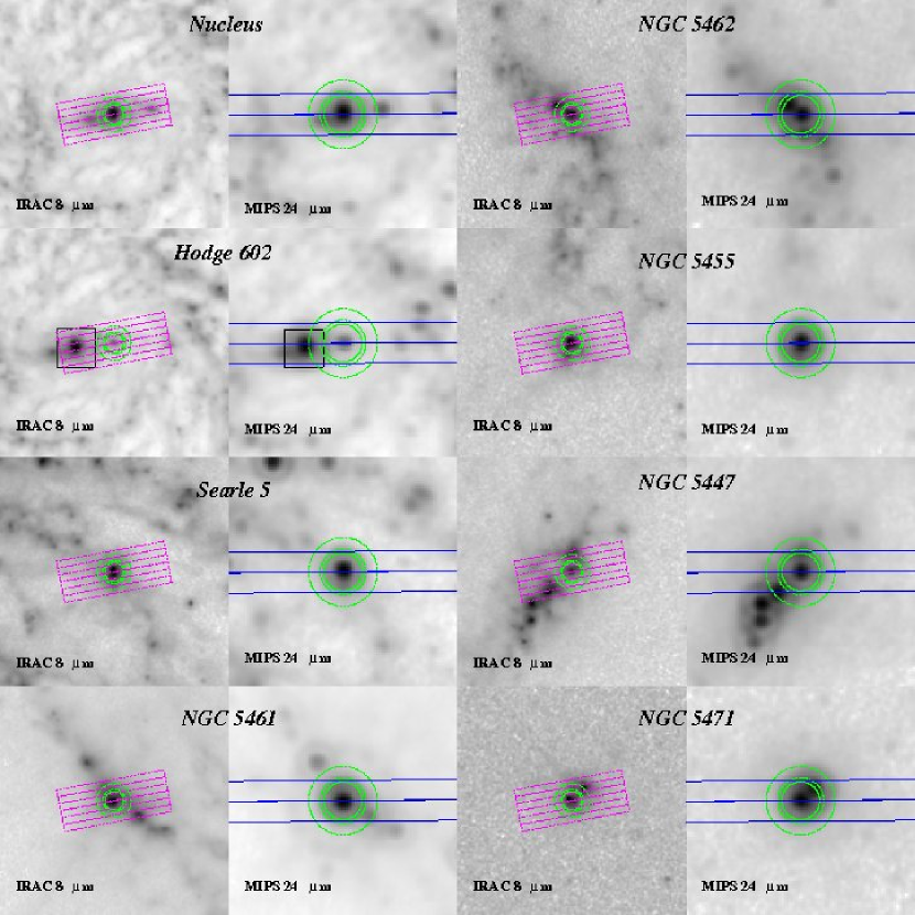
Figure 4.— Cutouts centered on each of the 8 regions with targeted IRS spectroscopy are shown. Each cutout is $2\arcmin\times 2\arcmin$ and shows the circular extraction aperture (and sky annulus) at that wavelength and the outline of the ShortLow and LongLow slits on the IRAC 8 µm and MIPS 24 µm images, respectively. For Hodge 602, the nearby nuclear region was masked (black square shown) to allow for an accurate sky measurement.

The six spectral segments for each target were merged into a single spectrum using the overlap regions to adjust the level of each segment to be consistent. The overall level of the spectra was set by requiring each spectrum to be consistent with the MIPS 24 µm measurement given in Table 3. The main adjustment is at the transition between the ShortLow and LongLow spectra. This is not surprising given the observing strategy where the region is sampled with 6 ShortLow positions, but only 2 LongLow positions. The resulting merged spectra are shown in Fig. 3.

2.3. Resolution Matching

One of the challenges of working with Spitzer data is the large change in PSF with wavelength as Spitzer is diffraction limited at wavelengths longer than $\sim$6 µm. The FWHM (full width half maximum) of the Spitzer PSF varies from around $2\arcsec$ for the IRAC bands to $5\arcsec$, $18\arcsec$, and $40\arcsec$ for the MIPS 24, 70, and 160 µm bands. To allow for accurate comparisons between wavelengths, it is important to convolve all images of interest to the lowest common resolution. Without this step, it is not easy to compare extended sources at different Spitzer bands given that the physical region probed changes with wavelength. The Spitzer PSFs are much more complex than simple Guassians with pronounced Airy rings and diffraction spikes. This makes it definitely non-optimal to use simple Gaussian kernels to achieve the desired common resolution. It is also possible to put a set of images on a common resolution by convolving each image with all the other image PSFs, but this clearly creates a lower resolution common PSF than the method detailed below.

The optimal method in the case of complex PSFs is to construct convolution kernels that transform the input PSF to the desired common resolution PSF. Theoretically, the desired convolution kernel can be constructed using 2D Fast Fourier Transforms (FFTs) and is just

$$K(x,y)=\mathrm{FFT}^{-1}\left\{\frac{\mathrm{FFT}\left[\mathrm{PSF}_{2}(x,y)\right]}{\mathrm{FFT}\left[\mathrm{PSF}_{1}(x,y)\right]}\right\}$$ (1)

where $\mathrm{PSF}_{1}$ is the input image PSF, $\mathrm{PSF}_{2}$ is the desired common resolution PSF, and K is the convolution kernel that transforms $\mathrm{PSF}_{1}$ to $\mathrm{PSF}_{2}$. Unfortunately, the high frequency numeric noise in $\mathrm{PSF}_{1}$ is greatly amplified and the resulting kernel is dominated by noise. The solution is to add a clamping function that attenuates the high frequency noise $\mathrm{FFT}\left[\mathrm{PSF}_{1}(x,y)\right]$. As the dominant signal we are interested in is radial, we adopt a radial Hanning truncation function, $W_{h}(\omega)$, with the form

$$W_{h}(\omega)=\left\{\begin{array}[]{ll}\frac{1}{2}\left[1+\cos\left(\frac{2\pi\omega}{\omega_{o}}\right)\right]&\omega\leq\omega_{o},\\ 0&\omega>\omega_{o}\\ \end{array}\right.$$ (2)

where $\omega$ is radial spatial frequency and $\omega_{o}$ is the cutoff radial spatial frequency (Brigham, 1988). The revised equation for the desired convolution kernel is then

$$K(x,y)=\mathrm{FFT}^{-1}\left\{\frac{\mathrm{FFT}\left[\mathrm{PSF}_{2}(x,y)\right]}{W_{h}(\omega)\mathrm{FFT}\left[\mathrm{PSF}_{1}(x,y)\right]}\right\}.$$ (3)

The value of $w_{o}$ in eq. 2 is chosen to be as large as possible while still suppressing the high frequency noise in $\mathrm{FFT}\left[\mathrm{PSF}_{1}(x,y)\right]$.

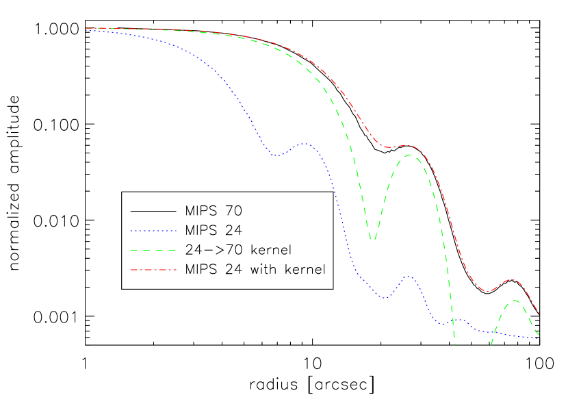
Figure 5.— The radial profiles of the 24 µm PSF, the 24-to-70 µm kernel, the 70 µm PSF, and the convolution of the 24 µm PSF and the 24-to-70 µm kernel are shown.

This method of creating convolution kernels creates a set of images with a common PSF of the lowest resolution in the set. For this method to work, the PSFs of each image have to be known to a reasonable degree and convolution kernels created for each unique PSF in the image set. The value of $\omega_{o}$ is set as large as possible for each kernel by visual inspection of the convolution of $\mathrm{PSF}_{1}(x,y)$ with $K(x,y)$. The goal is for this convolution to reproduce $\mathrm{PSF}_{2}(x,y)$ with the highest possible accuracy while minimizing the noise injected into the operation. An example showing the performance of the 24-to-70 µm convolution kernel is given in Fig. 5. The close (but not perfect) correspondence between the 70 µm PSF and the convolution of the 24 µm PSF with the 24-to-70 µm kernel is a validation of the accuracy of this method.

For the work on M101, we created convolution kernels that transform the IRAC PSFs to the MIPS 24 µm PSF for use in §3.3 and kernels that transform the IRAC, MIPS 24 µm  and MIPS 70 µm PSFs to the MIPS 160 µm PSF for use in §3.4. Ideally, we would have done the same to match the resolutions of each IRS wavelength to the resolution of the longest IRS wavelength. Unfortunately, the IRS PSFs are not nearly as well characterized as the IRAC and MIPS PSFs and our small regions mapped with IRS would introduce significant edge effects in any convolutions. Instead, we varied the extraction apertures to account for the changing IRS PSF with wavelength.

3. Results

With the data presented in this paper, the behavior of the aromatic features in M101 can be probed both photometrically and spectroscopically. The IRAC and MIPS total M101 fluxes are combined with previous measurements to probe the global SED of M101 (§3.1). Using the IRS spectra of the targeted HII regions, we probe the aromatic feature behavior in detail in §3.2. Returning to the imaging data, the behavior of the aromatics for an expanded sample of regions is studied (§3.3) and, finally, the overall infrared morphology is used to gain further insight into the aromatics in M101 (§3.4). Combining both the spectroscopic and photometric approaches produces a richer picture of the aromatic feature behavior than is possible with either approach separately.

3.1. Global SED

The global IR SED of M101 is useful to put this galaxy in context with other galaxies and to probe the overall aromatic and dust content. The IRAC and MIPS global fluxes were measured using a circular aperture with a radius of $13\farcm 3$ and a sky annulus from $14\farcm 2$ to $16\farcm 7$. The uncertainties on these fluxes are dominated by the uncertainties in the absolute calibrations. The IRAC absolute calibration uncertainties are taken as 5% which is larger than the point source uncertainty of $\sim$2% (Reach et al., 2005) as the IRAC scattered light behavior makes the extended source calibration less accurate. The MIPS absolute uncertainties are 4% (Engelbracht et al., 2007), 5% (Gordon et al., 2007), and 12% (Stansberry et al., 2007). We have tabulated previous IR measurements of the total M101 emission in Table 3.1. We have included the ISOPHOT (Lemke et al., 1996) flux from Stickel et al. (2004) but not the fluxes given by Tuffs & Gabriel (2003) as these fluxes are known to be lower limits. The Midcourse Space Experiment (MSX, Cohen et al., 2001) observed M101 in four mid-infrared bands (Kraemer et al., 2002), but only had a high signal-to-noise detection in MSX Band A. The MSX Band A flux was measured using the same apertures as the IRAC and MIPS fluxes from the image available from NED. The uncertainty on this measurement was set to 20% to account for the difficulty in sky subtraction for these data.

Table 2M101 Global Fluxes

	Wavelength	Bandwidth	Flux
Band	[µm]	[µm]	[Jy]	Origin	Reference
J	1.235	0.162	$3.94\pm 0.12$	2MASS	1
H	1.662	0.251	$4.88\pm 0.19$	2MASS	1
K	2.159	0.262	$4.16\pm 0.20$	2MASS	1
IRAC1	3.550	0.681	$2.84\pm 0.14$	Spitzer/IRAC	2
IRAC2	4.493	0.872	$1.76\pm 0.09$	Spitzer/IRAC	2
IRAC3	5.731	1.250	$3.69\pm 0.18$	Spitzer/IRAC	2
LW2	6.75	3.5	$6.03\pm 0.442$	ISO/ISOCAM	3
IRAC4	7.872	2.526	$7.26\pm 0.36$	Spitzer/IRAC	2
MSXA	8.276	3.362	$8.86\pm 1.77$	MSX	2
IRAS12	12	7.0	$6.2\pm 0.93$	IRAS	4
COBE12	12	6.48	$<16.9$	COBE/DIRBE	5
LW3	15.0	6.0	$5.42\pm 0.501$	ISO/ISOCAM	3
MIPS24	23.7	4.7	$10.5\pm 0.4$	Spitzer/MIPS	2
IRAS25	25	11.2	$11.8\pm 1.77$	IRAS	4
COBE25	25	8.60	$12.2\pm 2.44$	COBE/DIRBE	5
IRAS60	60	32.5	$88.0\pm 13.2$	IRAS	4
COBE60	60	27.84	$82.8\pm 16.6$	COBE/DIRBE	5
MIPS70	71.0	19.0	$116.3\pm 7.0$	Spitzer/MIPS	2
IRAS100	100	31.5	$252.8\pm 37.9$	IRAS	4
COBE100	100	32.47	$259.0\pm 51.8$	COBE/DIRBE	5
COBE140	140	39.53	$<530.0$	COBE/DIRBE	5
MIPS160	156	35.0	$405.3\pm 35.0$	Spitzer/MIPS	2
ISO170	170	90.2	$495.8\pm 74.4$	ISO/ISOPHOT	6
COBE240	240	95.04	$<497.5$	COBE/DIRBE	5

References. — (1) Jarrett et al. (2003); (2) this work; (3) Roussel et al. (2001); (4) Rice et al. (1988) (5) Odenwald et al. (1998) (6) Stickel et al. (2004)

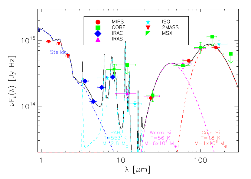
Figure 6.— The IR SED of M101 is shown from the new IRAC and MIPS observations presented here as well as measurements taken from the literature. The COBE/DIRBE upper limits are 3$\sigma$. The horizontal error bars give the widths of the bands. A simple stellar population plus 3 component dust emission model fit is shown. Each dust component is modeled with a single grain size and the temperature given is the equilibrium temperature. The PAH component is illustrative only as it is assumed to be in thermal equilibrium which is an approximation as this component is known to be heated stochastically.

The global IR SED of M101 is shown in Fig. 6 and looks similar to many of the Spitzer Nearby Galaxies Survey Kennicutt et al. (2003b, SINGS,) galaxy global SEDs (Dale et al., 2005, 2007; Draine et al., 2007). We fit the global SED of M101 with the combination of a simple stellar population and a three component dust grain emission model. The details of this modeling can be found in Marleau et al. (2006). While this model is not unique, it is illustrative of the dust properties implied by the SED. The global IR SED of M101 includes strong aromatic emission features as well as emission from warm (T $\sim 56$ K) and cold (T $\sim 18$ K) dust. The total dust mass of $1\times 10^{8}$ M_☉ is dominated by the coldest component and is much larger than the previous estimate of $4.8\times 10^{6}$ M_☉ based on IRAS data alone (Young et al., 1989). Using our new measurement of the dust mass, the M101 gas-to-dust ratio is $\sim$300 using a HI mass of $2.5\times 10^{10}$ M_☉ (Bosma et al., 1981) and a H₂ mass of $5.1\times 10^{9}$ M_☉. This new gas-to-dust ratio is much smaller than the previous measurement of 2440 by Devereux & Young (1990). This is in accordance with their suspicion that there was an order of magnitude more dust which was too cold for IRAS to measure. The dust-to-gas ratio we measure is consistent with that expected for a galaxy with a global metallicity of 8.4 (Kennicutt et al., 2003a; Moustakas & Kennicutt, 2006) from the work of Draine et al. (2007) on SINGS global SEDs.

The global obscured SFR can be measured using the total IR luminosity and the calibration given by Kennicutt et al. (2003a). The total IR luminosity of M101 determined using the TIR (total IR) formulation (Dale & Helou, 2002) is $2.5\times 10^{43}$ ergs s^-1 which gives a SFR of 1.1 $M_{\sun}$ year^-1. The global obscured SFR can also be measured using the MIPS 24 µm luminosity ($\lambda F(24~{}\micron)4\pi d^{2}$, where d = distance) which is $7.05\times 10^{43}$ ergs s^-1. This gives a SFR of 1.8 and 1.1 $M_{\sun}$ year^-1 using the calibrations of Alonso-Herrero et al. (2006) or Calzetti et al. (2007), respectively.

3.2. Spectroscopic Measures of Aromatics

Measuring the strengths of the aromatic features in the IRS spectra is not straightforward given that many of the features are blended with each other as well as with atomic emission lines. Various methods have been used in the past that attempt to define continuum points between features and measure consistently portions of the aromatic features, but these are prone to systematic errors as the level of blending changes with the strength of the features. Fortunately, Smith et al. (2007b) provided a decomposition tool called PAHFIT to fit simultaneously the aromatic features, atomic and molecular emission lines, dust and stellar continuum, and the dust extinction in IRS spectra. Some previous work in this area has used similar fitting techniques (e.g., Madden et al., 2006), but PAHFIT is the first such tool to fit simultaneously all the components of the mid-IR spectra of star forming region. As PAHFIT takes into account the blending of the aromatic and atomic features, it produces fairly precise measurements of their individual strengths. We used the PAHFIT program to fit all of our M101 spectra and the resulting fits for two of the regions are shown in Fig. 7. The atomic emission line strengths from the fits are given in Table 4. The aromatic emission line strengths and equivalent widths are given in Tables 5 and 6, respectively. The line strengths are computed by integrating the fit profile for the specific line and does not include any contribution to the continuum. The equivalent width is

$$\int\left(\frac{I(\nu)-I(\nu)_{\mathrm{cont}}}{I(\nu)_{\mathrm{cont}}}\right)\delta\lambda$$ (4)

where $I(\nu)=I(\nu)_{\mathrm{line}}+I(\nu)_{\mathrm{cont}}$ (both from the PAHFIT results) and is defined such that the equivalent width is positive for an emission line. The uncertainties quoted are returned from PAHFIT and are the formal uncertainties on the quantities. These PAHFIT returned uncertainties are based on the input spectrum uncertainties which in turn are defined using the background noise.

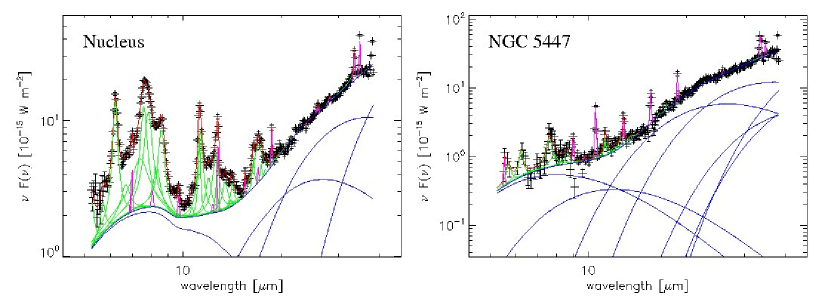
Figure 7.— The IRS spectra for the Nucleus and NGC 5447 are shown along with the PAHFIT results. The total PAHFIT spectrum is shown as well as the decomposition of the total (red) into dust continuum (blue), atomic emission lines (purple), and aromatic features (green). The silicate absorption has been applied to the PAHFIT results. No significant starlight is found by the PAHFIT program. The dust continuum is fit with up to 8 components with fixed temperatures and is meant to produce a continuum which is physical motivated (see section 4.13 of Smith et al., 2007b). This continuum fit is not unique and the strengths of the different components do not necessarily correspond to different real grain components.

There are a number of diagnostics of the physical conditions in the HII regions contained in the IRS spectra themselves as well as literature optical spectral studies. The IRS spectra give probes of the ionization ([NeIII]/[NeII], [SIV]/[SIII], [ArIII]/[ArII]) and electron density ([SIII] 18/[SIII] 33) (Giveon et al., 2002). The ionization probe is related to the radiation field hardness, but it is not easy to make a direct translation. The optical studies provide high quality metallicities [log(O/H)+12], electron temperatures, and ionization (e.g., [OIII] 5007/[OII] 3727). (Kennicutt et al., 2003a; Bresolin, 2006). Finally, the MIPS 24 µm flux provides a rough probe of the radiation field density convolved with the amount of dust present. Wu et al. (2006) used a similar measurement, $L_{22\micron}/V$, where $L_{22\micron}$ was determined from IRS Red Peakup images and $V$ is the volume of the region probed (in this case the whole galaxy). This was described as a probe of the UV radiation field density assuming dust absorbs most of the energy and there is a fairly constant conversion from $L_{22\micron}$ and total IR flux. In our case, the $V$ is similar for all our HII regions because we are probing regions in the same galaxy with photometry performed with the same sized apertures.

Figure 8.— Diagnostics of the physical conditions in HII regions are plotted versus each other to illustrate their interdependencies. These probes are the ionization ([NeIII]/[NeII] and [SIV]/[SIII] 18, dereddened [OIII] 5007/[OII] 3727), electron density ([SIII] 18/[SIII] 33), metallicity [log(O/H) + 12], the optical emission line electron temperature [T_e(O⁺,N⁺,S⁺)], and radiation field intensity (MIPS 24 µm flux).

The different diagnostics are not all independent and Fig. 8 illustrates this point. The correlations among the different ionization probes were seen in ISO observations of HII regions (Giveon et al., 2002) and starburst galaxies (Verma et al., 2003). Not surprisingly, we find the same for M101 HII regions for the correlation between [NeIII]/[NeII] and [SIV]/[SIII] 18 (Fig. 8a, [ArIII]/[ArII] is not plotted as both lines are only significantly detected in one of our HII regions). The infrared ([NeIII]/[NeII]) and optical (dereddened [OIII] 5007/[OII 3727]) probes of ionization are seen to be correlated (Fig. 8b), but not nearly as well as the two infrared ionization probes (Fig. 8a). Metallicity and ionization are known to be roughly correlated. This rough correlation is caused by decreasing line blanketing and harder spectra in hot stars as the metallicity decreases. In the M101 HII regions, we also see these two quantities are correlated (Fig. 8c), but the correlation has a larger scatter than can be accounted for by the observational uncertainties. Fig. 8d illustrates that all the HII regions have similar electron densities, $<100$ cm^-3, as determined from the [SIII] 18/[SIII] 33 line ratio (Giveon et al., 2002) as well as optical spectroscopy (Kennicutt et al., 2003a). This is likely due to the different ionization energies between [OII] (13.6 eV) and [NeII] (21.6 eV) and [SIII] (23.3 eV). The rough correlation between the optical and infrared ionization measures indicates that there may well be significant variation in the radiation field hardness among the different HII regions. The radiation field intensity as probed by the MIPS 24 µm flux is not correlated with any of the physical quantities (Fig. 8e) although this lack of correlation is mainly based on the large 24 µm flux seen for NGC 5461. Finally, the optically determined electron temperatures are well correlated with metallicity (Fig. 8f). Overall, there seem to be three quantities that probe different physical properties of the HII regions. They are log(O/H)+12 (metallicity and electron temperature), [NeIII]/[NeII] and [SIV]/[SIII] 18 (ionization), and MIPS 24 µm flux (radiation field intensity).

Given that the [NeIII]/[NeII] and [SIV]/[SIII] 18 ratios are well correlated, it is possible to combine the two ratios into a composite ionization measurement with smaller uncertainties. In this paper and Engelbracht et al. (2008), we propose a composite measure called the ionization index (or II for short). It is defined as the weighted average of log([SIV]/S[III] 18) converted to the [NeIII]/[NeII] scale and log([NeIII]/[NeII]). The conversion of [SIV]/S[III] 18 to the [NeIII]/[NeII] scale is done using the observed correlation for the M101 HII regions and the starburst galaxies presented by Engelbracht et al. (2008). This correlation for just the M101 HII regions (Fig. 8a) is

$$\log\left(y\right)=(0.93\pm 0.11)+(1.85\pm 0.34)\log\left(x\right)$$ (5)

where $x=$ [SIV]/[SIII] 18 and $y=$ [NeIII]/[NeII]. The combined correlation of the M101 HII regions and the starburst galaxies is

$$\log\left(y\right)=(0.71\pm 0.08)+(1.58\pm 0.13)\log\left(x\right).$$ (6)

We adopt the combined correlation to determine the II values for the M101 HII regions. Thus, II can be calculated from

$$\mathrm{II}=\log\left(\frac{\mathrm{[NeIII]}}{\mathrm{[NeII]}}\right)+\left[0.71+1.58\log\left(\frac{\mathrm{[SIV]}}{\mathrm{[SIII]18}}\right)\right].$$ (7)

We use the II values for the rest of this paper instead of the [NeIII]/[NeII] or [SIV]/[SIII] 18 ratios as the II has less noise and is available for all the M101 HII regions.

We have chosen to call the combined measurement of [NeIII]/[NeII] and [SIV]/[SIII] an ionization index as this is the physical measurement which is being made. Often these two ratios are used as an indicator of the radiation field hardness (or $T_{eff}$). These ratios are dependent on the metallicity, ionization parameter and morphology. and age of an HII region. The dependence is such that the ratios decrease as the metallicity increases, the ionization parameter decreases, and the age decreases (Rigby & Rieke, 2004). This explains why these ratios are only roughly correlated with metallicity. The scatter in the metallicity versus [NeIII]/[NeII] ratio (Fig. 8c) is likely due to different HII region ages and/or ionization parameters. Disentangling the different effects is complicated and beyond the scope of this paper as we are only interested in these ratios as a measure of the amount of processing which might have taken place in the HII regions.

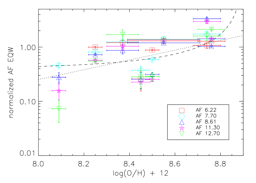
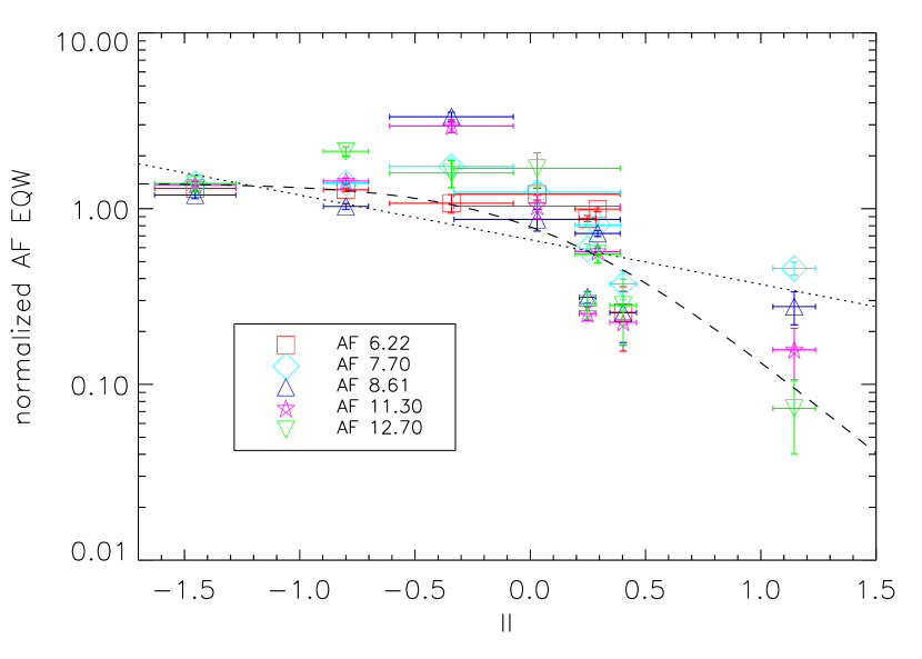
Figure 9.— The normalized equivalent widths of the 5 highest equivalent width aromatic features (AFs) are plotted versus metallicity (left) and ionization index (II [see §3.2)], right). The normalization was done to the average equivalent width of each AF. The normalization values are 0.87, 3.01, 1.04, 1.32, and 0.56 µm for the 6.22, 7.70, 8.61, 11.30, and 12.70 µm aromatic features, respectively. The dotted and dashed lines give the best fit power law and power law plus constant, respectively (see §3.2).

The equivalent widths of the aromatic features are plotted versus metallicity and II in Fig. 9. The equivalent width measures the strength of the aromatic features versus the underlying mid-infrared dust continuum emission. As both the aromatic features and underlying continuum are measured at the same wavelengths, they are likely to have undergone similar excitation and, therefore, the equivalent width is a measurement of the abundance ratio of the aromatic carriers to small dust grains. Visually, it appears that the equivalent width of the aromatic features is better correlated with II than with metallicity. We have quantified this by fitting the measurements with two different functions. The first is a simple power law

$$y=ax^{b}$$ (8)

where $x=10^{\mathrm{II}}$ and y is the normalized aromatic equivalent width. The second equation is a power law plus a constant with the form

$$y=\left[ax^{b}+c\right]^{-1}.$$ (9)

The best fits using both of these equations are shown in Fig. 9. The reduced $\chi^{2}$ values for the data versus metallicity are 356 and 339 for the simple power and power law plus a constant, respectively. The reduced $\chi^{2}$ values for the data versus II are 240 and 195 for the simple power and power law plus a constant, respectively. This indicates that the aromatic feature equivalent widths are better correlated with ionization than metallicity. In addition, the functional form favored is the power law plus constant (Eq. 9). The behavior of the aromatic equivalent widths can be described as constant up to a threshold II ($\sim 0$ which is a [NeIII]/[NeII] value of 1) and then a reduction in equivalent width with a power law form at higher II values. The best fit between the II and normalized equivalent width measurements is

$$y=\left[0.55x^{0.98}+0.73\right]^{-1}.$$ (10)

The expected values for the equivalent widths for a particular aromatic feature can be determined from this equation multiplied by the average equivalent widths that are given in the caption of Fig. 9.

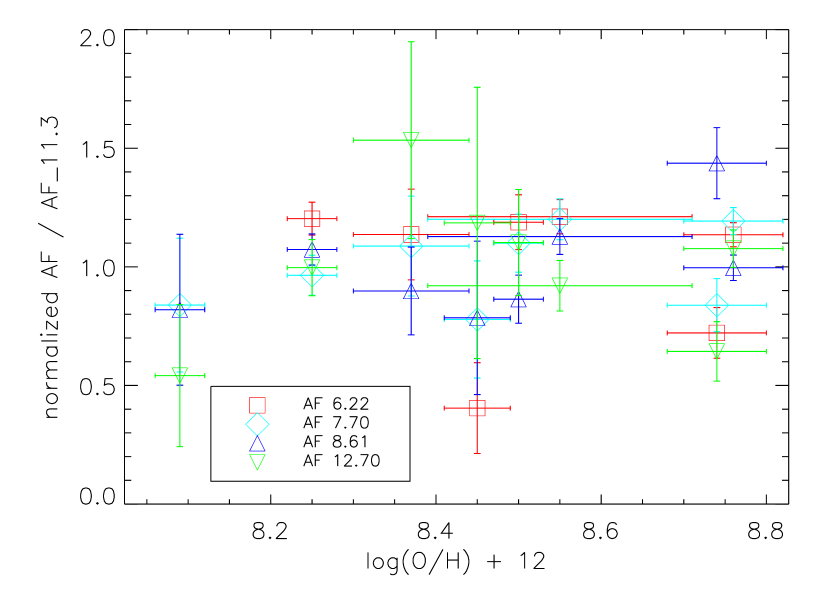
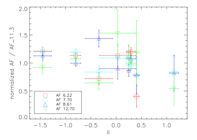
Figure 10.— The ratio of the strength of the 4 strongest aromatic features (AFs) to the 11.3 AF are plotted versus metallicity (left) and ionization index (II, right). The normalization was done to the average ratio of each AF. The normalization values are 1.01, 3.41, 0.80, and 0.57 for the 6.22, 7.70, 8.61, and 12.70 µm aromatic features, respectively.

The ratio of the integrated strengths of different aromatic features is a diagnostic of the physical mechanism of processing. For example, models using PAHs as the carriers of the aromatic features predict the strength of the 6.22, 7.70, and 8.61 µm features to strengthen relative to the 11.3 and 12.7 µm features as the ionization level increases or to weaken as the smaller PAHs are removed (Bakes et al., 2001; Peeters et al., 2002). In Fig. 10 we show the ratio of the 4 strongest aromatic features to the 11.3 µm feature versus metallicity and II. The ratios do not vary significantly from object to object nor does there seem to be a significant trend with either of the two diagnostics. While there is a large scatter in the ratios of around a factor of two, the large measurement uncertainties mean that the ratios could be consistent with no change with either of the two diagnostics. This is different than the preliminary result reported by Gordon et al. (2006a) where significant variation in the ratios was found. We have improved both the IRS data reductions and aromatic feature equivalent width measurements, which accounts for the differences. The lack of ratio variations is interesting in light of the strong weakening of the aromatics above a threshold in II (Fig. 9). The aromatic features weaken by over a factor of 10, but the ratio of different aromatics does not change by more than a factor of 2.

3.3. Photometric Measures of Aromatics

While IRS spectroscopy is clearly the most accurate way to study the aromatic features, it would be useful to be able to probe the aromatic feature strengths using some combination of IRAC and MIPS imaging. Having a photometric probe to the aromatic features would allow for a larger range of objects and environments to be studied given that imaging is faster to acquire and can probe regions that are too faint for spectroscopy. Engelbracht et al. (2005) proposed the combination of 8-to-4.5 and 8-to-24 µm flux density ratios as just such a measure of the aromatic feature strength given that the IRAC 8 µm band probes the strong 8 µm aromatic complex (composed of the 7.7, 8.3, and 8.6 µm aromatic features) and the IRAC 4.5 µm and MIPS 24 µm bands probe different parts of the small grain dust emission.

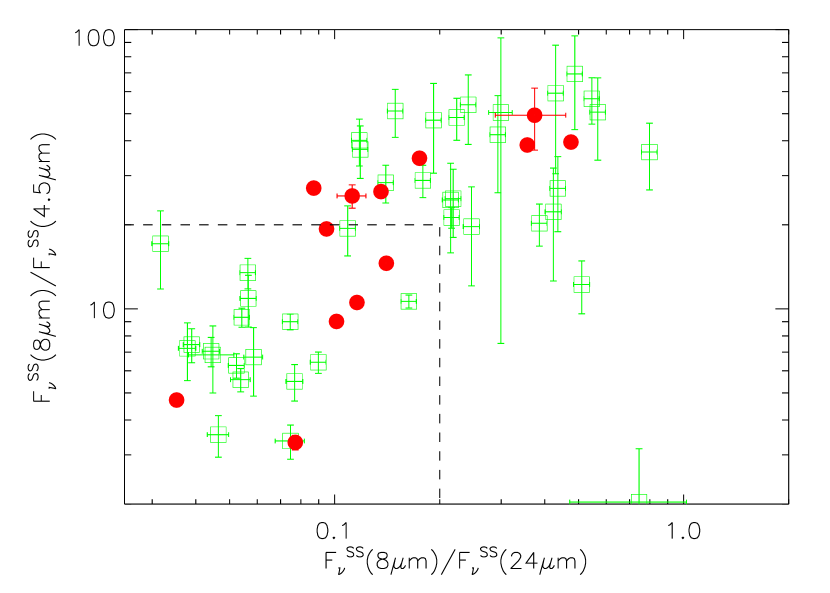
Figure 11.— The $f_{\nu}^{SS}(8~{}\micron)/f_{\nu}^{SS}(4.5~{}\micron)$ ratio is plotted versus the $f_{\nu}^{SS}(8~{}\micron)/f_{\nu}^{SS}(24~{}\micron)$ ratio where the superscript “SS” designates these fluxes as stellar subtracted. The contributions to the measured fluxes from stellar emission was subtracted by scaling the measured 3.6 µm flux by 0.57, 0.23, and 0.031 for the 4.5 µm, 8.0 µm, and 24 µm bands, respectively. The HII regions are plotted as solid, red circles and the starburst galaxies (Engelbracht et al., 2008) as open, green squares. The error bars are derived from the measurement uncertainties and include the contribution from stellar subtraction. The dotted line shows a spectroscopically-chosen color separation between galaxies with (outside the box) and without (inside the box) aromatic emission (Engelbracht et al., 2008).

The 8-to-4.5 and 8-to-24 µm flux density ratios are measuring something very similar to an aromatic feature equivalent width as it can be thought of as the ratio of the aromatic emission divided by the underlying small grain emission. It is not the same as an equivalent width as the small grain emission measurement is done at shorter and longer wavelengths (4.5 and 24 µm, respectively, instead of 8 µm) than is done when using the IRS spectroscopy. In other words, the 4.5 µm flux probes hotter and 24 µm cooler dust grains than the 8 µm spectroscopic continuum. Thus, variations in 8-to-4.5 and 8-to-24 µm can be due to changes in the dust emission continuum instead of the 8 µm aromatic complex. Yet if both ratios change in a consistent manner, it is highly likely it is the 8 µm aromatic complex which is varying. In Figure 11 we plot the 8-to-24 µm versus 8-to-4.5 µm flux density ratios for a sample of M101 HII regions and a sample of starburst galaxies Engelbracht et al. (2008). The M101 HII region photometry was performed on the MIPS 24 µm and IRAC 3.6, 4.5, & 8.0 images convolved to the 24 µm PSF (§2.3). The photometry was measured using a 10″ radius object aperture and a background annulus with radii from 13 to 20″and is given in Table 3. The IRAC 3.6 µm band is dominated by stellar emission and was used to subtract the stellar contribution from the longer wavelength measurements (Engelbracht et al., 2005). The starburst photometry is from Engelbracht et al. (2008) and was also corrected for stellar emission.

Table 3Photometry for M101 regions

name	IRAC1	IRAC2	IRAC3	IRAC4	MIPS24
	3.6 µm	4.5 µm	5.8 µm	8.0 µm	24 µm
	[mJy]	[mJy]	[mJy]	[mJy]	[mJy]
Nucleus	$15.00\pm 0.119$	$9.70\pm 0.083$	$19.20\pm 0.222$	$48.90\pm 0.675$	$96.20\pm 1.221$
Hodge 602	$3.09\pm 0.595$	$1.94\pm 0.364$	$3.78\pm 0.662$	$9.35\pm 1.545$	$23.20\pm 3.654$
Hodge 1013	$1.59\pm 0.051$	$1.47\pm 0.035$	$7.33\pm 0.166$	$20.00\pm 0.447$	$112.00\pm 0.531$
Searle 5	$1.17\pm 0.017$	$1.00\pm 0.012$	$4.82\pm 0.039$	$13.20\pm 0.126$	$36.20\pm 0.128$
NGC 5461	$7.01\pm 0.143$	$6.96\pm 0.121$	$28.40\pm 0.534$	$82.00\pm 1.392$	$923.00\pm 5.994$
NGC 5462	$1.37\pm 0.047$	$1.16\pm 0.040$	$4.08\pm 0.086$	$10.40\pm 0.213$	$74.50\pm 0.884$
NGC 5455	$1.92\pm 0.009$	$1.75\pm 0.009$	$5.36\pm 0.031$	$13.10\pm 0.082$	$134.00\pm 0.388$
NGC 5447	$1.75\pm 0.104$	$1.47\pm 0.091$	$4.62\pm 0.342$	$12.30\pm 0.898$	$106.00\pm 6.463$
Hodge 67	$0.19\pm 0.008$	$0.17\pm 0.006$	$0.43\pm 0.012$	$1.02\pm 0.026$	$6.94\pm 0.071$
Hodge 70/71	$0.26\pm 0.008$	$0.26\pm 0.006$	$0.52\pm 0.017$	$1.23\pm 0.043$	$10.20\pm 0.120$
Searle 12	$0.45\pm 0.007$	$0.44\pm 0.005$	$0.79\pm 0.009$	$1.76\pm 0.019$	$16.30\pm 0.079$
NGC 5471	$1.56\pm 0.012$	$1.80\pm 0.011$	$2.10\pm 0.019$	$4.66\pm 0.035$	$122.00\pm 0.777$
Hodge 681	$0.12\pm 0.008$	$0.10\pm 0.005$	$0.11\pm 0.005$	$0.14\pm 0.004$	$1.53\pm 0.042$

The plot shown in Fig. 11 is similar to Fig. 1 of Engelbracht et al. (2005) except that we have plotted the 8-to-4.5 µm instead of 4.5-to-8 µm flux ratio so that both the ratios plotted behave in a similar sense where larger ratios imply stronger aromatic features. In addition, we have subtracted the stellar contribution from all three bands involved using scaled 3.6 µm flux densities. These two ratios probe the behavior of the 8 µm aromatic complex plus underlying dust continuum emission versus shorter wavelength dust continuum emission (8.0/4.5) and longer wavelength dust continuum emission (8/24). Fig. 11 shows that the M101 HII regions and starburst galaxies show the same behavior and cover similar ranges in both ratios. This is not surprising given that the simplest model of a starburst is a collection of HII regions. However, it is important to confirm that HII regions have mid-IR SEDs similar to those of starburst galaxies and, as a result, are reasonable analogs for studying dust emission from starburst galaxies.

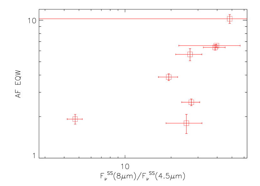
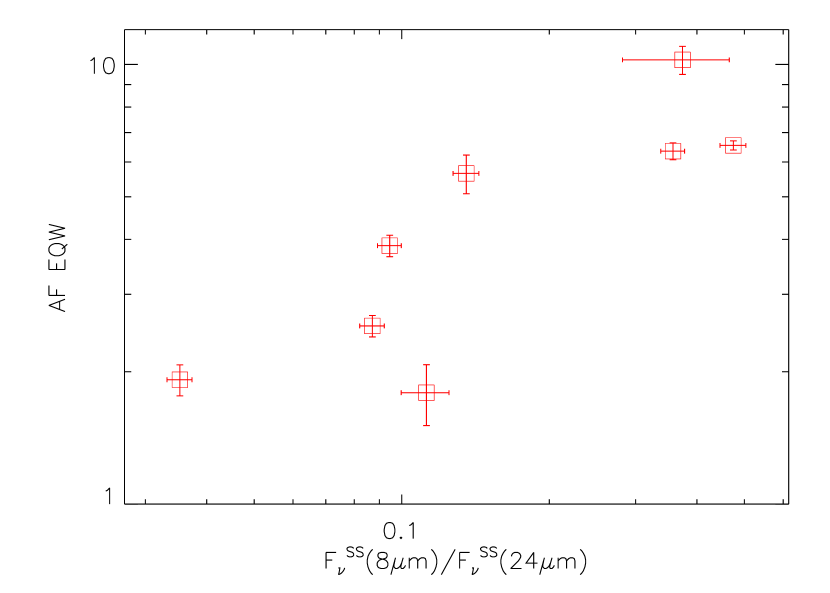
Figure 12.— The $F_{\nu}^{SS}(8~{}\micron)/F_{\nu}^{SS}(4.5~{}\micron)$ and $F_{\nu}^{SS}(8~{}\micron)/F_{\nu}^{SS}(24~{}\micron)$ ratios are shown plotted versus measured 8 µm aromatic feature complex equivalent width.

Given that we have spectroscopic and photometric measurements of the 8 µm aromatic feature complex, we can see how the photometric measure compares with the more accurate spectroscopic measurement. Figure 12 gives this comparison where the measured spectroscopic equivalent width of the 8 µm aromatic complex is plotted versus the 8-to-4.5 µm and 8-to-24 µm flux density ratios. It is clear that these two flux ratios are rough measures of the 8 µm complex. The 8-to-24 µm ratio is probably a better measure given that the relationship is more linear than that using the 8-to-4.5 µm ratio and the measurement uncertainties are smaller.

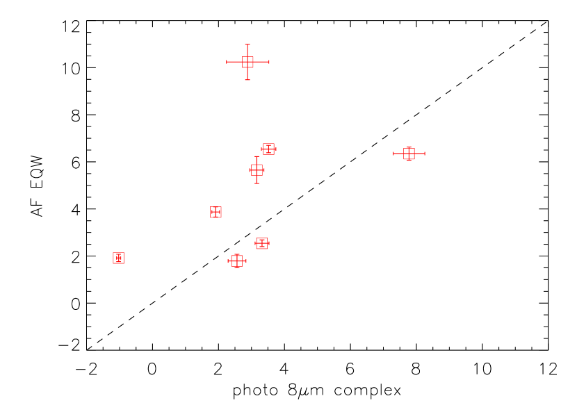
Figure 13.— The photometric (see §3.3) versus spectroscopic measurements of the 8 µm aromatic complex equivalent width are plotted. The dashed line shows the one-to-one relationship.

It is possible to combine both ratios in a way to create a better measure of the 8 µm complex. The basic idea is to use the 4.5 and 24 µm measurements to predict the continuum at 8 µm due to small grain emission and combine this continuum prediction with the measured 8 µm flux to create a photometric measure of the 8 µm equivalent width. Following Engelbracht et al. (2008), we find that it is best predicted using

$$F_{\nu}(8\micron)_{\mathrm{cont}}=F_{\nu}(4.5\micron)^{0.66}\times F_{\nu}(24\micron)^{0.34}$$ (11)

which results from assuming the small grain emission follows a power law. Unlike Engelbracht et al. (2008), we have not used the stellar subtracted fluxes to determine $F_{\nu}(8~{}\micron)_{\mathrm{cont}}$ as we do not have K band fluxes to help measure the stellar flux and the stellar contribution is expected to be small for these resolved HII regions. Using the stellar subtracted fluxes produces systematically larger photometric than the measured spectroscopic equivalent widths. The photometric equivalent width is then

$$\mathrm{EQW}(8~{}\micron)_{\mathrm{photo}}=\left(\frac{F_{\nu}(8\micron)}{F_{\nu}(8\micron)_{\mathrm{cont}}}-1\right)\Delta\lambda.$$ (12)

where $\delta\lambda=2.69$ µm and is the width of the IRAC 8 µm band. This assumes that the 8 µm complex fills the IRAC 8 µm band which is the case for many of the HII regions, but not all of them (see Fig. 3). We have computed the photometry equivalent widths for the M101 regions and plotted them versus the spectroscopic equivalent widths in Fig. 13. The photometric equivalent width measurement produces a good rough measurement of the 8 µm aromatic complex for the M101 regions. A similar result is found by Engelbracht et al. (2008) for the starburst galaxy sample.

3.4. Morphology of Aromatic Emission

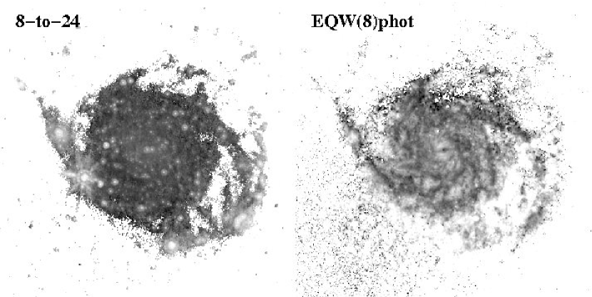
Figure 14.— The 8-to-24 and $\mathrm{EQW}(8~{}\micron)_{\mathrm{photo}}$ images of M101 are shown. The images are displayed in reverse B/W using a asinh stretch with ranges from 0.1–2.0 and 3–30 and pivots of 0.5 and 5.0, respectively. The inner 20$\arcmin$ of M101 is shown. Only pixels with measurements above the sky noise are displayed. The $\mathrm{EQW}(8~{}\micron)_{\mathrm{photo}}$ image shows significant noise due to instrumental signatures present in the IRAC 8 µm mosaic (see Fig. 1).

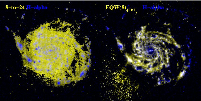
Figure 15.— The 8-to-24 and $\mathrm{EQW}(8~{}\micron)_{\mathrm{photo}}$ images of M101 are shown in yellow along with the H$\alpha$ image in blue. The inner 20$\arcmin$ of M101 is shown. Only pixels with measurements above the sky noise are displayed.

The IRAC and MIPS images of M101 can be used to probe the morphology of M101 in the 8 µm aromatic complex by applying the photometric measurement techniques introduced in §3.3. Fig. 14 shows the simple 8-to-24 µm flux density ratio image and the $\mathrm{EQW}(8~{}\micron)_{\mathrm{photo}}$ image. The IRAC images were convolved to the 24 µm resolution (§2.3) of 6$\arcsec$ (0.2 kpc at 6.7 Mpc) before computing either composite image. Caution should be exercised in interpreting these images as both involve stellar subtracted images. The stellar subtraction is done using a multiplicative scaling of the IRAC 3.6 µm image and the accuracy of this method has only been shown for integrated fluxes. This method will oversubtract regions where the emission in the 3.6 µm image is dominated by dust emission instead of stellar emission. While the $\mathrm{EQW}(8~{}\micron)_{\mathrm{photo}}$ image is expected to be a more accurate estimate of the true 8 µm aromatic complex equivalent width than the 8-to-24 µm image, it suffers from higher noise given the sensitivity of this measurement to the more uncertain stellar subtracted 4.5 µm flux and 8 µm instrumental residuals. Both images show that the aromatic features are depressed in HII regions (white regions in Fig. 1). This is illustrated in Fig. 15 where the H$\alpha$ image is shown in blue and the 8-to-24 µm and $\mathrm{EQW}(8~{}\micron)_{\mathrm{photo}}$ images are shown in yellow. The preponderance of yellow and blue in the first image shows that the 8-to-24 µm is anti-correlated with H$\alpha$ emission. This is an indication that the 8 µm flux is depressed and/or the 24 µm flux is enhanced in HII regions. The $\mathrm{EQW}(8~{}\micron)_{\mathrm{photo}}$+H$\alpha$ image directly probes the strength of the 8 µm aromatic complex versus H$\alpha$ and shows that the separation between the yellow and blue is not as clean as in the 8-to-24 µm+H$\alpha$ image. Thus, the enhancement of 24 µm emission in HII regions is a significant contributer to the morphology of the 8-to-24 µm image. In other words, the dust in HII regions is hotter (emitting more at 24 µm) than the surrounding dust, but this hotter dust does not have a corresponding increase in the 8 µm continuum or aromatic emission to keep the 8-to-24 µm ratio constant. But there is clearly also a change in the 8 µm emission, given that there are large HII complexes (e.g., NGC 5462, NGC 5447) in the second image which show the expected morphology with aromatic emission (yellow) surrounding the H$\alpha$ emission.

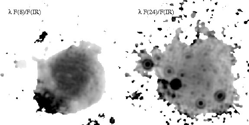
Figure 16.— The images of M101 in $\lambda F(8~{}\micron)/F(IR)$ and $\lambda F(24~{}\micron)/F(IR)$ are shown. The images are displayed in reverse B/W with a linear stretch from 0–0.30 and 0–15, respectively. This same region displayed in Fig. 2 is shown (30$\arcmin$ roughly centered on M101).

Finally, the aromatic feature and underlying continuum emission can be compared to that of the large grains by including the longer wavelength MIPS images in the analysis. Fig. 16 shows two images: the first is the ratio of the 8 µm flux to the total infrared ($\lambda F(8~{}\micron)/F(IR)$) and the second is the ratio of the 24 µm flux to the total infrared ($\lambda F(24~{}\micron)/F(IR)$). Generally, the 8 µm emission traces the aromatic features (with a minor contribution from the continuum), the 24 µm emission traces the hot dust emission from small grains, and the total infrared traces the bulk of the dust grains which dominate the dust mass and have a peak emission around 160 µm (see Fig. 6). To first order, $\lambda F(8~{}\micron)/F(IR)$ and $\lambda F(24~{}\micron)/F(IR)$ trace the ratio of aromatic grain mass to dust mass and small grain mass to dust mass, respectively, modified by the illuminating radiation field. All the images used were first convolved to the 160 µm resolution of 40″ (1.3 kpc at 6.7 Mpc) using the kernels described in §2.3. The total infrared flux was calculated by a simple integration of the IRAC 8 µm through MIPS 160 µm images. The $\lambda F(8~{}\micron)/F(IR)$ image is dominated by a high ratio in the inner region with a fairly abrupt drop to much lower values. The brightest HII regions are seen to have shallow depressions compared to other regions at the same radii. The $\lambda F(24~{}\micron)/F(IR)$ image displays a different morphology with a relatively flat ratio overall with strong enhancements in the HII regions. The depression of the aromatic emission is not due to lack of exciting photons as these are clearly present given the enhancement of the 24 µm emission. The depression of the aromatic emission in HII regions must then be due to processing of the carriers of these features. The behavior of these two ratios supports the results of the comparison to the H$\alpha$ given in the previous paragraph. The variations of the 8 µm emission are dominated by variations in ionization while the 24 µm emissions are dominated by the radiation field intensity (as traced by the H$\alpha$ emission).

4. Discussion

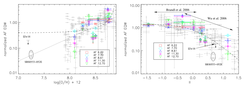
Figure 17.— The normalized equivalent widths of the 5 highest equivalent width aromatic features (AFs) are plotted versus metallicity (left) and ionization index (II, right). These two plots are the same as shown in Fig. 9 but now include the starburst sample from Engelbracht et al. (2008) in grey. The locations of the two most metal poor galaxies (SBS0335-052E and IZw18) are labeled. In addition, the II ranges probed in Brandl et al. (2006) and Wu et al. (2006) are indicated. The normalization was done the same as in Fig. 9.

The behavior of the aromatic feature equivalent widths versus metallicity and II seen in this paper for M101 HII regions is also seen for starburst galaxies. This is shown in Fig. 17 which combines the measurements for the M101 HII regions presented in this paper with the starburst galaxy measurements from Engelbracht et al. (2008). Both samples show a better correlation of the aromatic equivalent widths versus II than metallicity. The combined M101 HII region and starburst galaxy samples probe ionization indexes between -1.5 and 1.4 (equivalent to [NeIII]/[NeII] ratios of 0.03–25) and metallicities (log(O/H)+12) from 7.9–8.8. There are two galaxies (SBS0335-052E and IZw18) which have metallicities below 7.9, but this is not enough points to statistically probe the behavior in this range. It is interesting to note that these two galaxies do not have the most extreme II values and fit fairly well in the trend of II versus aromatic feature equivalent widths. The residuals of fit of II versus aromatic feature equivalent width were plotted versus metallicity to see if the scatter around the fit was due to metallicity, but no trend was present.

The correlation of the aromatic equivalent widths with II is not a simple power law, but shows a change at around a II value of zero. Below this value, the equivalent widths are fairly constant indicating that the material responsible for the aromatic features is as robust as the material responsible for the underlying dust continuum emission. Above this value, the equivalent widths drop significantly with increasing II. This implies that the material responsible for the aromatic features is being modified/destroyed at a faster rate than the material responsible for the underlying dust continuum emission.

The complex behavior of the aromatic equivalent widths with II explains the seemingly contradictory results found by previous authors. Brandl et al. (2006) studied low ionizations ($-1.25<\mbox{II}<0.05$) and found no variation. Wu et al. (2006) studied high ionizations ($-0.3<\mbox{II}<1.3$) and found large variations. Only by studying the full range of II values does the complex nature of the correlation between II and aromatic equivalent width emerge.

The complex behavior of the aromatic equivalent widths also explains why the bright point sources (e.g., HII regions) in M101 change fairly abruptly from yellow to red at approximately the same radii in Fig. 2. The colors of the HII regions are primarily composed of green (IRAC 8 µm) and red (MIPS 24 µm). In the inner regions of M101, the HII regions have high metallicity and low ionization (e.g., Fig. 8c). This means that they have II values below 0 and, thus, normal aromatic equivalent widths (e.g., IRAC 8 µm emission). In the outer regions, the HII regions have low metallicity and high ionization. Thus, they have much weaker aromatic emission which strongly reduces the green color. Red color in this particular type of 3 color image is a strong indication of weak aromatic emission.

Our finding that the aromatic equivalent widths in the M101 HII regions and starburst galaxies correlates better with a measure of processing (ionization) than with a measure of formation (metallicity) is not too surprising. There has been ample evidence for such processing in spatially resolved studies in reflection nebulae and HII regions in the Milky Way (Cesarsky et al., 2000; Berné et al., 2007). But until this work, it is not been clear if the spatially resolved processing of the aromatic carriers also applies to the global spectra of massive star forming regions (i.e., HII regions and starburst galaxies). This work indicates that the processing of the aromatic carriers is happening on a global scale in massive star forming regions.

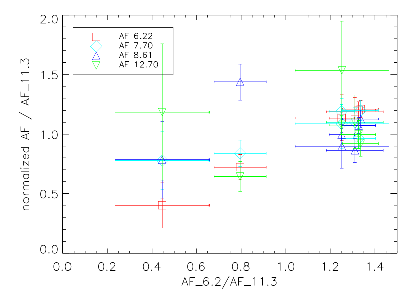
Figure 18.— The ratio of the strength of the 4 strongest aromatic features (AFs) to the 11.3 AF are plotted versus the 6.2/11.3 AFs. The normalization was done to the average ratio of each AF. The normalization values are 1.01, 3.41, 0.80, and 0.57 for the 6.22, 7.70, 8.61, and 12.70 µm aromatic features, respectively. The points for the 6.22 AF defined the one-to-one correspondence.

Models where PAH molecules are the carriers of the aromatic features would predict a correlation of the ratios of different aromatic features with ionization index if the processing mechanisms were ionization or size selective destruction. The lack of such a correlation (see Fig. 10) seems to imply that these two processing mechanisms may not be the dominant cause of the strong correlation seen with ionization index. Fig. 18 plots the ratio of the strongest 4 aromatic features and the 11.3 µm aromatic versus the 6.2/11.3 aromatic ratio. In PAH models of the aromatic features (Galliano, 2006), the 6.2 µm aromatic traces small, ionized PAHs and the 11.3 µm aromatic traces larger, neutral PAHs. Thus, the 6.2/11.3 ratio traces ionized/neutral and/or small/large PAHs. The 7.70 µm and 8.61 µm aromatics also trace small, ionized PAHs and the 12.7 µm larger, neutral PAHs. While there is scatter in Fig. 18, the 7.70/11.3 and 8.61/11.3 ratios correlate fairly well with the 6.2/11.3 ratio. On the other hand, the 12.7/11.3 does not correlate at all with the 6.2/11.2 ratio. Thus, the behavior of the relative strengths of the 5 strongest aromatic features is consistent with the PAH molecule model. The lack of correlation seen between the variations in the aromatic features with ionization (Fig. 10) is not consistent with the PAH molecule model.

There seem to be two different effects at work in HII regions. The first is consistent with the PAH molecule model and explains the behavior of the spatially resolved aromatic feature ratios. The second is required to explain the good correlation between the decrease in the globally integrated aromatic equivalent widths and increasing ionization and the lack of a correlation between the aromatic feature ratios and ionization index. This second effect may be related to the small grain model for the aromatic features. If small grains can produce aromatic features and provide the parent population of the PAH molecules in photodissociation regions regions (PDRs) (Berné et al., 2007) then it may be that the decrease in the strength of the aromatic equivalent width is due to processing of the small grains. Another possible explanation could be that the sizes of the PDRs in regions with harder radiation fields (and, thus, higher ionizations) are significantly reduced. As the aromatic features are known to emerge predominately from the PDR regions surrounding the HII regions and the underlying continuum emission emerges from the whole HII region, decreasing the area of the PDR would result in smaller aromatic equivalent widths. Decreasing PDR areas with lower metallicities may also explain the low CO emission seen in low metallicity starburst galaxies (Leroy et al., 2007).

The processing of the aromatic feature carriers by massive star formation is one line of evidence that such star formation actively modifies the properties of the surrounding dust grains. There is additional evidence that active, high-mass star formation modifies the properties of nearby dust grains. One observational signature of this effect is the lack of the 2175 Å extinction bump in starburst galaxies (Calzetti et al., 1994; Gordon et al., 1997). Ultraviolet (UV) extinction curves studies in the Small Magellanic Cloud (Gordon & Clayton, 1998), Large Magellanic Cloud (Misselt et al., 1999), and Milky Way (Clayton et al., 2000; Valencic et al., 2003) paint a consistent picture where the 2175 Å bump is depressed and the overall UV extinction increased in regions near massive star formation (Gordon et al., 2003). These changes in the UV extinction can be explained by the removal of the small graphite grains that produce the 2175 Å feature, along with an increase in the number of small silicate grains that are responsible for the majority of the ultraviolet extinction (Weingartner & Draine, 2001; Clayton et al., 2003). Given that these changes are in the small grain populations of the dust, it is not surprising that similar changes are seen in the mid-infrared where the small grains emit their absorbed energy. It is not clear if the changes seen in the aromatic features are directly correlated with the changes seen in the 2175 Å feature. More work in both the ultraviolet and mid-infrared is needed to answer this question.

5. Summary and Conclusions

We have studied trends in aromatic feature behavior with metallicity (log(O/H)+12 = 7.9–8.8) and ionization (II = -1.5–1.4 or [NeIII]/[NeII] = 0.03–25). Over this range, we have found that the equivalent width of the aromatic features is better correlated with the ionization index (II) than metallicity (log(O/H)+12) in both the M101 regions studied in this paper as well as the starburst galaxies presented in Engelbracht et al. (2008). The data available for metallicities between log(O/H)+12 = 7.1–7.9 are not sufficient to probe these trends for such low metallicities. Our result implies that the decrease in aromatic equivalent widths seen in regions of massive star formation (e.g., HII regions and starburst galaxies) is primarily due to processing, not formation. This is not to say that formation does not play a role, but just that it is not the dominant effect. The finding of processing of the aromatic carriers is consistent with existing evidence that the 2175 Å extinction feature carrier is processed in regions of massive star formation.

We found that the correlation of the aromatic equivalent widths with II is not a single power law as has been proposed in previous works. Instead the aromatic equivalent widths are constant till a threshold II of $\sim$0 and then decrease. This decrease is well fit with a power law. This more complex behavior is consistent with previous work (Brandl et al., 2006) and (Wu et al., 2006) which probed a narrower range of II and seemed to find conflicting results. Only the large range in both II and metallicity probed in this work and the companion work of Engelbracht et al. (2008) allowed for the true nature of the aromatic feature variations to be revealed.

The lack of a clear dependence of the ratio of different aromatic features to the 11.3 aromatic feature on II calls into question either ionization or size selective destruction of PAH molecules as the mechanism for the observed reduction in the aromatic equivalent width versus ionization. This might indicate a more solid material origin for the aromatics (Berné et al., 2007) which dominate the global measurements of HII regions. Or it might imply that the area of the PDR regions decreases with respect to the area of the small grain emission as the radiation field hardness (and thus ionization) increases.

Table 4Atomic Emission Line Strengths

name	[ArII]	[ArIII]	[SIV]	[NeII]	[NeIII]	[SIII] 18	[SIII] 33	[SiII]
	7.0 µm	9.0 µm	10.5 µm	12.8 µm	15.5 µm	18.7 µm	33.5 µm	34.8 µm
Nucleus	$3.30\pm 0.51$	$\cdots$	$\cdots$	$7.57\pm 0.51$	$1.20\pm 0.25$	$4.50\pm 0.51$	$18.78\pm 0.89$	$20.26\pm 0.79$
Hodge 602	$1.00\pm 0.23$	$\cdots$	$0.34\pm 0.12$	$2.30\pm 0.16$	$\cdots$	$1.54\pm 0.13$	$3.74\pm 0.12$	$3.48\pm 0.14$
Searle 5	$1.04\pm 0.17$	$0.09\pm 0.09$	$0.18\pm 0.05$	$4.13\pm 0.16$	$0.16\pm 0.11$	$4.01\pm 0.18$	$20.36\pm 0.28$	$9.14\pm 0.18$
NGC 5461	$1.78\pm 5.33$	$10.74\pm 0.81$	$28.39\pm 0.81$	$27.32\pm 1.54$	$56.09\pm 5.82$	$60.56\pm 3.94$	$259.21\pm 5.53$	$80.58\pm 3.67$
NGC 5462	$0.86\pm 0.53$	$2.25\pm 0.50$	$2.75\pm 1.21$	$4.34\pm 7.83$	$6.50\pm 1.95$	$7.46\pm 1.49$	$43.90\pm 1.02$	$15.01\pm 0.70$
NGC 5455	$0.34\pm 1.61$	$1.25\pm 0.09$	$3.08\pm 0.09$	$3.85\pm 0.15$	$11.19\pm 3.19$	$7.93\pm 1.68$	$46.14\pm 0.74$	$18.63\pm 0.59$
NGC 5447	$0.25\pm 0.11$	$0.92\pm 0.11$	$3.33\pm 0.10$	$1.61\pm 0.20$	$4.27\pm 0.56$	$5.41\pm 0.64$	$27.51\pm 1.31$	$10.60\pm 1.07$
NGC 5471	$\cdots$	$0.52\pm 0.15$	$12.92\pm 0.73$	$0.96\pm 0.29$	$20.63\pm 2.33$	$8.47\pm 1.38$	$32.60\pm 0.75$	$11.27\pm 0.57$

Table 5Aromatic Emission Line Strengths

name	5.7 µm	6.2 µm	7.7 µm	8.3 µm	8.6 µm	10.7 µm	11.3 µm	12.0 µm	12.7 µm	14.0 µm	17.0 µm
Nucleus	$7.86\pm 1.87$	$77.06\pm 1.78$	$271.43\pm 7.87$	$23.36\pm 2.00$	$56.62\pm 2.14$	$1.64\pm 0.47$	$61.58\pm 2.36$	$15.98\pm 1.07$	$36.27\pm 2.27$	$1.04\pm 0.57$	$55.12\pm 3.72$
Hodge 602	$2.53\pm 1.25$	$9.61\pm 1.16$	$37.42\pm 3.83$	$1.76\pm 0.90$	$16.03\pm 0.95$	$1.37\pm 0.24$	$12.08\pm 1.03$	$1.63\pm 0.38$	$4.25\pm 0.74$	$\cdots$	$4.97\pm 0.42$
Searle 5	$\cdots$	$12.54\pm 0.44$	$41.64\pm 2.20$	$1.03\pm 0.49$	$9.77\pm 0.45$	$0.02\pm 0.13$	$9.39\pm 0.45$	$1.88\pm 0.22$	$4.73\pm 0.50$	$0.59\pm 0.14$	$1.99\pm 0.30$
NGC 5461	$6.64\pm 1.25$	$66.21\pm 2.58$	$205.47\pm 13.74$	$12.74\pm 3.50$	$40.30\pm 3.08$	$2.48\pm 1.01$	$50.56\pm 4.50$	$14.73\pm 2.41$	$30.49\pm 5.56$	$\cdots$	$3.21\pm 4.16$
NGC 5462	$1.46\pm 1.14$	$20.21\pm 1.54$	$64.84\pm 7.92$	$4.42\pm 1.86$	$13.38\pm 1.89$	$1.34\pm 0.64$	$16.13\pm 2.42$	$1.88\pm 1.30$	$13.54\pm 3.05$	$2.95\pm 0.71$	$0.72\pm 1.18$
NGC 5455	$0.78\pm 0.64$	$14.42\pm 0.48$	$38.75\pm 2.86$	$2.84\pm 0.49$	$10.77\pm 0.42$	$0.39\pm 0.16$	$10.87\pm 0.51$	$2.34\pm 0.32$	$5.93\pm 0.65$	$0.63\pm 0.21$	$\cdots$
NGC 5447	$0.50\pm 0.44$	$1.30\pm 0.52$	$8.41\pm 1.58$	$1.35\pm 0.74$	$2.12\pm 0.68$	$\cdots$	$2.93\pm 0.75$	$0.54\pm 0.37$	$1.90\pm 0.78$	$\cdots$	$2.67\pm 1.24$
NGC 5471	$0.24\pm 0.69$	$\cdots$	$8.82\pm 0.76$	$\cdots$	$2.15\pm 0.46$	$1.27\pm 0.29$	$2.85\pm 0.92$	$\cdots$	$0.84\pm 0.38$	$0.74\pm 0.49$	$0.58\pm 1.73$

Table 6Aromatic Emission Line Equivalent Widths

name	5.7 µm	6.2 µm	7.7 µm	8.3 µm	8.6 µm	10.7 µm	11.3 µm	12.0 µm	12.7 µm	14.0 µm	17.0 µm
Nucleus	$0.16\pm 0.04$	$1.44\pm 0.03$	$4.91\pm 0.14$	$0.46\pm 0.04$	$1.17\pm 0.04$	$0.05\pm 0.01$	$1.90\pm 0.07$	$0.51\pm 0.03$	$1.18\pm 0.07$	$0.03\pm 0.02$	$1.46\pm 0.10$
Hodge 602	$0.29\pm 0.14$	$1.21\pm 0.15$	$6.09\pm 0.62$	$0.35\pm 0.18$	$3.80\pm 0.23$	$0.54\pm 0.09$	$3.92\pm 0.34$	$0.41\pm 0.10$	$0.89\pm 0.16$	$\cdots$	$0.59\pm 0.05$
Searle 5	$\cdots$	$1.47\pm 0.05$	$4.85\pm 0.26$	$0.13\pm 0.06$	$1.36\pm 0.06$	$0.00\pm 0.03$	$1.81\pm 0.09$	$0.33\pm 0.04$	$0.78\pm 0.08$	$0.08\pm 0.02$	$0.17\pm 0.03$
NGC 5461	$0.13\pm 0.02$	$0.99\pm 0.04$	$2.07\pm 0.14$	$0.12\pm 0.03$	$0.36\pm 0.03$	$0.02\pm 0.01$	$0.34\pm 0.03$	$0.09\pm 0.01$	$0.16\pm 0.03$	$\cdots$	$0.01\pm 0.01$
NGC 5462	$0.11\pm 0.08$	$1.36\pm 0.10$	$4.35\pm 0.53$	$0.32\pm 0.13$	$0.99\pm 0.14$	$0.12\pm 0.06$	$1.37\pm 0.21$	$0.15\pm 0.10$	$0.95\pm 0.21$	$0.15\pm 0.04$	$0.02\pm 0.03$
NGC 5455	$0.07\pm 0.06$	$1.12\pm 0.04$	$2.83\pm 0.21$	$0.21\pm 0.04$	$0.82\pm 0.03$	$0.03\pm 0.01$	$0.75\pm 0.04$	$0.14\pm 0.02$	$0.31\pm 0.03$	$0.02\pm 0.01$	$\cdots$
NGC 5447	$0.14\pm 0.12$	$0.29\pm 0.12$	$1.31\pm 0.25$	$0.19\pm 0.11$	$0.29\pm 0.09$	$\cdots$	$0.30\pm 0.08$	$0.05\pm 0.03$	$0.16\pm 0.06$	$\cdots$	$0.10\pm 0.04$
NGC 5471	$0.08\pm 0.22$	$\cdots$	$1.60\pm 0.14$	$\cdots$	$0.32\pm 0.07$	$0.11\pm 0.03$	$0.21\pm 0.07$	$\cdots$	$0.04\pm 0.02$	$0.03\pm 0.02$	$0.01\pm 0.03$

References

- Allamandola et al. (1985) Allamandola, L. J., Tielens, A. G. G. M., & Barker, J. R. 1985, ApJ, 290, L25
- Alonso-Herrero et al. (2006) Alonso-Herrero, A., et al. 2006, ApJ, 650, 835
- Bakes et al. (2001) Bakes, E. L. O., Tielens, A. G. G. M., & Bauschlicher, C. W. 2001, ApJ, 556, 501
- Berné et al. (2007) Berné, O., et al. 2007, A&A, 469, 575
- Bosma et al. (1981) Bosma, A., Goss, W. M., & Allen, R. J. 1981, A&A, 93, 106
- Brandl et al. (2006) Brandl, B. R., et al. 2006, ApJ, 653, 1129
- Bresolin (2006) Bresolin, F. 2006, ArXiv Astrophysics e-prints
- Brigham (1988) Brigham, E. O. 1988, The fast Fourier transform and its applications. (Englewood Cliffs, N.J.: Prentice-Hall, 1988)
- Calzetti et al. (2007) Calzetti, D., et al. 2007, ApJ, 666, 870
- Calzetti et al. (1994) Calzetti, D., Kinney, A. L., & Storchi-Bergmann, T. 1994, ApJ, 429, 582
- Cesarsky et al. (2000) Cesarsky, D., et al. 2000, A&A, 354, L87
- Clayton et al. (2000) Clayton, G. C., Gordon, K. D., & Wolff, M. J. 2000, ApJS, 129, 147
- Clayton et al. (2003) Clayton, G. C., et al. 2003, ApJ, 588, 871
- Cohen et al. (2001) Cohen, M., et al. 2001, AJ, 121, 1180
- Dale et al. (2005) Dale, D. A., et al. 2005, ApJ, 633, 857
- Dale et al. (2007) —. 2007, ApJ, 655, 863
- Dale & Helou (2002) Dale, D. A. & Helou, G. 2002, ApJ, 576, 159
- Devereux & Young (1990) Devereux, N. A. & Young, J. S. 1990, ApJ, 359, 42
- Draine et al. (2007) Draine, B. T., et al. 2007, ApJ, 663, 866
- Duley & Williams (1983) Duley, W. W. & Williams, D. A. 1983, MNRAS, 205, 67P
- Engelbracht et al. (2007) Engelbracht, C. W., et al. 2007, PASP, 119, 994
- Engelbracht et al. (2006) Engelbracht, C. W., et al. in , Astronomical Society of the Pacific Conference Series, Vol. 357, Astronomical Society of the Pacific Conference Series, ed. L. ArmusW. T. Reach, 215
- Engelbracht et al. (2005) —. 2005, ApJ, 628, L29
- Engelbracht et al. (2008) —. 2008, ApJ, in press
- Fazio et al. (2004) Fazio, G. G., et al. 2004, ApJS, 154, 10
- Freedman et al. (2001) Freedman, W. L., et al. 2001, ApJ, 553, 47
- Galliano (2006) Galliano, F. 2006, ArXiv Astrophysics e-prints
- Galliano et al. (2005) Galliano, F., et al. 2005, A&A, 434, 867
- Gillett et al. (1973) Gillett, F. C., Forrest, W. J., & Merrill, K. M. 1973, ApJ, 183, 87
- Giveon et al. (2002) Giveon, U., et al. 2002, ApJ, 566, 880
- Gordon et al. (1997) Gordon, K. D., Calzetti, D., & Witt, A. N. 1997, ApJ, 487, 625
- Gordon & Clayton (1998) Gordon, K. D. & Clayton, G. C. 1998, ApJ, 500, 816
- Gordon et al. (2003) Gordon, K. D., et al. 2003, ApJ, 594, 279
- Gordon et al. (2007) —. 2007, PASP, 119, 1019
- Gordon et al. (2006a) —. 2006a, ASP Conf. Ser., in press
- Gordon et al. (2006b) Gordon, K. D., et al. in , Astronomical Society of the Pacific Conference Series, Vol. 357, Astronomical Society of the Pacific Conference Series, ed. L. ArmusW. T. Reach, 188
- Gordon et al. (2005) —. 2005, PASP, 117, 503
- Hippelein et al. (1996) Hippelein, H., et al. 1996, A&A, 315, L82
- Houck et al. (2004a) Houck, J. R., et al. 2004a, ApJS, 154, 211
- Houck et al. (2004b) —. 2004b, ApJS, 154, 18
- Jarrett et al. (2003) Jarrett, T. H., et al. 2003, AJ, 125, 525
- Jones & d’Hendecourt (2000) Jones, A. P. & d’Hendecourt, L. 2000, A&A, 355, 1191
- Kennicutt et al. (2003a) Kennicutt, R. C., Bresolin, F., & Garnett, D. R. 2003a, ApJ, 591, 801
- Kennicutt et al. (2003b) Kennicutt, Jr., R. C., et al. 2003b, PASP, 115, 928
- Kraemer et al. (2002) Kraemer, K. E., et al. 2002, AJ, 124, 2990
- Lemke et al. (1996) Lemke, D., et al. 1996, A&A, 315, L64
- Leroy et al. (2007) Leroy, A., et al. 2007, ApJ, 663, 990
- Li & Draine (2001) Li, A. & Draine, B. T. 2001, ApJ, 554, 778
- Lu et al. (2003) Lu, N., et al. 2003, ApJ, 588, 199
- Lutz et al. (1998) Lutz, D., et al. 1998, ApJ, 505, L103
- Madden et al. (2006) Madden, S. C., et al. 2006, A&A, 446, 877
- Marleau et al. (2006) Marleau, F. R., et al. 2006, ApJ, 646, 929
- Misselt et al. (1999) Misselt, K. A., Clayton, G. C., & Gordon, K. D. 1999, ApJ, 515, 128
- Moustakas & Kennicutt (2006) Moustakas, J. & Kennicutt, Jr., R. C. 2006, ApJ, 651, 155
- Odenwald et al. (1998) Odenwald, S., Newmark, J., & Smoot, G. 1998, ApJ, 500, 554
- Papoular et al. (1989) Papoular, R., et al. 1989, A&A, 217, 204
- Peeters et al. (2004) Peeters, E., et al. Astronomical Society of the Pacific Conference Series, Vol. 309, , Astrophysics of Dust, ed. A. N. WittG. C. Clayton & B. T. Draine, 141–+
- Peeters et al. (2002) Peeters, E., et al. 2002, A&A, 390, 1089
- Popescu et al. (2005) Popescu, C. C., et al. 2005, ApJ, 619, L75
- Reach et al. (2005) Reach, W. T., et al. 2005, PASP, 117, 978
- Rice et al. (1988) Rice, W., et al. 1988, ApJS, 68, 91
- Rieke et al. (2004) Rieke, G. H., et al. 2004, ApJS, 154, 25
- Rigby & Rieke (2004) Rigby, J. R. & Rieke, G. H. 2004, ApJ, 606, 237
- Roche et al. (1991) Roche, P. F., et al. 1991, MNRAS, 248, 606
- Roussel et al. (2001) Roussel, H., et al. 2001, A&A, 369, 473
- Sakata et al. (1984) Sakata, A., et al. 1984, ApJ, 287, L51
- Smith et al. (2007a) Smith, J. D. T., et al. 2007a, PASP, 119, 1133
- Smith et al. (2004) —. 2004, ApJS, 154, 199
- Smith et al. (2007b) —. 2007b, ApJ, 656, 770
- Stansberry et al. (2007) Stansberry, J. A., et al. 2007, PASP, 119, 1038
- Stickel et al. (2004) Stickel, M., et al. 2004, A&A, 422, 39
- Tabatabaei et al. (2007) Tabatabaei, F. S., et al. 2007, A&A, 466, 509
- Tielens (2005) Tielens, A. G. G. M. 2005, The Physics and Chemistry of the Interstellar Medium (Cambridge, UK: Cambridge University Press)
- Tuffs & Gabriel (2003) Tuffs, R. J. & Gabriel, C. 2003, A&A, 410, 1075
- Valencic et al. (2003) Valencic, L. A., et al. 2003, ApJ, 598, 369
- van Diedenhoven et al. (2004) van Diedenhoven, B., et al. 2004, ApJ, 611, 928
- van Zee et al. (1998) van Zee, L., et al. 1998, AJ, 116, 2805
- Verma et al. (2003) Verma, A., et al. 2003, A&A, 403, 829
- Weingartner & Draine (2001) Weingartner, J. C. & Draine, B. T. 2001, ApJ, 548, 296
- Werner et al. (2004) Werner, M. W., et al. 2004, ApJS, 154, 309
- Wu et al. (2006) Wu, Y., et al. 2006, ApJ, 639, 157
- Young et al. (1989) Young, J. S., et al. 1989, ApJS, 70, 699
- Zaritsky et al. (1994) Zaritsky, D., Kennicutt, R. C., & Huchra, J. P. 1994, ApJ, 420, 87
- Zubko et al. (2004) Zubko, V., Dwek, E., & Arendt, R. G. 2004, ApJS, 152, 211