Accurate Model of a Vertical Pillar Quantum Dot

Abstract

An accurate model of a vertical pillar quantum dot is described. The full three dimensional structure of the device containing the dot is taken into account and this leads to an effective two dimensional model in which electrons move in the two lateral dimensions, the confinement is parabolic and the interaction potential is very different from the bare Coulomb potential. The potentials are found from the device structure and a few adjustable parameters. Numerically stable calculation procedures for the interaction potential are detailed and procedures for deriving parameter values from experimental addition energy and chemical potential data are described. The model is able to explain magnetic field dependent addition energy and chemical potential data for an individual dot to an accuracy of about 5%, the accuracy level needed to determine ground state quantum numbers from experimental transport data. Applications to excited state transport data are also described.

I Introduction

Vertical pillar quantum dots exhibit an extremely wide range of interesting physics, particularly in the presence of a magnetic field perpendicular to the plane of the dot Tarucha96 ; Kouwenhoven97 ; Oosterkamp99 . The Coulomb blockade allows single electrons to be added to the dot so the number of electrons can be set precisely, starting from one. For each number of electrons the ground state evolves through a series of transitions as the magnetic field is increased. At zero magnetic field the ground states are well described by Hund’s first rule and maximum density droplet (MDD) states occur when the field is increased to a few Tesla. Finally, fractional quantum Hall droplet and electron molecule states occur at high fields beyond about 10T. So, roughly speaking, there are four regimes but the detailed picture is much richer. Many transitions occur in between each of the main regimes and each transition is accompanied by abrupt changes in the spin and orbital angular momentum of the ground state. There is experimental Tarucha96 ; Kouwenhoven97 ; Oosterkamp99 ; Kouwenhoven01 ; Nishi06 and theoretical Maksym90 ; Maksym96 ; Chakraborty99 ; Maksym00 ; Nishi06 evidence that these effects occur. However it is difficult to apply experimental techniques, like scanning tunnelling spectroscopy, to probe the corresponding quantum states directly. Instead the ground state quantum numbers are found by comparing data from transport spectroscopy with calculated results. This requires an accurate dot model that can be used to analyse data for an individual quantum dot. Development of an appropriate model is the purpose of the present work.

Although quantum dots are often described as artificial atoms, there is a very important difference between an artificial atom and a natural one: all natural atoms of the same isotope are identical but all quantum dots are different. This makes it quite challenging to model an individual dot accurately, even when its basic design parameters are known, because manufacturing tolerances introduce fluctuations in the parameters and this can have a significant influence on dot states. The fact that the dot often consists of a small region embedded in a much larger device structure just adds to the difficulty of constructing an accurate model. The ideal model of an electrostatic quantum dot is a system in which electrons are constrained to move in the two dimensions parallel to the dot plane, are confined by a parabolic potential and interact via the Coulomb interaction. The properties of this model have been examined extensively, see Chakraborty99 for a review. It gives a good qualitative description of dot behaviour but a more accurate model is needed for data analysis. One possibility is a device model in which the dot confining potential and in some cases the interaction potential are computed, together with the quantum states, from a combined solution of the Poisson and Schrödinger equations. This approach has been used by many authors, Bruce00 ; Matagne02 ; Bednarek03 ; Melnikov05 for example, and has given a great deal of insight into the generic behaviour of devices containing quantum dots. However, it is extremely difficult to use generic device models to deduce ground state quantum numbers from experimental data for an individual quantum dot.

One of the difficulties encountered in analysing individual dot data is that energies have to be computed to very high precision. The quantity measured experimentally is the gate voltage at which transport occurs. This is proportional to the chemical potential, $\mu_{N}$ which is the difference of two dot energies: $\mu_{N}=E_{N}-E_{N-1}$, where $E_{N}$ is the energy of the an $N$-electron dot state. Further, the transport data is often presented as a difference between the gate voltages for two successive current peaks. This gives the addition energy, $E_{AN}=E_{N+1}-2E_{N}+E_{N-1}$, the second difference of $E_{N}$ with respect to $N$. Because energy differences are needed to compare theoretical results with experimental data the energies themselves must be computed very accurately. Typically, the addition energy is around 3 meV while typical dot energies are one or two orders of magnitude larger so that high precision values of the dot energy are needed for data analysis. However the potentials found in generic dot models depend on many parameters, dot dimensions, dopant densities etc, some of which are not known accurately. In principle, these parameters could be adjusted to fit the data but it is desirable to avoid fitting a large number of parameters.

The present model lies between the parabolic confinement, Coulomb interaction model and the generic device models. The main idea is to develop a model that contains all the essential physics but depends on a small number of adjustable parameters. Three are used in the present work but it turns out that one of them is not very significant. The model is a parabolic confinement model, believed to be accurate for small numbers of electrons Matagne02 . Two of the parameters determine the parabolic potential but only one of them is significant. The interaction potential is determined from a simplified device structure. The effects of finite thickness and screening on the interaction in this structure are included fully and a third model parameter is used to determine the screening. Essentially, the resulting model reduces to a two-dimensional, parabolic confinement model with an interaction potential that is very different from the bare Coulomb potential. The model gives an excellent description of addition energy data, accurate to about 0.15 meV. It has already been used to determine the ground state spin and orbital angular momentum of a pillar dot in the strong magnetic field regime Nishi06 . However ref. Nishi06 does not contain the detailed explanation of the model and analysis procedures that is given here.

The model is described in section II and the method used to calculate the quantum states is detailed in section III. Following this, parameter fitting procedures for experimental addition energy and chemical potential data are discussed in section IV. Then the application of the model to data in the low and high magnetic field regimes is described in section V and conclusions are stated in section VI. Finally, two appendices deal with the calculation of Green’s functions and interaction matrix elements needed to find the quantum states.

II Dot Model

II.1 Vertical pillar dots

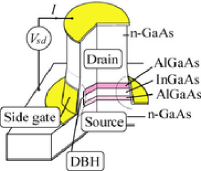
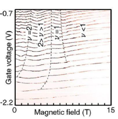
Figure 1: Typical vertical pillar dot (top) and typical transport data (bottom). Labels indicate the Landau level filling factor $\nu$.

A vertical pillar dot (Fig. 1, top frame) consists of a narrow pillar, typically 500 nm in diameter Kouwenhoven01 . The pillar contains a double barrier heterostructure (DBH) which provides confinement in the vertical ($z$) direction and is surrounded by a cylindrical metal gate which carries a negative charge that provides lateral ($x,y$) confinement. The pillar stands on a substrate which is heavily doped and there is also a heavily doped region at the top of the pillar. These heavily doped regions provide source and drain contacts that enable the transport properties of the device to be investigated. A unique advantage of the vertical geometry is that it is not sensitive to edge states which affect transport through lateral devices in the high magnetic field regime.

In a typical experiment, the source-drain current is measured as a function of the gate voltage, $V_{g}$, source-drain voltage, $V_{sd}$ and magnetic field, $B$ parallel to the pillar. Typical results Nishi06 are shown in the bottom frame of Fig. 1. This image shows the condition for an electron to enter the dot at fixed source drain bias. It is well known that transport through the device is Coulomb blockaded except at certain values of $V_{g}$ and $V_{sd}$ Kouwenhoven01 . In Fig. 1 the current is colour coded so that dark regions correspond to the largest current. The $N$th dark curve shows how the gate voltage needed for the $N$th electron to enter the dot depends on the magnetic field. The lowest curve in the figure corresponds to $N=1$.

The exact condition for electron transport is

$$\mu_{c}+\frac{eV_{sd}}{2}\geq\mu_{N}-e\alpha(V_{gN})V_{gN}\geq\mu_{c}-\frac{eV_{sd}}{2},$$ (1)

where $\mu_{c}$ is the contact chemical potential, $V_{gN}$ is the gate voltage at which the $N$th electron enters the dot and $\alpha$ is an electrostatic leverage factor. At zero source drain bias this reduces to

$$e\alpha(V_{gN})V_{gN}=\mu_{N}-\mu_{c}$$ (2)

so that the gate voltage at which transport occurs is a measure of the dot chemical potential relative to the contact. For transport data in the form of a gate voltage difference, $V_{gN}-V_{gN-1}$ is proportional to the addition energy, $E_{AN}=E_{N+1}-2E_{N}+E_{N-1}$ if $\alpha$ and $\mu_{c}$ are independent of $N$. Hence the first and second differences of the dot energies are needed to compare theory with experiment.

II.2 Overview of model

The dot model takes account of vertical confinement, lateral confinement and interactions between dot electrons. The quantum well between the double barriers is relatively narrow (12 nm) so the electrons are confined to the ground state of the vertical motion. This leads to a quasi-two-dimensional model in which the interaction is modified by the vertical confinement, physically the effect is to smear out the Coulomb singularity.

The lateral confinement is generated by the cylindrical side gate and in principle the lateral confinement potential may be found by solving the Poisson equation, refs. Bruce00 ; Matagne02 ; Bednarek03 ; Melnikov05 , for example. However in the present case, $N$ is small so the spatial extent of the dot state ($<50$ nm) is very small compared to the pillar diameter ($\approx 500$ nm). Therefore the only part of the confining potential that has a significant effect on the dot electrons is the part near the minimum which is parabolic. In addition, observation of shell structure in the device considered here Nishi06 shows that the device has a high degree of circular symmetry. The lateral confining potential is therefore taken to be $V_{c}=V_{0}+m^{*}\omega_{0}^{2}r^{2}/2$, where $r$ is the lateral radial co-ordinate and $\omega_{0}$ is found from $\hbar\omega_{0}=a+b(N-1)$ where $a$ and $b$ are fitting parameters. The constant $V_{0}$ is not needed for the present analysis because the addition energy is independent of $V_{0}$ and the chemical potential is also independent of $V_{0}$ when $\mu_{N}$ taken relative to $\mu_{1}$. Previous work has shown that the parabolic approximation is consistent with experiment Maksym90 and accurate for small numbers of electrons Matagne02 , that is electrons in the first and second shells at $B=0$.

The screening is mainly caused by heavily doped contacts that are relatively close to the dot, around 10 nm from the well. This is close enough for the contact regions to have a significant screening effect on the interaction between the dot electrons. This is treated in the Thomas-Fermi approximation and the screening length in the contact region is taken to be a fitting parameter. Full details of the present approach to screening and finite thickness are given in the following two sections.

II.3 Finite thickness

The dot is three dimensional but when the electrons are confined to the vertical ground state their motion is quasi-two-dimensional. A variational method is used to find the resulting effective Hamiltonian. In principle this needs two steps. The envelope function for the vertical confinement should be found first and then the spin splitting should be found from this envelope function Lommer85 . However the second step is not needed here because the experimental value of the effective $g$-factor for the present device is known. Except for the spin splitting terms, the 3D effective mass Hamiltonian is

$$H = \sum_{i}p_{zi}\frac{1}{2m^{*}(z)}p_{zi}+{\bm{\pi}}_{i}\frac{1}{2m^{*}(z)}{\bm{\pi}}_{i}+V_{c}(r_{i})+V_{b}\Theta(z_{i})$$ (3)

$$+ \frac{1}{2}\sum_{i\neq j}U({\bf r}_{i}-{\bf r}_{j},z_{i},z_{j}),$$

where $\mbox{\boldmath{$\pi$}}={\bf p}_{\parallel}+e{\bf A}$, $\bf{p}_{\parallel}$ is the lateral momentum, ${\bf A}$ is the magnetic vector potential, $p_{z}$ is the vertical momentum, $V_{b}$ is the barrier height, $\Theta(z)$ is a step function, $\Theta(z)=1$ when $|z|>w/2$, $\Theta(z)=0$ otherwise, $w$ is the well width, $m^{*}(z)=m^{*}_{w}$ when $z$ is in the well and $m^{*}(z)=m^{*}_{b}$ when $z$ is in the barrier. $U$ is the electron-electron interaction potential and ${\bf r}=(x,y)$. The variational trial function for the electron states is taken to have the form $\Psi=\Pi_{i}\chi(z_{i})\Phi({\bf r}_{1},...{\bf r}_{N})$, where $\Phi$ is antisymmetric and includes spin functions.

Equations for $\Phi$ and $\chi$ are found by minimising $\langle\Psi|H|\Psi\rangle$ subject to the constraint that $\Phi$ and $\chi$ are normalised. This leads to

$$\bar{H}_{\parallel}|\Phi\rangle=\Lambda|\Phi\rangle,$$

$$\left[H_{\perp}+\frac{E_{\parallel}(m^{*}_{b})-E_{\parallel}(m^{*}_{w})}{N}\Theta\right]|\chi\rangle=\Lambda^{\prime}|\chi\rangle,$$ (4)

where $\Lambda$ and $\Lambda^{\prime}$ are eigenvalues, $m^{*}_{w}$ and $m^{*}_{b}$ are effective masses in the well and barrier respectively and $\bar{H}_{\parallel}=p_{w}H_{\parallel}(m^{*}_{w})+(1-p_{w})H_{\parallel}(m^{*}_{b})$. Here $p_{w}$ is the probability of finding and electron in the well, $p_{w}=\int^{w/2}_{-w/2}\chi^{2}(z)dz$ and the parallel and perpendicular Hamiltonians are defined by

$$H_{\parallel}(m) = \sum_{i}\frac{\pi^{2}_{i}}{2m}+V_{c}(r_{i})$$

$$+ \frac{1}{2}\sum_{i\neq j}\int\chi^{2}(z)\chi^{2}(z^{\prime})U({\bf r}_{i}-{\bf r}_{j},z,z^{\prime})dzdz^{\prime},$$

$$H_{\perp} = p_{z}\frac{1}{2m^{*}(z)}p_{z}+V_{b}\Theta(z).$$ (5)

The parallel energies in the second of Eqs. (4) are expectation values of $H_{\parallel}$: $E_{\parallel}(m)=\langle\Phi|H_{\parallel}(m)|\Phi\rangle$. After Eqs. (4) have been solved the total energy is found from the expectation value of the full Hamiltonian:

$$E=N\langle\chi|H_{\perp}|\chi\rangle+\langle\Phi|\bar{H}_{\parallel}|\Phi\rangle.$$ (6)

In principle, the coupled eigenvalue problem defined by Eqs. (4) can be solved iteratively to arbitrary accuracy but in practice this is not necessary. The energy difference term $[E_{\parallel}(m^{*}_{b})-E_{\parallel}(m^{*}_{w})]/N$ in the second of Eqs. (4) in the present case is around 1% of the barrier height. Hence the effect of this term is small and it is sufficient to find $\chi$ from the zeroth-order approximation in which the energy difference term is neglected and then use the zeroth-order $\chi$ to find the averaged Hamiltonian $\bar{H}_{\parallel}$. The averaging has two physical effects. First, it changes the effective mass. The dot considered here is made from InGaAs containing 5% In, and the In reduces the mass. The barrier is made from AlGaAs containing 22% Al and this increases the mass. The net effect is to reduce the mass to $0.0653m_{0}$, slightly less than the GaAs value. The second effect of the averaging is to smear out the Coulomb singularity in the effective two-dimensional interaction. This results from the integral over $z$ in the first of Eqs. (5). The averaging procedure also applies to systems with spin-orbit coupling. In this case, it is found that the Dresselhaus spin-orbit coupling parameter has to be averaged in a way similar to the effective mass. This has been used for studies of spin relaxation in the present device Chaney07 .

The final step in determining the effective Hamiltonian is to find the spin splitting. The effective $g$-factor, $|g^{*}|$, is determined from the experimentally observed Zeeman splitting Nishi06 in the same device that is used for the data analysis performed here. $|g^{*}|=0.3$ for the dot when $B\gtrsim 10$ T, compared with $|g^{*}|=0.44$ for bulk GaAs. The reduced value for the dot is consistent with the effect of non-parabolicity Lommer85 . The non-parabolicity also makes the effective $g$-factor depend on magnetic field and Landau level index Lommer85 but the resulting corrections to $\mu_{N}$ are probably smaller than experimental error. A constant $g$-factor is therefore used and the Zeeman energy is accounted for by adding $g^{*}\mu_{B}BS_{z}$ to the total energy in Eq. 6. Here $\mu_{B}$ is the Bohr magneton and $S_{z}$ is the $z$ component of the total spin $S$. The effective $g$-factor is assumed to be negative, as in bulk GaAs, so $g^{*}=-0.3$.

II.4 Screening

The most important source of screening in the present device is the heavily doped contacts above and below the dot. The dielectric response of the disordered contact material is not well understood but can be treated approximately in the static Thomas-Fermi approximation. This allows the screening length to be estimated from the density of states at the Fermi level, however this is not known accurately for the contact material. Hence the screening length is taken to be a fitting parameter which is determined from experimental data.

The screened interaction between dot electrons Hallam96 is found from the electrostatic Green’s function $G({\bf R},{\bf R}^{\prime})$ which satisfies

$$-\mbox{\boldmath{$\nabla$}}\cdot\left[(\epsilon({\bf R})\epsilon_{0}\mbox{\boldmath{$\nabla$}}G({\bf R},{\bf R}^{\prime})\right] = -q_{0}^{2}({\bf R})\epsilon({\bf R})\epsilon_{0}G({\bf R},{\bf R}^{\prime})$$ (7)

$$+ \delta({\bf R}-{\bf R}^{\prime}),$$

where $\epsilon({\bf R})$ is the relative permittivity, $q_{0}=2\pi/\lambda_{s}$ inside the contacts, $q_{0}=0$ outside the contacts and ${\bf R}=({\bf r},z)$. Because a detailed theory of magnetic field dependent screening by the 3D contact material is not available, the screening length, $\lambda_{s}$, is taken to be independent of the magnetic field. This approximation should be good when the screening length does not change significantly over the field range used in the experiments and it is assumed that this is the case. Eq. (7) is simplified by making use of the fact that the dot is an order of magnitude smaller than the pillar. This means that the Green’s function is almost translationally invariant in the lateral direction and can be found to a good approximation by replacing the pillar by a stack of dielectric layers of infinite extent in the lateral directions. $\epsilon$ and $q_{0}$ then do not depend on ${\bf r}$. So the Green’s function is translationally invariant in the lateral directions and can be expressed as a Fourier transform:

$$G({\bf R},{\bf R}^{\prime})=\frac{1}{4\pi^{2}}\int G({q},z,z^{\prime})\exp(i{\bf q}\cdot({\bf r}-{\bf r}^{\prime}))d{\bf q}.$$ (8)

The Fourier components of the Green’s function satisfy

$$- \frac{d}{dz}\left[\epsilon(z)\epsilon_{0}\frac{d}{dz}G({q},z,z^{\prime})\right]$$ (9)

$$+ \epsilon(z)\epsilon_{0}[q^{2}+q^{2}_{0}(z)]G({q},z,z^{\prime})=\delta(z-z^{\prime}).$$

The solution of this equation has the form

$$G({q},z,z^{\prime})=-\frac{f(z)g(z^{\prime})}{W},\qquad z>z^{\prime},$$

$$G({q},z,z^{\prime})=-\frac{g(z)f(z^{\prime})}{W},\qquad z<z^{\prime},$$ (10)

where $f$ and $g$ are solutions of the homogeneous equation corresponding to Eq. (9) and $W$ is their Wronskian. These solutions are chosen to satisfy $f\rightarrow 0$ when $z\rightarrow+\infty$ and $g\rightarrow 0$ when $z\rightarrow-\infty$. Although the analytic form of $G$ is as given in Eq. (10), severe numerical instabilities are encountered when this form is evaluated unless special precautions are taken. The problem is that the $G$ has rapidly growing components which cause exponent overflow. Exactly the same mathematical problem is encountered in calculations of evanescent wave propagation in electron diffraction theory and the solution used here is a reflection matrix approach developed for calculations of reflection high energy electron diffraction (RHEED) Meyer-Ehmsen89 ; Zhao93 ; Kawamura07 . This is detailed in appendix A.

Once the Green’s function has been found, the Fourier components of the effective two-dimensional interaction are obtained in the form of an integral:

$$U_{2d}(q)=e^{2}\int\chi^{2}(z)\chi^{2}(z^{\prime})G({q},z,z^{\prime})dzdz^{\prime}.$$ (11)

The special form of the Green’s function, Eq. (10), is used to simplify this integral so that it can be evaluated efficiently. Details are given appendix B. The form of the effective interaction in real space is very different from a pure Coulomb interaction. Because of the screening, the interaction is dipole-like at long range and decreases like $1/r^{3}$ in the limit of large $r$. And the Coulomb singularity is removed by the finite thickness because the electrons are able to move out of the dot plane and avoid each other. The real-space effective interaction as a function of $r$ is shown in Fig. 2. $U_{2d}(r)$ is calculated numerically from its Fourier transform $U_{2d}(q)$ for the layer structure shown in Fig. 1 (see also Table 1) and $\lambda_{s}=10$ nm, a typical screening length. The length unit is the 2D harmonic oscillator length parameter, $\lambda^{2}=\hbar/(2m^{*}\Omega)$ where $\Omega^{2}=\omega_{0}^{2}+\omega^{2}_{c}/4$ with $\omega_{c}$ the cyclotron frequency. The energy unit $E_{\lambda}=e^{2}/(4\pi\epsilon_{w}\epsilon_{0}\lambda)$ where $\epsilon_{w}$ is the relative permittivity in the well that contains the dot.

Figure 2: Effective 2D interaction (solid line). Dashed lines show the $1/r^{3}$ limiting form and the $1/r$ Coulomb interaction.

It is clear that $U(r)$ is significantly different from the $1/r$ Coulomb interaction and approaches the $1/r^{3}$ form in the limit of large $r$.

The effect of the dielectric interfaces in the device on the effective interaction is accounted for fully in the Green’s function formalism. In addition, the dielectric interfaces have an effect on the vertical confinement potential. This results from the interaction of each electron with its own image charges and is also accounted for in the Green’s function formalism. The image charge contribution to the vertical confinement is obtained from the non-singular part of the Green’s function Hallam96 and in the present case the image charge contribution is

$$V_{I}(z) = \frac{e^{2}}{8\pi\epsilon_{w}\epsilon_{0}}\int^{\infty}_{0}\left[2q\epsilon_{w}\epsilon_{0}G(q,z,z)-\frac{\epsilon_{w}}{\tilde{\epsilon}}\right]d{q},$$ (12)

where $\tilde{\epsilon}=\epsilon_{w}$ when $z$ is in the well, $\tilde{\epsilon}=\epsilon_{b}$, the barrier relative permittivity, when $z$ is in the barrier and $\tilde{\epsilon}=(\epsilon_{w}+\epsilon_{b})/2$ when $z$ is at the interface between the well and the barrier. The image charge term leads to a small change in the vertical confinement which is taken into account via perturbation theory.

Another source of screening in the present device is the metallic, cylindrical side gate. In principle, this breaks the translational invariance of the effective lateral interaction however this effect is expected to be small. The magnitude of the effect can be estimated from the electrostatic Green’s function for an infinite metallic cylinder Smythe68 . Numerical calculations of the Green’s function suggest that the effect is $\lesssim 1$% within a region of radius $\sim 10$ nm in the centre of the cylinder. The effect is clearly largest for electrons at the edge of the dot but the interaction between these electrons and electrons in the centre of the dot is suppressed by the screening effect of the contacts. These considerations suggest that the effect of the gate is small for the small electron numbers considered here ($N\leq 5$). However, the effect could be significant for larger electron droplets whose edge is closer to the metallic gate.

II.5 Model Hamiltonian

Table 1: Layer structure of the device model.

Layer	Composition	Thickness
Top contact	n+ GaAs
Buffer	i GaAs	3 nm
Barrier	Al0.22Ga0.78As	9 nm
Well	In0.05Ga0.95As	12 nm
Barrier	Al0.22Ga0.78As	7.5 nm
Buffer	i GaAs	3 nm
Bottom contact	n+ GaAs

Table 2: Material parameters for the device model.

Parameter	Material	Value
$m^{*}/m_{0}$	AlxGa1-xAs	$0.067+0.083x$
$m^{*}/m_{0}$	InyGa1-yAs	$0.067-0.045y$
$V_{b}$ (meV)	AlxGa1-xAs / InyGa1-yAs	$823x+640y$
$\epsilon_{b}$	AlxGa1-xAs	$12.7-3.12x$
$\epsilon_{w}$	InyGa1-yAs	$12.7+2y$

The effective Hamiltonian for the two-dimensional dot model is

$$H_{eff} = \sum_{i}\frac{\pi^{2}_{i}}{2\bar{m}^{*}}+V_{c}(r_{i})+NE_{z}+g^{*}\mu_{B}BS_{z}$$ (13)

$$+ \frac{1}{2}\sum_{i\neq j}U_{2d}({\bf r}_{i}-{\bf r}_{j}),$$

where $E_{z}=\langle\chi|H_{\perp}|\chi\rangle+\Delta V_{I}$ is the perpendicular energy, $\Delta V_{I}$ is the perturbation caused by the image charge term. The averaged effective mass $\bar{m}^{*}$ is found from $1/\bar{m}^{*}=p_{w}/m^{*}_{w}+(1-p_{w})/m^{*}_{b}$ and the effective $g$-factor is determined experimentally (Section II.3). The layer structure of the device is detailed in Table 1 and the material parameters used for the present calculations are detailed in Table 2.

III Calculation of Eigenstates

The effective Hamiltonian $H_{eff}$ is very similar to the Hamiltonian for a two dimensional parabolic dot with a Coulomb interaction. Hence the eigenstates of $H_{eff}$ are found in the usual way by numerical diagonalization in a Fock-Darwin basis Chakraborty99 . The only difference between the usual calculation and the present one is that matrix elements of the effective interaction $U_{2d}$ have to be computed. In the case of the Coulomb interaction these matrix elements are normally found from the Fourier transform of the interaction and the calculation involves an integral over $q$ Chakraborty99 . In the present case the Fourier transform approach is also used. $U_{2d}(q)$ has the form $F(q)V_{2d}(q)$ where $V_{2d}(q)$ is the Fourier transform of the Coulomb interaction, $e^{2}/(4\pi\epsilon_{w}\epsilon_{0}r)$, in two dimensions and $F(q)$ is a form factor that is computed numerically from the Green’s function. The only difference between the standard treatment of the interaction in a 2D dot and the present treatment is the appearance of the form factor in the $q$ integral. This integral is done numerically by Romberg integration.

The Fock-Darwin states are labelled by an angular momentum quantum number $l$ and a radial quantum number $n$. The many-electron basis used for the diagonalization consists of Slater determinants formed from these states. It is important to minimise the size of this basis as expensive calculations have to be performed repeatedly to fit the model parameters. The Hamiltonian is block diagonalized according to the value of the total orbital angular momentum $J$. For $N\leq 4$ the basis for each $J$ is formed from Fock-Darwin states with $n\leq 3$ and all $l$ values compatible with the required $J$ value. For $N=5$ the size of the basis is limited by making use of the fact that the radial excitation is an inter-Landau level excitation and hence has large energy in a strong magnetic field. This enables the maximum $n$ quantum number to be reduced as a function of magnetic field. In the present case the maximum value of $n$ is taken to be the integer part of $6.9-0.28B$ which corresponds to a maximum $n$ of 6 at $B=0$ T and 2 at $B=14$ T. All Slater determinants compatible with this $n$ value are then constructed and those Slater determinants whose energy is within 100 meV of the lowest energy determinant are retained in the calculation. This rejection step reduces the total number of determinants slightly and saves some computer time. The accuracy of the numerically calculated ground state addition energies is estimated to be 0.1 meV or better. The $B$-dependent cut-off on $n$ leads to small steps in the energy as a function of $B$ which result from the sudden change in the number of basis states that occurs whenever the integer part of $6.9-0.28B$ changes. These artefacts are typically around 0.01 meV, about an order of magnitude smaller than experimental error.

IV Data Analysis

IV.1 Parameter fitting

Standard techniques are used to fit the model parameters. The general idea is to find parameters that minimise the metric distance between experimental and theoretical curves. This problem occurs in many areas of physics and the present work is based on a formalism developed for surface structure analysis Stock90 ; Coy98 . For each curve, the metric distance is taken to be

$$D=\frac{1}{N_{p}}\sum_{i}\left[f_{t}(B_{i})-f_{e}(B_{i})\right]^{2},$$ (14)

where $f_{t}$ and $f_{e}$ are theoretical and observed values of the addition energy or chemical potential at magnetic field $B_{i}$ and $N_{p}$ is the number of experimental points in the curve. The metric distance used to fit multiple curves is the average of the metric distances for the individual curves weighted with the number of points in each curve. With this choice, the procedure reduces to an unweighted least squares fit of the entire data set. It is possible to adjust the metric to give weight to specific features in the data, such as peaks and shoulders, but this is not done in the present work. The metric distance is minimised with the Levenberg-Marquardt algorithm, a standard numerical technique Press93 . This fitting procedure is generally accepted to give reliable parameter values provided the number of features in the data exceeds the number of fitting parameters, a condition that is satisfied in the present case.

IV.2 Analysis of addition energy data

The addition energy data was collected as part of an experiment to investigate ground state transitions in the high-magnetic field regime Nishi06 . The data was taken with a fairly high magnetic field resolution (0.05 T) and consists of a limited number of $V_{gN}$ curves, $N=2,3,4,5$ only. The measurements were performed in a dilution refrigerator and the electron temperature is estimated to be below 100 mK.

Figure 3: Experimental and theoretical addition energies. The field range used for parameter fitting is $0\leq B\leq 14$ T. Diamonds: experimental data, solid lines: theoretical results.

Figure 4: Experimental and theoretical addition energies. As Fig. 3 except that the field range used for parameter fitting is $0\leq B\leq 10$ T.

The ground state addition energy is the difference of two successive chemical potentials: $E_{AN}=E_{N+1}-2E_{N}+E_{N-1}=\mu_{N+1}-\mu_{N}$. It follows from Eq. (2) that $E_{AN}$ at fixed magnetic field is related to two successive gate voltages:

$$E_{AN}=e[\alpha(V_{gN+1})V_{gN+1}-\alpha(V_{gN})V_{gN}],$$ (15)

which is valid provided that the contact chemical potential $\mu_{c}$ is independent of $V_{g}$ and therefore cancels when the $\alpha V_{g}$ values are subtracted. Eq. (15) can in principle be used to find $E_{AN}$ from experimental values of $\alpha$ and $V_{g}$. However this requires very accurate values of both $\alpha$ and $V_{g}$. Typical values of $E_{AN}$ are around 3 meV, while typical values of $e\alpha V_{g}$ are around 60 meV. So both $\alpha$ and $V_{g}$ need to be measured to an accuracy of 0.1 % or better to measure $E_{AN}$ to $\pm 0.1$ meV. $V_{g}$ is known to this accuracy for the present device but $\alpha$ is not. Eq. (15) is therefore approximated by

$$E_{AN}=e\bar{\alpha}_{N+1}(V_{gN+1}-V_{gN}),$$ (16)

where $\bar{\alpha}_{N+1}=[\alpha(V_{gN+1})+\alpha(V_{gN})]/2$. This suppresses the random errors which would result from use of Eq. (15) but is only valid when $\alpha(V_{gN})$ varies sufficiently slowly with $N$. This is assumed to be the case. The validity of this assumption cannot be tested without more data on $\alpha$ however the results based on this assumption are found to be consistent with results of chemical potential analysis, section IV.3. Another factor that limits the present analysis is that $\alpha$ depends on the magnetic field as well as $V_{g}$ but is only known for a sample of field points at intervals of around $1-2$ T. The $\alpha$ values at intermediate field points have to be obtained by linear interpolation and this introduces a further systematic error which is difficult to quantify. In principle, both this systematic error and the one resulting from use of $\bar{\alpha}$ can be eliminated by performing detailed measurements of $\alpha$.

Figure 3 shows the comparison between experimental and theoretical addition energies for $N=2$, 3, 4. All three curves were used simultaneously to fit the parameters, as described in section IV.1. It is clear that the absolute values of the experimental and theoretical data agree very well. The raw experimental data is shown in the figure together with raw theoretical data. There is no shifting or scaling of the theoretical curves. The agreement is generally good but there are some discrepancies, particularly around 4-6 T and above 10 T. To investigate the cause of these discrepancies the data was fitted again in the restricted field range $0\leq B\leq 10$ T. The results are shown in Fig. 4 and it is clear that the fit is better, particularly around 4-6 T where the double peak structure for $N=3$ and $N=4$ is reproduced very well. The improvement in the fit can be quantified with the metric distance which is equivalent to the RMS difference between experiment and theory. The value corresponding to Fig. 3 is 0.23 meV while for Fig. 4 it is 0.15 meV.

The deterioration in the quality of the fit when the full data range is used could be caused by factors not included in the model or uncertainties in the experimental data. The most likely causes are impurity effects, screening and insufficient knowledge of $\alpha$.

Both impurity effects and screening could depend on magnetic field. Impurity effects are not included in the present model but are likely to be more significant in the very strong field regime. The mean distance between the impurities in the heavily doped contacts is around 10 nm. This gives a fluctuating contribution to the dot potential on a similar length scale. But at zero magnetic field the typical diameter of the dot state is around 20 - 30 nm. Hence the effect of the impurities will tend to average out. Indeed the experimental evidence is that the present device has a high degree of circular symmetry Nishi06 . However as the magnetic field increases the dot wave function shrinks and eventually becomes smaller than the length scale of the potential fluctuations. Impurity effects would be large in this regime but the magnetic fields used in the present work are probably too low for this to happen. Magnetic field dependent screening is another possible cause of discrepancies but if the magnetic field dependence was significant, it would probably occur throughout the field range, while the discrepancies are mainly in the high field range.

The remaining possible cause of the discrepancies is that the value of $\alpha$ is not known to sufficient accuracy in the high-field regime. In this case the parameters determined by fitting the data up to 10 T are expected to provide an accurate description of the dot in the field range up to 14 T but the problem lies in the numerical value of the experimental addition energy. There is some evidence that this is the case: excited state features predicted by the present model are found to correspond to features in experimental excitation spectra in the high-field regime Nishi06 . The value of $\alpha$ is not needed to identify these features and this suggests that the discrepancies in the high field addition energy are most likely to be related to insufficient knowledge of $\alpha$.

The best fit parameter values corresponding to Fig. 4 are $a=4.8\pm 0.1$ meV, $b=0.02\pm 0.01$ meV and $\lambda_{s}=15.0\pm 3$ nm. Here the statistical errors correspond to the parameter range compatible with the fluctuations in the data shown in Fig. 4 but exclude the unquantifiable uncertainty in $\alpha$. These values are taken to give the best model of the present device. The value of $b$ suggests that the confinement energy increases slowly with gate voltage but the opposite would be expected from electrostatics of the device. However the value of $b$ is comparable to its error so a model with constant confinement or slowly decreasing confinement would probably give an equally good fit to the data.

IV.3 Analysis of chemical potential data

In principle, Eq. (2) can be used to obtain $\mu_{N}$ from the $V_{g}$ data but the appearance of the contact chemical potential $\mu_{c}$ in this equation presents an obstacle. The absolute value of $\mu_{c}$ is not known. In addition, $\mu_{c}$ is expected to vary with magnetic field and its field dependence is not known. Part of the difficulty can be eliminated by taking the chemical potential relative to the chemical potential for the first electron at zero magnetic field. The contact chemical potential is written as $\mu_{c}(0)+\Delta\mu_{c}(B)$, where $\Delta\mu_{c}$ vanishes when $B=0$. Eq. (2) becomes

$$e[\alpha(V_{gN},B)V_{gN}(B)-\alpha(V_{g1},0)V_{g1}(0)] =$$

$$\mu_{N}(B)-\mu_{1}(0)-\Delta\mu_{c}(B).$$ (17)

This enables experimental and theoretical values of $\mu_{N}(B)-\mu_{1}(0)$ to be compared provided that a model for $\Delta\mu_{c}(B)$ is available. A model investigated in the present work is $\Delta\mu_{c}(B)=\sqrt{\Gamma^{2}+(\hbar\omega_{c}/2)^{2}}-\Gamma$, where $\Gamma$ is a fitting parameter. An advantage of analysing chemical potential data is that Eq. (17) is less sensitive to errors in $\alpha$ than Eq. (15) however the disadvantage is that the results depend on the model chosen for $\Delta\mu_{c}(B)$.

Chemical potential data analysis requires a data set that contains $V_{g1}$ so that $\mu_{N}(B)-\mu_{1}(0)$ can be found. The addition energy data analysed in section IV.2 does not contain $N=1$ data so a second data set is used for the chemical potential data analysis. This data was collected under similar conditions to the addition energy data but over a wider range of $N$, a smaller magnetic field range and a lower field resolution (0.1 T). In addition, the device was subjected to one thermal cycle between collecting the two data sets. The chemical potential data was collected first then the device was taken up to room temperature and cooled again to collect the addition energy data.

Figure 5: Experimental and theoretical chemical potentials. Diamonds: experimental data, solid lines: theoretical results.

The comparison between experimental and theoretical chemical potentials is shown in Fig. 5. As with the addition energy, a very good fit is obtained without any scaling or shifting of the theoretical data. The RMS difference between the experimental and theoretical curves is about 0.12 meV. The best fit parameter values are $a=4.8\pm 0.1$ meV, $b=-0.06\pm 0.02$ meV, $\lambda_{s}=16.0\pm 2$ nm and $\Gamma=7.4\pm 0.3$ meV. Except for the sign of $b$, these values are consistent with the values obtained by fitting the addition energy. As with the addition energy the absolute magnitude of $b$ is small and the statistical error in $b$ is relatively large. This suggests that the variation of $\hbar\omega_{0}$ with $N$ is not very significant for the small $N$ range considered here.

The best model of the device is believed to be the model that results from fitting the addition energy because an extra parameter is needed to fit the chemical potential data and it is preferable to keep the number of fitting parameters to a minimum. The addition energy model was therefore used in ref. Nishi06 to determine ground state quantum numbers from transport data. However ref. Nishi06 contains excited state data and comparison of features in experimental and theoretical excitation data requires comparison of chemical potential data. This appears to be an insurmountable problem because the addition energy data does not contain $V_{g1}(B)$ so it is impossible to fit $\Gamma$ for the experimental conditions of ref. Nishi06 . However, the exact value of the chemical potential is not needed for the analysis of ref. Nishi06 and similar situations because the only information that needs to be extracted from the experimental and theoretical data is the magnetic fields at which features occur. As an aid to identification of these features it is very useful to compute the chemical potential as $\mu_{N}(B)-\mu_{1}(0)-\Delta\mu_{c}(B)$ because this ensures that the experimental and theoretical data have roughly the same slope. This can be achieved by using an approximate value of $\Gamma$ that is found by visual comparison of the data, $8.2$ meV in the case of ref. Nishi06 . The precise value of $\Gamma$ is not important in this case as $\Gamma$ does not affect the position of features in the transport data.

V Applications of the model

V.1 Low field data

Figure 6: Experimental and theoretical excitation spectra. Left frame: experimental excitation spectra. The grey scale image shows $dI_{sd}/dV_{g}$ in the $B,V_{g}$ plane for $N=1$-6. Right frame: theoretical excitation spectra for $N=2$-5. The dashed lines show the upper bound of the excitation stripe, $\Delta E=2$ meV. Roman font labels indicate the features listed in Table 3.

Table 3: Comparison of features in experimental and theoretical spectra. Features (a), (d), (e) and (j) are ground state transitions. For these features $(L,S)\rightarrow(L^{\prime},S^{\prime})$ indicates low field values of $(L,S)$ followed by high field values. Features (b), (f), (g) and (h) are excitation energies at the points shown in Fig. 6 and defined in the text. Feature (c’) is the excitation energy on line (c) at $B=3.0$ T. For these features $(L,S)\Rightarrow(L^{\prime},S^{\prime})$ indicates excited state $(L,S)$ values followed by the ground state values.

Feature	$N$	$\Delta E_{Exp}$ (meV)	$\Delta E_{The}$ (meV)	$B_{Exp}$ (T)	$B_{The}$ (T)	$(L,S)$ values
(a)	2	0.0	0.0	3.8	4.2	$(0,0)\rightarrow(1,1)$
(b)	2	2.0	2.0	0.75	1.15	$(1,1)\Rightarrow(0,0)$
(c’)	3	1.4	1.22	3.0	3.0	$(3,\frac{3}{2})\Rightarrow(1,\frac{1}{2})$
(d)	4	0.0	0.0	0.33	0.3	$(0,1)\rightarrow(2,0)$
(e)	4	0.0	0.0	4.06	4.0	$(2,0)\rightarrow(3,1)$
(f)	4	1.0	1.24	0.0	0.0	$(0,0)\Rightarrow(0,1)$
(g)	4	2.0	2.0	0.86	0.70	$(0,0)\Rightarrow(2,0)$
(h)	4	1.5	1.71	1.57	1.3	$(0,1)\Rightarrow(3,1)$
(j)	5	0.0	0.0	1.39	1.25	$(1,\frac{1}{2})\rightarrow(4,\frac{1}{2})$

The model parameters are found by fitting to the ground state addition energies so comparison of theoretical and experimental excitation energies is a good test of the predictive power of the model. This comparison is performed here for the low magnetic field regime, $B\leq 5$ T, to which the model has not been applied before. A discussion of the high field regime is available in the literature Nishi06 , see also section V.2.

The experimental excitation energy data Fig. 6 (left panel) consists of the derivative of the source-drain current, $dI_{sd}/dV_{g}$, plotted as an intensity image in the $B,V_{g}$ plane. The electron number ranges from 1 to 6. The data was collected in a similar way to the addition energy data but during a different thermal cycle. The source-drain voltage $V_{sd}=2$ mV so the maximum excitation energy that can be probed is 2 meV. For each electron number there is a stripe that corresponds to this 2 meV window. The width of each stripe depends on $B$ and $V_{g}$ because of the $B$ and $V_{g}$ dependence of $\alpha$. Within each strip there are dark lines that correspond to transport through excited dot states. The excitation energy is found by scaling the line position to the stripe width. This gives excitation energies, $\Delta E$, to an accuracy of about $\pm 0.1$ meV, together with field values accurate to about $\pm 0.02$ T. In addition to the excitation lines, there is ’noise’. Some of this is caused by emitter states which result from density of states fluctuations in the heavily doped contacts. To extract the $B$ dependence of the excitation lines it is necessary to distinguish contact features from dot features. This can be done by rejecting features that do not depend on $N$ Nishi06 , for example. However the excitation lines in Fig. 6 have gaps and are of variable intensity so the present quantitative comparison is based on features like level crossings and crossings of excitation lines with the upper boundaries of the excitation stripes. These features can be identified unambiguously by comparing the topology of the experimental and theoretical data.

The theoretical excitation energy data is shown in the right frame of Fig. 6. The figure shows $\mu_{N}(B)-\mu_{1}(0)-\Delta\mu_{c}(B)$ for electron numbers in the range 2 to 5. For each $N$ the energies of the ground state and lowest four excited states are calculated and the value of $\mu_{N}(B)-\mu_{1}(0)-\Delta\mu_{c}(B)$ is found for the ground state and each of the excited states. The excited state lines that fit into the 2 meV excitation window are shown by the solid lines in the figure. The continuous solid line at the bottom of each stripe is the ground state chemical potential and this coincides with the lower boundary of each excitation window. The dashed line at the top of each stripe shows the upper boundary, 2 meV above the ground state line.

Qualitatively, there is very good agreement between the theory and experiment. However some of the experimental excited state lines are not continuous and there is some noise. The singlet-triplet transition of the 2 electron system is clearly visible (a) and so is the excited state triplet line (b-a). For 3 electrons there are ground state transitions in the 4-5 T interval in both the theory and experiment and an excited state line is visible in the experimental data. This probably corresponds to line (c) in the theory. In the case of 4 electrons there are ground state transitions (d) and (e) in both theory and experiment. In addition, an excited state line which has a flat maximum is present in the experimental data. This corresponds to the crossing (h) in the theory but small symmetry breaking effects such as disorder change the crossing into an anticrossing and lead to a maximum in the experimental data. The second excited state line (f-g) is also clearly visible in both the theory and experiment. For 5 electrons the ground state transition (j) has the distinctive form of a maximum and is clearly present in both theory and experiment, and some short excited state lines emerge from this crossing. Further, for both 4 and 5 electrons the experimental ground state line is broadened in the regions between 4 and 5 T. This corresponds to the region where the theory predicts that ground and excited state levels cluster together and excitation gaps shrink. Although the agreement is generally good, there are some discrepancies. For $N=1$ the theory predicts no excitations within the 2 meV window at fields below 5 T but there is some structure in the experimental data. This is thought to be caused by emitter states. Similarly, for $N=5$ no excitations are predicted in the 2 meV window at zero magnetic field but there is some structure in the data.

The quantitative experiment-theory comparison for features (a)-(j) is detailed in Table 3. For each feature, experimental and theoretical values of $\Delta E$ and $B$ are given but $\Delta E=0$ in the case of ground and excited state transitions. The theoretical magnetic fields are accurate to about 0.05 T, the magnetic field step used for the calculations. The theoretical quantum numbers are also listed. In the case of excitations ($\rightarrow$), the quantum numbers of the excited state are shown followed by those of the ground state. In the case of ground state transitions ($\Rightarrow$), the quantum numbers on the low field side of the transition are followed by those on the high field side.

In the case of the singlet-triplet transition of the 2-electron system (a), the predicted transition field is about 0.4 T lower than in the experiment and the point where the triplet excitation line crosses the 2 meV excitation boundary (b) is also about 0.4 T lower. This discrepancy is thought to be a consequence of the thermal cycling since the positions of the singlet-triplet transition agree well in the addition energy data, Fig 4. The excited state line of the 3-electron system (c) is difficult to identify because it is not clear whether it extends as far as the excitation boundary in the experimental data. However there is some weak excited state structure in the data at around 3.5 T and this suggests that the experimental line is the second excited state. The experimental excitation energy is compared with the theoretical second excited state energy at the arbitrarily chosen field of 3 T in Table 3 (feature (c’)). The two values differ by only 0.18 meV and this supports the idea that the experimental line is the second excited state. In addition, the extrapolation of the experimental line crosses the upper boundary of the excitation stripe at about 2.24 T compared with 2.4 T in the theory and line (c) crosses the theoretical ground state line at 4.6 T close to an experimental ground state transition at 4.58 T. This gives further support to the interpretation of the experimental excited state line as the second excited state line corresponding to theoretical line (c).

The 4-electron system is rich in features that can be identified unambiguously and compared quantitatively with theory. Ground state transitions at 0.33 and 4.06 T agree very well with transitions at 0.3 T (d) and 4.0 T (e) in the theory. The excitation energy of the second excited state (f) at zero magnetic field agrees with theory to 0.24 meV while the position of the crossing of the second excited state line with the excitation stripe boundary (g) agrees with theory to 0.16T. The excitation energy at the excited state crossing (h) agrees to 0.21 meV and its position agrees to 0.27 T. It is more difficult to identify features in the 5-electron data as there is more noise. However the position of the ground state transition (j) agrees to 0.14 T.

V.2 High field data

Application of the present model to data in the high magnetic field regime beyond the MDD has been discussed in ref. Nishi06 . However the fitting procedures described here are not detailed in that work. Here it is emphasised that identical procedures were used in the present work and the work described in ref. Nishi06 and that identical model parameters were used in both cases. One of the main findings of ref. Nishi06 is the existence of intermediate spin states in the regime beyond the MDD. The MDD is spin polarised but as the magnetic field increases a transition to a partly polarised state occurs, followed by a spin polarised state, then another partly polarised state and so on. The quantum numbers found for the $N=5$ dot studied in ref. Nishi06 are consistent with general ideas about symmetry and electron molecular states Maksym96 ; Maksym00 . In the specific case of the $N=5$ partly polarised states, calculations of the pair correlation function indicate that there is a superposition of 4- and 5-fold symmetry with a dominant 5-fold component. Further details are given in refs. Maksym06 ; MaksymArita07 .

VI Conclusion

An accurate model of a vertical pillar quantum dot has been developed which is able to reproduce addition energy and chemical potential data for individual quantum dots. Experimental addition energies are reproduced to an accuracy of around 0.15 meV and this is accurate enough to enable ground state spin and orbital angular momentum quantum numbers to be determined from transport data. Although the three-dimensional device structure is accounted for, the resulting physical model reduces to one in which electron motion is restricted to the two lateral dimensions, the confinement is parabolic and the interaction potential differs significantly from the bare Coulomb potential.

The model only contains 3 adjustable parameters. Of these the parameter that describes the $N$ dependence of the confinement energy does not appear to be significant over the small $N$ range considered here and it is likely that a two parameter model would give similar accuracy to the present one. For dots with larger $N$ it would be possible to include non-parabolic confinement. This would increase the number of model parameters but with larger $N$ there would be more data so the additional parameters could probably be determined reliably.

Although the model parameters are determined by fitting ground state data, the model is able to give a good description of the low lying excited states. The model energies agree with experiment to about 10-20% and the positions of features in magnetic field dependent data agree to similar accuracy. One of the factors limiting the accuracy of the present analysis is uncertainty in the value of the electrostatic leverage factor $\alpha$. Accurate measurements of $\alpha$ would enhance the scope and applicability of the present analysis.

The general approach described here is not limited to vertical pillar dots. In principle, similar analysis procedures could be developed for any type of dot, provided a good physical model is available.

Appendix A Numerical calculation of Green’s function

The functions $f$ and $g$ and the Wronskian $W$ (Eq. 10) are needed to find the Green’s function. To find $f$ and $g$ the system is divided into thin slices, such that $\epsilon$ and $q_{0}$ are constant in each slice. In the present case this simply means that each layer of the structure is sub-divided into thin slices but the same numerical procedure is applicable to any form of $\epsilon(z)$. The $n$th slice occupies the region between $z_{n-1}$ and $z_{n}$ and is characterised by a relative permittivity $\epsilon_{n}$, $q$ value $q_{n}^{2}=q^{2}+q_{0}^{2}(z)$ and a thickness $t_{n}=z_{n}-z_{n-1}$. Within each slice $f$ and $g$ have the form $A_{n}\exp(-q_{n}z)+B_{n}\exp(q_{n}z)$. The two terms in this expression are analogous to evanescent waves in diffraction theory and it is convenient to use the language of diffraction theory to describe them. Thus the reflected wave, $R$ which decays in the positive $z$ direction has the form $R=A_{n}\exp(-q_{n}z)$. Similarly, the transmitted wave, $T$ which decays in the negative $z$ direction has the form $T=B_{n}\exp(q_{n}z)$.

The amplitudes at successive slices are related via a transfer matrix,

$$\left(\begin{array}[]{c}R_{n+1}\\ T_{n+1}\\ \end{array}\right)=\left(\begin{array}[]{cc}m_{1}&m_{2}\\ m_{3}&m_{4}\\ \end{array}\right)\left(\begin{array}[]{c}R_{n}\\ T_{n}\\ \end{array}\right),$$ (18)

where $R_{n}$ and $T_{n}$ are amplitudes just below the interface at $z_{n}$, that is within the slice of relative permittivity $\epsilon_{n}$. The boundary conditions on $G$ are used to find the elements of the transfer matrix: $g$ and $\epsilon(z)dg/dz$ are continuous and the same holds for $f$. Therefore

$$m_{1} = \frac{1}{2}\left(1+\frac{\epsilon_{n}q_{n}}{\epsilon_{n+1}q_{n+1}}\right)\exp(-q_{n+1}t_{n+1}),$$

$$m_{2} = \frac{1}{2}\left(1-\frac{\epsilon_{n}q_{n}}{\epsilon_{n+1}q_{n+1}}\right)\exp(-q_{n+1}t_{n+1}),$$

$$m_{3} = \frac{1}{2}\left(1-\frac{\epsilon_{n}q_{n}}{\epsilon_{n+1}q_{n+1}}\right)\exp(q_{n+1}t_{n+1}),$$

$$m_{4} = \frac{1}{2}\left(1+\frac{\epsilon_{n}q_{n}}{\epsilon_{n+1}q_{n+1}}\right)\exp(q_{n+1}t_{n+1}).$$ (19)

It is well known that direct application of Eq. (18) is numerically unstable. Instead it is necessary to compute the ratio $r_{n}=R_{n}/T_{n}$ which corresponds to the reflection coefficient at each interface Meyer-Ehmsen89 ; Zhao93 ; Kawamura07 . The notation used here is similar to that of ref. Kawamura07 . The reflection coefficient $r_{n}$ satisfies

$$r_{n+1}=\frac{m_{1}r_{n}+m_{2}}{m_{3}r_{n}+m_{4}},$$ (20)

where the $m_{i}$ are the elements of the transfer matrix (Eq. (19)) for going across the interface at $z_{n}$ to the interface at $z_{n+1}$. Eq. (20) can be used to step $r_{n}$ provided that the denominator of the fraction is not small. If the denominator does become small an alternative relation can be used to step $r_{n}^{-1}$ Meyer-Ehmsen89 but this was not needed for the present work.

The procedure for finding $g$ is as follows. Deep inside the bottom contact $g$ decays exponentially so the only component present is $T_{n}$. Hence $r_{n}$ is found from Eq. (20) starting from $r_{0}=0$. Once $r_{n}$ is known $g_{n}$ is found from the relations

$$T_{n} = (m_{3}r_{n}+m_{4})^{-1}T_{n+1},$$

$$g_{n} = R_{n}+T_{n}$$ (21)

$$= (1+r_{n})T_{n},$$

which follow from Eq. (18) and the definitions of $R_{n}$ and $T_{n}$. Eq. (21) is applied with the initial condition $T_{N}=1$, where the topmost slice ends at $z_{N}$. This procedure corresponds directly to the one used in diffraction theory.

The procedure used to find $f$ is slightly different. $f$ is required to decay exponentially deep inside the top contact, that is, it only has a reflected component there. This means that the inverse reflection coefficient $T_{n}/R_{n}$ vanishes deep inside the top contact. Hence it is convenient to re-expresss Eqs. (20) and (21) in terms of the inverse transfer matrix defined by

$$\left(\begin{array}[]{c}R_{n}\\ T_{n}\\ \end{array}\right)=\left(\begin{array}[]{cc}n_{1}&n_{2}\\ n_{3}&n_{4}\\ \end{array}\right)\left(\begin{array}[]{c}R_{n+1}\\ T_{n+1}\\ \end{array}\right),$$ (22)

where $R_{n}$ and $T_{n}$ are amplitudes just below the interface at $z_{n-1}$, again within the slice of relative permittivity $\epsilon_{n}$. The boundary conditions on $G$ lead to expressions for the inverse transfer matrix elements:

$$n_{1} = \frac{1}{2}\left(1+\frac{\epsilon_{n+1}q_{n+1}}{\epsilon_{n}q_{n}}\right)\exp(q_{n+1}t_{n+1}),$$

$$n_{2} = \frac{1}{2}\left(1-\frac{\epsilon_{n+1}q_{n+1}}{\epsilon_{n}q_{n}}\right)\exp(-q_{n+1}t_{n+1}),$$

$$n_{3} = \frac{1}{2}\left(1-\frac{\epsilon_{n+1}q_{n+1}}{\epsilon_{n}q_{n}}\right)\exp(q_{n+1}t_{n+1}),$$

$$n_{4} = \frac{1}{2}\left(1+\frac{\epsilon_{n+1}q_{n+1}}{\epsilon_{n}q_{n}}\right)\exp(-q_{n+1}t_{n+1}).$$ (23)

The inverse reflection coefficient satisfies

$$\tilde{r}_{n}^{-1}=\frac{n_{3}+n_{4}\tilde{r}_{n+1}^{-1}}{n_{1}+n_{2}\tilde{r}_{n+1}^{-1}}$$ (24)

and this relation is used to step $\tilde{r}_{n}^{-1}$, starting from the initial condition $\tilde{r}_{N+1}^{-1}=0$. Here the notation $\tilde{r}$ is used to emphasise that $r$ and $\tilde{r}$ are computed with different initial conditions so $\tilde{r}^{-1}$ is not the inverse of $r$. Once $\tilde{r}_{n}^{-1}$ is known, $f_{n}$ is found from the relations

$$R_{n+1} = (n_{1}+n_{2}\tilde{r}_{n+1}^{-1})^{-1}R_{n},$$

$$f_{n} = R_{n}+T_{n}$$ (25)

$$= (1+\tilde{r}_{n}^{-1})R_{n},$$

with the initial condition $R_{0}=1$.

The Wronskian $W$ is independent of $z$ and can be evaluated at any convenient position. This requires $f$, $g$ and their derivatives. The derivatives are found from

$$\frac{df}{dz} = q_{n}(-A_{n}\exp(-q_{n}z)+B_{n}\exp(q_{n}z))$$ (26)

$$= q_{n}(T-R)$$

together with a similar expression for $dg/dz$. This leads to

$$W=-2q\epsilon_{w}\epsilon_{0}\frac{(1-\tilde{r}_{n}^{-1}r_{n})}{(1+\tilde{r}_{n}^{-1})(1+r_{n})}f_{n}g_{n},$$ (27)

which is valid away from dielectric interfaces.

The relations given here have been found to be numerically stable for the device considered in the present work. But in general it is possible for the calculation of the Wronskian to underflow, causing overflow in the calculation of the Green’s function. However this is only likely to be a problem for very thick systems and where underflow could result from the exponential form of $f$ and $g$.

Appendix B Numerical calculation of Green’s function integrals

The Fourier components of the effective interaction are found from Eq. (11). The form factor is

$$F(q)=2q\epsilon_{w}\epsilon_{0}\int\chi^{2}(z)\chi^{2}(z^{\prime})G({q},z,z^{\prime})dzdz^{\prime}.$$ (28)

Except for a factor of $-1/W$, the integral in this equation has the form

$$\int_{-\infty}^{\infty}\chi^{2}(z)f(z)\int_{-\infty}^{z}\chi^{2}(z^{\prime})g(z^{\prime})dz^{\prime}dz$$ (29)

$$+ \int_{-\infty}^{\infty}\chi^{2}(z)g(z)\int_{z}^{\infty}\chi^{2}(z^{\prime})f(z^{\prime})dz^{\prime}dz$$

$$= 2\int_{-\infty}^{\infty}\chi^{2}(z)f(z)\int_{-\infty}^{z}\chi^{2}(z^{\prime})g(z^{\prime})dz^{\prime}dz.$$

To evaluate this integral numerically it is convenient to define

$$I(z)=f(z)\int_{-\infty}^{z}\chi^{2}(z^{\prime})g(z^{\prime})dz^{\prime}.$$ (30)

Then $I(z)$ is evaluated recursively from

$$I(z+\Delta z)=\frac{f(z+\Delta z)}{f(z)}I(z)$$ (31)

$$+ f(z+\Delta z)\int_{z}^{z+\Delta z}\chi^{2}(z^{\prime})g(z^{\prime})dz^{\prime}$$

and the required integral is found from

$$\int_{-\infty}^{\infty}\chi^{2}(z)I(z)dz.$$ (32)

The advantage of this approach is that only a few operations are needed to update $I(z)$. As a result the computer time scaling is linear with the number of integration steps instead of quadratic as would be the case if the integral in Eq. (29) was evaluated directly.

The approach is simple to implement on a uniform grid. However a uniform grid cannot be used in the present case because the system contains interfaces where the relative permittivity changes abruptly and it is necessary to ensure that the grid points coincide with these interfaces. This is done by adjusting the step length within each region of constant relative permittivity. As a result the step length is constant within each region but the step length varies from region to region. To apply the approach to the resulting non-uniform grid the following generalisation of Simpson’s rule is used:

$$\int^{z_{0}+\Delta_{2}}_{z_{0}-\Delta_{1}}u(z)dz\sim au(z_{0}-\Delta_{1})+bu(z_{0})+cu(z_{0}+\Delta_{2}),$$ (33)

where $a,b,c$ are chosen so that the integration rule is exact for $u(z)=1,z,z^{2}$ and $\Delta_{1}$ and $\Delta_{2}$ are step lengths. The values of $a,b,c$ are

$$a = \frac{2\Delta_{1}^{2}+\Delta_{1}\Delta_{2}-\Delta_{2}^{2}}{6\Delta_{1}},$$

$$b = \frac{3(\Delta_{1}+\Delta_{2})\Delta_{1}\Delta_{2}+\Delta_{1}^{3}+\Delta_{2}^{3}}{6\Delta_{1}\Delta_{2}},$$

$$c = \frac{2\Delta_{2}^{2}+\Delta_{1}\Delta_{2}-\Delta_{1}^{2}}{6\Delta_{2}}.$$ (34)

References

- (1) S. Tarucha, D. G. Austing, T. Honda, R. J. van der Hage and L. P. Kouwenhoven, Phys. Rev. Lett. 77, 3613 (1996).
- (2) L. P. Kouwenhoven, T. H. Oosterkamp, M. W. S. Danoesastro, M. Eto, D. G. Austing, T. Honda and S. Tarucha, Science 278, 1788 (1997).
- (3) T. H. Oosterkamp, J. W. Janssen, L. P. Kouwenhoven, D. G. Austing, T. Honda and S. Tarucha, Phys. Rev. Lett. 82, 2931 (1999).
- (4) L.P. Kouwenhoven, D. G. Austing and S. Tarucha, Repts. Prog. Phys. 64, 701 (2001).
- (5) Y. Nishi, P. A. Maksym, D. G. Austing, T. Hatano, L. P. Kouwenhoven, H. Aoki and S. Tarucha, Phys. Rev. B 74, 033306 (2006).
- (6) P. A. Maksym and T. Chakraborty, Phys. Rev. Lett. 65, 108 (1990).
- (7) P. A. Maksym, Phys. Rev. B 53, 10871 (1996).
- (8) T. Chakraborty, Quantum dots: a survey of the properties of artificial atoms, Elsevier, Amsterdam (1999).
- (9) P. A. Maksym, H. Imamura, G. P. Mallon and H. Aoki, J. Phys. Condens. Mat. 12, R299 (2000).
- (10) N. A. Bruce and P. A. Maksym, Phys. Rev. B 61, 4718 (2000).
- (11) P. Matagne, J.P. Leburton, D.G. Austing and S. Tarucha, Phys. Rev. B 65, 085325 (2002).
- (12) S. Bednarek, B. Szafran, K. Lis and J. Adamowski, Phys. Rev. B 68, 155333 (2003).
- (13) D. V. Melnikov, P. Matagne, J. P. Leburton, D. G. Austing, G. Yu, S. Tarucha, J. Fettig, and N. Sobh, Phys. Rev. B 72, 085331 (2005).
- (14) G. Lommer, F. Malcher and U. Rössler, Phys. Rev. B 32, 6965 (1985).
- (15) D. Chaney and P. A. Maksym, Phys. Rev. B 75, 035323 (2007).
- (16) L. D. Hallam, J. Weis and P. A. Maksym, Phys. Rev. B 53, 1452 (1996).
- (17) G. Meyer-Ehmsen, Surf. Sci. 219, 177 (1989).
- (18) T. C. Zhao and S. Y. Tong, Phys. Rev. B 47, 3923 (1993).
- (19) T. Kawamura and P. A. Maksym, Surf. Sci. 601, 822 (2007).
- (20) W. R. Smythe, Static and Dynamic Electricity, McGraw-Hill, New York (1968).
- (21) M. Stock and G. Meyer-Ehmsen, Surf. Sci. 226, L59 (1990).
- (22) J. M. McCoy, U. Korte and P. A. Maksym, Surf. Sci. 418, 273 (1998).
- (23) W. H. Press, B. P. Flannery, S. A. Teukolsky and W. T. Vetterling, Numerical Recipes in C, Cambridge University Press, Cambridege (1993).
- (24) P. A. Maksym and H. Aoki, Phys. Stat. Sol. C 3, 3798 (2006).
- (25) P. A. Maksym, R. Arita and H. Aoki, Int. J. Mod. Phys. B 21, 1643 (2007).