Model of the hippocampal formation explains the coexistence of grid cells and place cells

Abstract.

In this paper we explain the strikingly regular activity of the ‘grid’ cells in rodent dorsal medial entorhinal cortex (dMEC) and the spatially localized activity of the hippocampal place cells in CA3 and CA1 by assuming that the hippocampal region is constructed to support an internal dynamical model of the sensory information. The functioning of the different areas of the hippocampal-entorhinal loop and their interaction are derived from a set of information theoretical principles. We demonstrate through simple transformations of the stimulus representations that the double form of space representation (i.e. place field and regular grid tiling) can be seen as a computational ‘by-product’ of the circuit. In contrast to other theoretical or computational models we can also explain how place and grid activity may emerge at the respective areas simultaneously. In accord with recent views, our results point toward a close relation between the formation of episodic memory and spatial navigation.

1. INTRODUCTION

When we enter a new place, even without having immediately recognized each of the objects surrounding us, we need only a moment to perceive the particular configuration of these objects within their environment (the mapping) and define our own relative position (localization or egocentric description) in the same environment. Sizing up distances is not of great difficulty either. In doing so we can use approximate learnt metric or intrinsic, idiothetic (self-motion based) cues, e.g., the number of steps needed to reach the wall. Why does spatial navigation, i.e., mapping, localization and remembering places seem so easy for animals, whereas it still constitutes a major challenge in robotics? What are the underlying computations that provide us with a metric required to gain not only topological, but also geometrical perception of our environment? An explanation of the surprising discovery of ‘grid’ cells [Hafting et al., 2005a] in the rodent dorsal medial entorhinal cortex (dMEC) may offer some answers to these questions.

In contrast to the spatially localized unimodal activity distribution of the place cells found most prominently in the subfields CA3 and CA1 of the rodent hippocampus (HC) [O’Keefe and Nadel, 1978] or, for example, in humans [Ekstrom et al., 2003], the activity of these grid cells shows more or less regular, multi-peaked activity that forms ‘hexagrid’ tiling of the space. Interestingly, in different layers within the dMEC, while preserving this compact covering structure, the activity is also modulated by velocity and directional information [Sargolini et al., 2006]. Due to this regularity, these cells are thought to maintain a metric, and thus provide a basis for self-motion information or ‘path-integration’ (for a review, see [McNaughton et al., 2006]). Although this construct is very appealing, the finding [Barry et al., 2007] that grids may faithfully follow the distortion of the (familiar) environment casts doubt on the straightforward link between grids and path-integration, as such distortions may point to a topological description instead of a metric one [Dabaghian et al., 2007a]. Acknowledging that the functional explanation of these grid structures has yet to be found, attention has recently been focused on (1) functional links between grid and place cells, and (2) possible mechanisms that would be able to generate such regular structures. As a complete review is beyond the scope of this paper, here we only list some of the most recent proposals corresponding to these two directions.

Several models in the first group elaborate on the ideas described in [Sharp, 1991]: competitive learning resulting in sparse representations may explain the formation of place cells in the dentate gyrus (DG), [Rolls et al., 2006] and in CA3 and CA1 [Franzius et al., 2007]. In these models the existence of an appropriately defined set of regular grid inputs is the most stringent hypothesis. Another route is based on the ideas of [Cash and Yuste, 1999] on linearity and the proposals in [O’Keefe and Burgess, 2005, McNaughton et al., 2006]: it has been shown [Solstad et al., 2006] that place cells can easily be formed if anatomically and physiologically sound constraints are taken into account. The problem with this model is that it requires grids with diverse orientations, but recent reports [Barry et al., 2007, Fyhn et al., 2007] show more uniformly oriented grids.

Similar ideas provide the basis for models of the second group: Linear summation of harmonic functions forms the core idea of different oscillatory interference models [O’Keefe and Burgess, 2005, Burgess et al., 2007]. In this dynamic model grid cells receive directionally modulated oscillating dendritic inputs superimposed on somatic large scale oscillations occurring at 4-10 Hz (theta-oscillation). With appropriate directional modulation provided by subicular head-direction cells [Ranck, Jr., 1984, Taube et al., 1990] this model yields regular interference patterns. To enable path-integration, grid patterns should be precisely bound to environmental cues, because error can be accumulated in both motor signals (speed) and direction signals. Feedback from CA1 has been suggested to provide the necessary correction and thus to maintain the coherence of the oscillations by regulating phase resetting. However, as CA1 is one step downstream of the superficial layers of the entorhinal cortex (EC), it is not obvious why it would receive at the same time a more direct sensory stimulus compared to the information available at the entorhinal cortex. A specific class of continuous attractor models has also been proposed either with periodic boundary conditions [McNaughton et al., 2006] or with aperiodic boundaries, but with highly restrictive symmetric constraints on the synaptic connection matrix [Fuhs and Touretzky, 2006]. These models achieve path-integration using the grids and can explain many important aspects of the biological system, e.g., the similar orientation of the grids, scaling and phase properties. However, the correct integration of signals to perform path-integration is very sensitive only to factors related to the model setup, not to the system at hand [Burak and Fiete, 2006].

In this paper we sketch an alternative view of the problem of grid cells. Unlike the models described above, which attempt to explain a particular phenomenon or computation assigned to a given area, we describe a functional model of the hippocampal region (HR, comprising the entorhinal cortex, the dentate gyrus, areas CA3 and CA1, para- and presubiculum and the subiculum; see [Witter and Amaral, 2004, Mohedano-Moriano et al., 2007] in which spatial navigation and space representation are addressed within the more general context of efficient memory systems. Explanation of the connections among different memory functions, such as the formation of episodic memories, memory consolidation and retrieval, has long been recognized as one of the major challenges in neuroscience, and several attempts have already been made to provide a unifying view [Levy, 1996, Recce and Harris, 1996, Wallenstein et al., 1998, Gaffan, 1998, Redish, 1999]. Albeit with different emphases, similar motifs emerge in most models. One such motif is that the context for separate episodic memory traces corresponds to the environment of the actual position. While this metaphor may help to conceptualize the acquisition of new memory traces, it does little to further our understanding of retrieval (that is the actual usage) and consolidation [Nadel et al., 2007] of this knowledge, as well as the role of the HR in these tasks. Here we show that the information theoretic notion of efficient representation may link these diverse functions and lead to a large-scale computational model of the hippocampal region in which the intriguing grid-like activity pattern may naturally emerge. The proposed architecture is partly rooted in the functional comparator model described in [Lõrincz and Buzsáki, 2000, Lõrincz et al., 2002] and is strongly motivated by new theoretical results on blind source separation problems [Póczos and Lõrincz, 2005, Póczos and Lőrincz, 2006, Szabó et al., 2007].

In the Methods section, theoretical motivations about efficient representation are exposed. Afterwards, relevant anatomical and physiological properties of the hippocampal region are highlighted to support the resulting mapping. In the Results section (1) we formalize our model according to the motivations described, (2) explain the functional correspondence between the theoretical construct and the neural substrate (functional mapping) and (3) present model verifying simulations that show how our model exhibits characteristic spatial behavior similar to that found in different parts of the HR. In the last section we discuss the relevance of our findings, interpret our results and make predictions concerning the functioning of the HR. Finally, some relevant but unresolved issues are enumerated.

2. Methods

We begin with some definitions that we use throughout the paper. Then we highlight the central motivations behind our large-scale functional model. The model is not yet extended to low-level cellular and network mechanisms and thus the mapping of the proposed function to the neurobiological structure is essentially a logical arrangement of known anatomical and physiological findings.

Theoretical motivations

We propose a hypothesis set based on theoretical considerations. Then we enumerate the supporting arguments for each hypothesis and explain the essential statistical concepts that form the core of our proposal.

We use the term ‘memory’ for internal representations of spatio-temporal patterns of observations that in some way helps the system (agent or animal) to analyze, predict and react to changes (used in a very broad sense). Here observation incorporates not only the perception of the external world, but also the registering of the internal states of the self: motor commands, emotions, goal-oriented behavior and so on. In this framework, sensory-motor binding, for example, is about to form an intermediate representation that can faithfully represent the complex observations in a compressed form which is then used to define the response to those observations.

Motivated by ideas in machine learning, information theory and goal-oriented reinforcement learning, one can make the following hypothesis about an efficient memory system:

• Prediction: In order to increase the chance of survival under varying conditions, memory creation should serve detection of novelty or change.

• Probabilistic interpretation: Due to the stochastic nature of changes, representations may only be interpreted within a probabilistic framework.

• Information separation and fusion: For tractable probabilistic inference, the effect of the ‘curse of dimensionality’ has to be efficiently diminished through the discovery of the independence of the underlying causes of the changes experienced.

Prediction

In line with [Rao and Ballard, 1997, Friston, 2005] we hypothesize that the goal of the memory system is to help maintain, accelerate and fine-tune a predictive coding mechanism (for a review on predictive coding in the brain, see [Kveraga et al., 2007]). The predictive faculty is needed for two reasons: not only does the agent/animal have to interact with a changeable environment, but functional delays (reaction time, internal functioning, synaptic delays) also have to be compensated. Models of predictive coding usually employ loops that allow comparison of bottom-up signals (‘input’) and expected signals (‘output’) of the internal dynamical model of the observations. It has already been proposed that the HR [Szirtes et al., 2005] realizes a Kalman-filter like internal model to predict sensory signals. Interestingly, some recent results [Lõrincz and Szabó, 2007] on the approximation of independent processes (that is dynamical models that assume independent noise as opposed to the Gaussian noise assumption of the Kalman-filter approach) may provide a natural combination of efficient prediction and information extraction, thus serving both the first and the third hypotheses.

Probabilistic interpretation

Alternatively, the expected signals may come from a generative model [Hinton and Ghahramani, 1997] which seeks probabilistic sources that could make up or cause the perceived signals: the hidden sources ‘explain’ the observed signals. Such a statistical approach is useful in that the system has to cope with multiple uncertainties: noisy signals, hidden causes, faulty internal working, multiple potential interpretations. The learned spatio-temporal structure of the hidden sources restricts the representations of the world and, in turn, can be used for inference in a Bayesian manner [Körding and Wolpert, 2004]. The computational motivation for seeking the hidden causes is to reduce the daunting problem of inference: the detected temporal changes are either causally related and can thus be predicted or are intrinsically independent. If the causes are statistically independent then their joint probability distribution may be factored.

The probabilistic framework has an added advantage compared to a deterministic encoding mechanism: the belief of the system in its own judgment (e.g. about the existence of a particular source) may also be explicitly encoded or maintained to support further inference [Yu and Dayan, 2003]. Reconstruction networks [Grossberg, 1980, Ullman, 1995] try to integrate the ‘best of both worlds’: by maintaining an internal model of the external world, fast manipulations of the sensory-motor integration (modulation, planning, and so on) can be achieved. On the other hand, by extracting useful statistics of the incoming signals, robustness against noise and novelty detection may also be realized. To the best of our knowledge, the first reconstruction network model for brain modeling that suggested approximate pseudo-inverse computation for information processing between neocortical areas was published by Kawato et al., [Kawato et al., 1993]. The computational model of the neocortex was extended by Rao and Ballard [Rao and Ballard, 1997, Rao and Ballard, 1999], who considered neocortical sensory processing as a hierarchy of Kalman-filters.

The reconstruction idea has also appeared in hippocampal models [Lõrincz, 1998]. An extension of that model [Lõrincz and Buzsáki, 2000] suggested the integration of the early comparator idea [Sokolov, 1963, Vinogradova, 1975]. In these models, the whole EC-HC circuitry forms a ‘novelty’-detecting network, in which novelty or reconstruction error is the difference between the expected (top-down) and experienced (bottom-up) neuronal representations. The proposed model successfully predicted independence in the cellular activity in CA1 [Redish et al., 2001] and was the first to suggest distinct roles for the direct and tri-synaptic pathways [Kloosterman et al., 2004]. A reconstruction-network like mechanism[Hasselmo et al., 2002] connecting CA3 and CA1 has been suggested that directs the information flow during encoding and retrieval. In another study [Becker, 2005], each hippocampal layer forms a separate representation that could be transformed linearly to reconstruct the original activation patterns in the EC.

These lines of arguments lead to the first assumption about functional mapping: the HR may be considered as a reconstruction-network with predictive capacity.

Information separation and information fusion

For any probabilistic reasoning, we have to define the elementary events that make up all possible outcomes. Without knowing their true probability distribution, we need to sample them (by experiencing different outcomes) and approximate the unknown distribution. This task becomes computationally intractable with the increasing number of possible events. Furthermore, discretization of the space-time continuum, e.g., sampling is another source of noise and computational explosion.

Consider, for example, the problem of sequence learning [Fusi et al., 2007]. If we want to take into account all pieces of sensory information at each moment during which the system is able to take a sample, we can only store sequences of limited temporal duration. Furthermore, the number of patterns that make up the sequence is not known beforehand. In turn, the system should be able to flexibly compress the spatiotemporal patterns into an internal form which (1) is subject to memory capacity constraints, but (2) still preserves all relevant information concerning the ongoing events. To do so, information should be collected, represented, and possibly compressed over time, because (spatial) changes take place at different temporal scales compared to the internal clock. Motion induced visual changes, for example, imply that part of the information is lost unless it is remembered in some economical forms.

Temporal compression can be achieved by implementing a predictive system which can recover (explain in simpler terms) the deterministic parts of a stochastic process. If the predictable part is extracted, the rest of the available information (the so called ‘innovation’) has reduced temporal correlation.

On the other hand, if the independence of the underlying causes may be assumed (as noted above), information transfer can be optimized by forcing independence among the components of the emerging representation [Jutten and Herault, 1991, Comon, 1994, Cichocki et al., 1994, Laheld and Çardoso, 1994, Bell and Sejnowski, 1995, Amari et al., 1996].

Importantly, the very same assumption may greatly simplify the predictive modeling as well. This is in line with Barlow’s revised formulation of the redundancy reduction principle [Barlow, 2001]: representations should not be rigid structures but rather tools that serve the animal’s current (that is variable) goals. They should therefore appropriately map the changing statistics of the world they represent.

Elaborating on his idea about obvious (simple) and ‘hidden’ forms of redundancy (see [Barlow, 2001] and the references therein), the second main functional conjecture in our model is that HR maximizes information transfer throughout the neural circuitry (by reducing the obvious redundancy) and at the same time reveals the hidden structures by separating them into independent subspaces. That is, the learning system reveals the types of approximately independent sources and their own intrinsic dimensionality.

To highlight this issue, consider the problem of space representation formed by the HR. The main input through MEC to the HR is primarily multimodal sensory information with implicit and limited spatial information content [Fyhn et al., 2004], such as direction or configuration. Configuration of objects can be interpreted as one of the independent descriptors of the environment. However, its true or approximate dimension can only be revealed if the system is able to detach the corresponding correlations among the components of the representation from those that carry information about other physical aspects, such as texture or color. Such separation may reveal that configuration may best be described in a 2 or 3 dimensional space that actually corresponds to our abstract notion of Euclidean space [Dabaghian et al., 2007a, Dabaghian et al., 2007b].

Dimensionality, in general, may not be well defined for the other physical aspects, such as texture or color, see, e.g., [Ben-Shahar and Zucker, 2004]. Note that these descriptors, or ‘factors’ assume each other, but they are also highly independent. This dichotomy can be exploited in the following way. On the one hand, there is combinatorial gain in the description of events if characterization, categorization and prediction of the factors takes place separately. For instance, a screenshot of an animal is a static image containing no direct information concerning motion. Still, the particular combination of factors or components of the animal may help to draw inferences concerning the unseen parts of the animal and the (intended) direction of motion. Pattern completion can be seen as a particular inference problem that occurs in space and time.

Interestingly, as new results [Póczos and Lõrincz, 2005] on blind source separation show, factorial coding and subspace separation can be achieved simultaneously. In blind source separation problems, not only the sources, but also the mixing process that generates the received signals are unknown. In general, this problem cannot be solved without regularization. Assuming independence in time seems plausible in many problems. For a special case of instantaneous linear mixtures of (statistically) independent and identically distributed (i.i.d), one dimensional sources, where the dimension of the signal is larger than or equal to the dimension of the sources, there exist efficient, neurally plausible Independent Component Algorithm (ICA) algorithms [Giannakopoulos et al., 1998, Linsker, 1999] that can recover the true non-Gaussian lower dimensional sources by demixing the signal.

ICA can be significantly faster [Amari et al., 1996] if separation is preceded by whitening. This intermediate transformation reduces the instantaneous (zero time lag or spatial) second-order correlations (i.e., it decorrelates) and it also normalizes the signals. Informally, decorrelation transforms the data onto an orthogonal subspace such that the projection of the data onto the first (principal) direction of the subspace has the greatest variance, projection on the second principal direction has the second greatest variance and so on. The decorrelation part is also called Principal Component Analysis (PCA) and may be used for dimension reduction in an informed way as it provides a measure of how much information (at the second-order correlation level) is lost by ignoring the last $k$ directions or components. Whitening admits that all sources may equally be important, so after the decorrelation step it equalizes the variances of the components. The terms ‘whitening’ and ‘decorrelation’ may be used interchangeably, but they scale the results differently.

For more general cases of ICA, there is no trivial solution, but as both experience and [Çardoso, 1998, Póczos and Lõrincz, 2005] several theoretical advances have indicated [Szabó et al., 2007, Póczos et al., 2007], sources can in many cases be recovered even if conditions (independence, i.i.d. properties or equal dimensions) are not met. The recovered components can be grouped by their mutual information — that is using the ‘non-independence’ information — thus revealing the number of separable sources and the dimensions of their subspaces. This procedure factorizes the information and gives rise to combinatorial gains in the storage requirements. In addition, recent theoretical findings allege that the search for these factors can be accelerated in a non-combinatorial way [Póczos and Lőrincz, 2006, Lõrincz and Szabó, 2007, Szabó et al., 2008] even if the dimensions of the subspaces are not known beforehand [Póczos et al., 2007].

3. Known anatomical and physiological constraints

In this section, we describe those characteristics of the HR that guide and constrain our model. The circuitry of HR (left panel of Fig. 1) has several unique properties that probably contribute to its central role in all memory functions. Here we highlight features that seem relevant for mapping the functions onto the neural substrate.

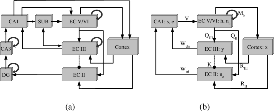
Figure 1. (a): Diagram of the main connections of HR. Arrows denote excitatory connections and solid circles denote mostly inhibitory connections. (b): Connections playing a role in the model. Roman letters denote the layers in the entorhinal cortex (EC),
$\mathbf{x}$: signal from cortex,
$\mathbf{y}$: whitened input at EC III,
$\mathbf{n_{z}}$: whitened novelty (or innovation) of the input at EC II,
$\mathbf{h}$: hidden model at EC deep layers,
$\mathbf{n}_{\mathbf{h}}$: innovation of the hidden model at EC deep layers,
$\mathbf{s}$: ICA output at CA1 during positive theta phase,
$\mathbf{e}$: ICA output at CA1 during negative theta phase,
$R_{II}$ and $R_{III}$: postrhinal to EC II and postrhinal to EC III efferents, respectively,
$Q_{II}$ and $Q_{III}$: EC deep layers to EC II and EC III connections, respectively,
$K$ inhibitory feedback from EC III to EC II.
$V$: CA1 to EC deep layer efferents,
$M_{h}$: recurrent collaterals at the deep layers of the EC,
$W_{tri}$ and $W_{dir}$: tri-synaptic and direct connections between EC superficial layers and the CA1 subfield, respectively.

Direction of information flow

First, there is a dominantly unidirectional ([Naber et al., 2001], but see [Shao and Dudek, 2005]), and parallel connection system among all parts: superficial layers of EC receive input from adjacent cortical regions and transmit the signals toward CA1 and the subiculum mediated by CA3. This transmission, however, is not a simple relay: it takes place in a tightly controlled way using two separate routes: the so-called tri-synaptic connection system (EC II–DG–CA3–CA1) and the direct route from EC III to CA1. As the exact nature of the input received by EC II and EC III is not known and we want to focus on the functioning within the HR, we assume that the superficial layers share the same cortical input. We also assume that differences in the activity of these layers stem from their differing intrinsic physiology (e.g. the ratio of interneurons that enables strong feedforward inhibition in EC II), anatomy (role of recurrent collaterals) and the received feedback (EC layers V/VI project back to both layers and EC III receives signals from the subiculum, too).

CA1 and the subiculum, which are considered to be the main output regions of the HR, project back to the deep layers of EC. In parallel with the subicular pathway, CA1 is linked to the deep layers directly as well. The parallel systems in part preserve topographical arrangement [Witter, 2006] but there exists a separation along the lateral to medial direction. The lateral and medial parts of the entorhinal cortex (LEC and MEC, respectively) receive input from different cortical areas and, in turn, project to non-overlapping portions of CA1 and the subiculum. In contrast, DG and CA3 receive convergent input from both LEC and MEC. An important functional consequence is that the fusion of spatial and non-spatial information may be strictly controlled within HR [Gigg, 2006, Witter and Moser, 2006].

The EC deep layers, which presumably also receive modulatory or control signals from different cortical areas, close the loop: they send mostly excitatory [van Haeften et al., 2003] feedback to the superficial layers.

Unique intra-regional interactions in each area

Although place cells can be found everywhere in DG, CA3 and CA1, their coding mechanism may be quite different, as the underlying connection systems have significantly distinct features. DG is unique for its temporally tunable connections [Henze et al., 2002]. CA3 has a dense collateral system which has a particular role in memory replay [Louie and Wilson, 2001, Foster and Wilson, 2006, Diba and Buzsáki, 2007, Csicsvari et al., 2007, O’Neill et al., 2008]. CA1, as a single exception in the whole circuitry, has no recurrent collaterals and the activity of the principal cells seems to be independent [Redish et al., 2001].

Temporal synchrony across and within different areas

In addition to the intricate anatomy, the physiology of the separate modules is also striking. The most prominent feature is the interplay between different forms of oscillatory activities, the synchronized membrane potential oscillation between the 4-10 Hz theta and the 40-100 Hz gamma frequency bands, [Bragin et al., 1995, Canolty et al., 2006], which have differential effects on the different modules. Several functional roles have already been assigned to these activity forms , such as the control of synchrony throughout the circuitry [Denham and Borisyuk, 2000] or the provision of an internal reference clock [Jefferys et al., 1996, Jensen et al., 1996].

The main generator of theta is thought to be in the septum (which is the only extra-hippocampal target of CA3), but layer EC II may also be able to initiate theta activity. The reciprocity between the subiculum and the HR via CA3 may suggest that HR has a sophisticated mechanism for self-regulating synchrony. In addition, EC II neurons are theta modulated and show phase precession, similarly to the place cells in the hippocampus [Hafting et al., 2005b].

EC III, which is very close to layer EC II, however, is phase locked to the main theta and can maintain persistent activity [Tahvildari et al., 2007]. Deep layers of the EC show peculiar functioning as well. In contrast to the superficial layers, EC V can generate input specific graded persistent activity in individual neurons [Egorov et al., 2002] which is generally considered the underlying neural mechanism of working memory [Goldman-Rakic, 1995]. Furthermore, the relative homogeneity of the CA1 response to changing inputs as compared to that seen in the deep EC may suggest [Frank et al., 2006] that active CA1 neurons are engaged in representing one environment, while deep EC may contain multiple subpopulations, some tied to CA1 output while others are more independent of CA1. Interestingly, separate modules or ‘cell islands’ can be found in EC II as well [Witter and Moser, 2006]. As a consequence, if deep layers can represent several likely models concerning the world, there should be a switching mechanism that can help select the one that best serves correct predictive coding. It is intriguing that layer III of the EC has been found to receive such switching signals [Tahvildari et al., 2007]. Last, but not least, signals carrying different aspects of spatial information, such as position, head-direction or speed, seem to interfere at several stages. While activity in CA3 and CA1 doesn’t show correlation with directional information, postsubicular head-direction cells directly innervate the deep layers of EC, which in turn send this information to the superficial layers. According to this scenario, grid cells in EC III show clear conjunctive correlation representing mixed information at the same time [Sargolini et al., 2006]. However, the activity of neurons in EC layer II is free of directional modulation.

4. Results

In the first part we formalize the proposed functions by providing a mathematical construction. In the resulting computational model the different functional modules are not yet anchored to the real system. Since this reverse-engineering approach (assignment of the functions precedes the description of the structure) is essentially ill-posed (offering several solutions), in the second part we attempt to map the modules onto the real neural system by taking into account the biological constraints collected in the previous section. Finally, simulations are presented in which the function of the model is demonstrated on inputs that can be related to signals received by the hippocampal region.

Results I: Formal description of the functional model

Let us assume the system’s goal is to form efficient representation of the sensory information which can be used for prediction. Efficiency refers to storage capacity (a small number of ‘factors’ should be used to reconstruct large number of possible inputs) and speed (the system should try out only a few combinations of the factors). Prediction is the ability to generate expected inputs. Let us begin with an abstract description of the observation of the external world (At this point we don’t model different sensory modalities. The input variable is simply a description of the external world). The sensory input $\mathbf{x}(t)$ to the system may be assumed to be a mixture of hidden source signals or causes:

(4.1) $$\mathbf{x}(t)=A\mathbf{s}(t),$$

where $A\in\mathbb{R}^{n\times n}$ is a mixing matrix, and $\mathbf{s}(t)\in\mathbb{R}^{n}$ are the sources to extract. Regarding our hypothesis (3), ICA is designed to solve a similar problem under the condition that the components of $\mathbf{s}$ are i.i.d., and statistically independent. However, the observed quantities may not be i.i.d.,

(4.2) $$\mathbf{s}(t+1)=F\mathbf{s}(t)+\mathbf{e}(t+1),$$

where $\mathbf{e}(t)$ is called the ‘driving noise’, ‘true source’, or ‘innovation’. The expression ‘driving noise’ refers to the fact that process $\mathbf{s}$ is maintained by the ‘true source’ $\mathbf{e}$: without this input, $\mathbf{s}(t)$ would decay. Due to the mixing effect of matrix $F$ which describes the deterministic part of the process, the components in $\mathbf{s}(t)$ are not independent anymore. Obviously one can envision more sophisticated systems. Nevertheless, for higher order processes or signals with echoes, the formalism can be brought to very similar forms [Lõrincz and Buzsáki, 2000, Szabó et al., 2007, Póczos et al., 2007]. As long as the components of the true source, $\mathbf{e}(t)$ can be considered independent, the efficient representation can again be achieved by extracting these components. If the dynamics are ‘weak’ in the sense that only weak temporal correlations are introduced by $F$, then we arrive at the original ICA problem. Because we are interested in the causes, i.e., in the driving noise, we need to learn both the autoregressive process ($F$) and the mixing process ($A$). This can be achieved [Lõrincz and Szabó, 2007] only if components of the true driving noises are independent. Under the normal (Gaussian) noise assumption the effects of these processes cannot be distinguished. We need to carry out some manipulations in order not to misguide ICA.

We make use of the identities

(4.3) $$\mathbf{x}(t+1)=A\mathbf{s}(t+1)=AF\mathbf{s}(t)+A\mathbf{e}(t+1))$$

to get

(4.4) $$\mathbf{x}(t+1)=M\mathbf{x}(t)+\mathbf{n}(t+1),$$

where $\mathbf{n}(t+1)\doteq A\mathbf{e}(t+1)$ and $M\doteq AFA^{-1}$ under the assumption that matrix $A$ can be inverted. Thus, both Eq. (4.2) and Eq. (4.4) have autoregressive forms. Due to the mixing effect of $A$ (Central Limit Theorem), the distribution of $A\mathbf{e}(t+1)$ is more Gaussian-like compared to the true sources. It implies that the standard solution of the Gaussian autoregressive processes can be applied as the first step to unfold the hidden processes.

Now let us suppose we have a tunable system and our task is to find the hidden process $\mathbf{s}$ and the driving source $\mathbf{e}$ using only the observation $\mathbf{x}(t)$. In what follows, we distinguish approximations of the true quantities by a small hat.

First, one can remove the autoregressive part by estimating matrix $\hat{M}$ through the minimization of the following cost function

(4.5) $$J(\hat{M})=\frac{1}{2}\sum_{t}|\mathbf{x}(t+1)-\hat{M}(t)\,\mathbf{x}(t)|^{2}.$$

for all available data pairs $(\mathbf{x}(t+1),\mathbf{x}(t))$. Then, we have a model that predicts the next expected input

(4.6) $$\mathbf{\hat{x}}(t+1)=\hat{M}(t)\mathbf{x}(t)$$

and we can estimate the innovation, i.e., the difference between the observed input and the expected input at time $t$:

(4.7) $$\mathbf{\hat{n}_{x}}(t)=\mathbf{x}(t)-\mathbf{\hat{x}}(t).$$

For Gaussian $\mathbf{\hat{n}_{x}}(t)$, the minimization of Eq. (4.5) leads to the following gradient rule:

(4.8) $$\Delta\hat{M}(t+1)=\alpha_{t}\,\big{(}\mathbf{x}(t+1)-\hat{M}(t)\,\mathbf{x}(t)\big{)}\mathbf{x}(t)^{\prime}=\alpha_{t}\,\mathbf{\hat{n}_{x}}(t+1)\mathbf{x}(t)^{\prime}$$

where prime ^′ denotes the transposed form for vectors and also for matrices, and $\alpha_{t}$ is the learning rate. If $\alpha_{t}$ diminishes according to some suitable schedule then $\hat{M}(t)$ converges to the real $M$ [Robbins and Monro, 1951]. In what follows, the learning rules will be written as

(4.9) $$\Delta\hat{M}(t+1)\propto\,\mathbf{\hat{n}_{x}}(t+1)\mathbf{x}(t)^{\prime}$$

where the sign ‘$\propto$’ denotes the Robbins-Monro schedule. Note, however, that if the world is changing then it is better to maintain adaptation forever.

So far we have exploited the Gaussianity property of the driving noise to learn the dynamical system. Now we can make use of the fact that upon convergence, the innovation term also converges to the mixed true sources of Eq. (4.1) ($\mathbf{n_{x}}(t)\mapsto A\mathbf{e}(t)$). In turn, simple separation of the innovation yields the demixing process $W$, which is the approximation of the inverse of the mixing matrix: $W=\hat{A}^{-1}$. Then $\mathbf{\hat{e}}(t)=W\mathbf{\hat{n}_{x}}(t)$ is the approximation of true sources, whereas $\mathbf{\hat{s}}(t)=W\mathbf{x}(t)$ approximates the hidden process.

One can approximate the autoregressive matrix $F$ using quantities $\mathbf{x}$, $\hat{M}$, and $\mathbf{\hat{e}}$. The goal of the approximation is to optimize prediction, that is, to minimize the following cost function:

(4.10) $$J(\hat{F})=\frac{1}{2}\sum_{t}|\mathbf{\hat{s}}(t+1)-\hat{F}(t)\,\mathbf{\hat{s}}(t)|^{2}.$$

As with matrix $M$, matrix $F$ can be learned through the following gradient rule:

(4.11) $$\Delta\hat{F}(t+1)\propto\,\big{(}\mathbf{\hat{s}}(t+1)-\hat{F}(t)\,\mathbf{\hat{s}}(t)\big{)}\mathbf{\hat{s}}(t)^{\prime}=\,\mathbf{\hat{e}}(t+1)\mathbf{\hat{s}}(t)^{\prime},$$

that is,

(4.12) $$\Delta\hat{F}(t+1)\propto\,\,W\mathbf{n_{x}}(t+1)(W\mathbf{x}(t))^{\prime}$$

This strategy has been detailed in [Lõrincz and Szabó, 2007].

Let us note that the gradient learning rules of Eqs. (4.8) and (4.11) may have plausible neural implementations as they are incremental and the change in one synapse does not depend on the change in all the other synapses. If this latter condition is met, then we say that learning is Hebbian, or alternatively, the learning rule is ‘local’.

As signals should be separated and — as was argued before — separation can be facilitated if whitening takes place first, a decorrelation stage might be introduced. According to [Çardoso and Laheld, 1996], signals $\mathbf{y}=P_{\mathbf{y}}\mathbf{x}$ become decorrelated if

(4.13) $$\Delta P_{\mathbf{y}}(t+1)^{\prime}\propto P_{\mathbf{y}}(t)^{\prime}(I-\mathbf{y}(t)\mathbf{y}(t)^{\prime})$$

for all times $t=1,2,\ldots$ and under suitable conditions. Note that here, in Eq. (4.13), and in similar equations later, the learning rule contains the transposed form of matrix $P_{\mathbf{y}}$ and thus dimension reduction ($\dim(\mathbf{y})\leq\dim(\mathbf{x})$) is possible. Intuitively this serial update algorithm pushes the covariance matrix of $\mathbf{y}(t)$ ($E(\mathbf{y\,y}^{\prime})$, where $E(.)$ denotes expectation) to become identity. Let us remark that there are many artificial neuronal implementations of such algorithms [Foldiak, 1990, Hyvärinen and Oja., 1998, Linsker, 1999, Basalyga and Rattray, 2003].

For the very same reason, innovation $\mathbf{n_{x}}(t)$ should also be decorrelated. The linear transformation $\mathbf{n_{z}}=P_{\mathbf{n_{z}}}\mathbf{n_{x}}(t)$ of innovation $\mathbf{n_{x}}(t)$ becomes white if tuning of $P_{\mathbf{n_{z}}}$ is as follows:

(4.14) $$\Delta P_{\mathbf{n_{z}}}(t+1)^{\prime}\propto P_{\mathbf{n_{z}}}^{\prime}(t)(I-\mathbf{n_{z}}(t)\mathbf{n_{z}}(t)^{\prime})$$

at time $t$.

Statistically independent sources from $\mathbf{n_{z}}$ can be extracted via a nonlinear modification [Çardoso and Laheld, 1996] of update rule Eq. (4.14). There are many variants for this non-linear learning rule and we provide the simplest of these here:

(4.15) $$\Delta W_{\mathbf{n_{z}}}(t+1)^{\prime}\propto W_{\mathbf{n_{z}}}(t)^{\prime}(I-\mathbf{\hat{e}}(t)\,f(\mathbf{\hat{e}}(t))^{\prime}).$$

Here, $f(\cdot)$ is an (almost) arbitrary component-wise nonlinear function. Upon convergence, the components of $\mathbf{\hat{e}}(t)=W_{\mathbf{n_{z}}}\mathbf{n_{z}}(t)$ approximate the components of the independent source $\mathbf{e}(t)$ apart from an arbitrary permutation in the order of the components, their scale and sign. Interestingly, spike timing dependent plasticity has been suggested to realize this non-linear learning rule [Bell and Parra, 2005].

The learning equations of the whitening and separation processes have several implications concerning possible mappings.

Two stages:

Removal of the temporal correlations precedes the extraction of the independent factors.

Two channels:

According to Eq. (4.11), the process of learning the predictive system requires concurrent access to the input and the innovation. These variables may be stored separately and conveyed to the predictive layer via separate channels.

Identical separation:

It can be seen from Eq. (4.12) that both $\mathbf{\hat{e}}(t)$ and $\mathbf{\hat{s}}(t)$ are demixed by the same matrix, so they should be processed in the same demixing channel (violating the conjecture above) or there should be a mechanism that can compensate for the differences (e.g., sign and permutation of the components) in the linear transformations in two channels for proper demixing.

Results II: Functional mapping of the model

Since both the computational considerations and the anatomical findings are quite complex, we need to introduce some simplifications:

Rate coding:

How information is actually transmitted by the neurons is neglected. The key issue is that once the particular form is given, the function of the system can be analyzed as an information processing system. (On the controversies concerning the potential forms of information processing, however, see e.g.  [Reyes, 2003, Masuda and Aihara, 2007].) Our system description becomes simpler if we use analog values, which corresponds to the concept of rate coding as opposed to spike based temporal coding. The supposed low-pass filtering effect of the theta oscillation also suggests that for some functions fine scale temporal precision might be neglected.

Laminar homogeneity:

We neglect the complexity and richness at the cellular level and consider neurons as computational units. The computations may change from layer to layer, but within a layer the nature of the computation is the same for all neurons. This corresponds to the terminology of standard artificial neural networks.

Apparent linearity:

Although strong nonlinearities are present everywhere, from the subcellular level to the network level, there are nonetheless many cases in which the overall response of the system is approximately linear, see, e.g.,  [Linsker, 1999], [Hsu et al., 2004] and [Escabi et al., 2005] and the cited references. The complex contrast normalization mechanisms in visual sensory processing may constitute a specific example [Finn et al., 2007].

>From now on, matrices denote synaptic weights (connection strength) between layers and vector denotes the activity at a given layer. We shall slightly abuse notation and will discard the hats from our equations, as all learned quantities are approximations.

Figure 1 may help to understand the modular structure of our model and its relation to the hippocampal region. While the left panel depicts the gross anatomy of the areas, including the different connection systems, the right panel of Fig. 1 shows the simplified architecture and the functional correspondences.

The following areas of the hippocampal regions are considered in the functional mapping: deep layers of the medial entorhinal cortex (denoted by EC V/VI), superficial layers (EC II and EC III) and subfield CA1 of the hippocampus. The tri-synaptic path (denoted as $W_{tri}$ on Fig. 1) involving the Dentate Gyrus (DG) and CA3 will be collapsed into an integrated transformation. The potential role of the DG, CA3 as well as the Subiculum (SUB) will be discussed in the last section. For simplicity, all areas and subfields will be referred to as ‘layers’.

As all computations described above require statistical characterization of input ensembles, sampling and processing of the sensory input and incremental tuning (learning) are also necessary. Input processing and learning, i.e., fine tuning of the synaptic weights that actually filter the information, are discussed separately.

Characterization of the input to the hippocampal region

Let $\mathbf{x}(t)\in\mathbb{R}^{n}$ denote the analog valued postrhinal input to the entorhinal cortex at discrete time $t$ where $n$ is the dimension of the input. In this model, we limit ourselves to square problems, which is to say that $n$ may be considered as both the number of postrhinal neurons and the number of entorhinal neurons of the targeted layer. Let us also assume that the input follows the dynamics described above. The postrhinal input enters the circuitry at the superficial layers of EC through two parallel connection systems $R_{II}\in\mathbb{R}^{n\times n}$ and $R_{III}\in\mathbb{R}^{n\times n}$, so, we assume that the number of principal cells in each superficial layer is equal and is also $n$. These connection systems may only transmit cortical input to HR, so their tuning is omitted: admitting the lack of knowledge concerning the exact nature of the parallel postrhinal inputs, we may suppose that $R_{II}=R_{III}=I$, where $I\in\mathbb{R}^{n\times n}$ denotes the $n\times n$ identity matrix. When the process of learning the matrices is considered, a temporal index is shown in most cases. For better readability the time index is dropped for non-tunable matrices and in the dynamical equations.

>From EC II/III the signals are sent to the hippocampus through the direct, i.e., EC III$\,\rightarrow\,$CA1, and the indirect,tri-synaptic i.e., EC II$\,\rightarrow\,$CA1 pathways (denoted by subscripts ‘dir’ and ‘tri’ on the right hand side of Fig. 1, respectively).

Detailed correspondence between the functional model and the neural layers of the HR

The formal description has some direct consequences concerning the potential roles of the different layers of the HR. First, it is obvious that innovation (that is the comparison of the predicted and actual inputs) can only be stored in a layer that not only receives the input, but is also the target of inhibitory feedback. Due to its widespread inhibitory network, EC II is assigned to hold the innovation. The activity at EC II is as follows:

(4.16) $$\mathbf{n_{z}}(t+1)=R_{II}\mathbf{x}(t+1)+Q_{II}\mathbf{h}(t)-K\mathbf{y}(t),$$

where $\mathbf{y}(t)$ and $\mathbf{h}(t)$ denote the activity at EC III and EC V/VI, respectively. (Roman subscripts of the connection matrices denote the number of targeted layers.) Connections from EC III to EC II, denoted by $K$, are assumed to be mostly inhibitory. The reason for this assumption is that the vast majority of the deep to superficial connections are excitatory and mostly target principal cells in EC II [van Haeften et al., 2003] and the cortical inputs are also of excitatory nature. In turn, $K$ is the candidate connection system that effectively targets the inhibitory network of EC II. Here, the role of $Q_{II}$ is to whiten the innovation, whereas the role of $K$ is to ensure that the emerging activity pattern is indeed proportional to the required innovation.

Equation (4.16) and the connectivity of the HR implies that $\mathbf{y}(t)$ should be proportional to the input and is made of two terms from bottom-up and top-down contributions. The activity of EC III is thus the following:

(4.17) $$\mathbf{y}(t)=R_{III}\mathbf{x}(t)+Q_{III}\mathbf{h}(t),$$

where $Q_{III}$ — in accordance with the redundancy reduction principle — is assumed to decorrelate the activity at the targeted layer, EC III. However, decorrelation of quantity $\mathbf{y}(t)$ may influence (distort) the innovation in EC II. This raises some doubts, because quantity $\mathbf{n_{z}}(t+1)$ might be contaminated by predictable components, or its whiteness might be spoiled. In turn, tuning of matrix $K$ should somehow counteract both problems under the constraint that learning is Hebbian. The solution to this threefold problem is an emerging property in our model.

As was noted earlier, CA1 has a central location since it is targeted by both layers EC III and EC II via $W_{dir}(t)\in R^{n\times n}$ and $W_{tri}(t)\in R^{n\times n}$, respectively:

$$\mathbf{s}(t)=W_{dir}(t)\mathbf{y}(t),$$

where $\mathbf{s}(t)\in R^{n}$ denotes the activity of CA1, if its driving input is projected from EC III and

(4.18) $$\mathbf{e}(t)=W_{tri}(t)\mathbf{n_{y}}(t),$$

where $\mathbf{e}(t)\in R^{n}$ denotes the activity of CA1, if its driving input is projected from EC II. Following the proposal of [Lõrincz, 1998, Lõrincz and Buzsáki, 2000] and supported by the experimental findings of  [Redish et al., 2001], independent components should be expressed in CA1. In turn, we believe transformations $W_{dir}(t)$ and $W_{tri}(t)$ realize the actual signal separation and provide approximate independent components. We note that according to Eq. (4.2) $\mathbf{e}(t)$ should be equal to the innovation of $\mathbf{s}(t)$. However, unlike in the superficial layers, there are no recurrent collaterals in CA1. This means that for properly tuned $Q_{II}$, $Q_{III}$ and $K$, the two bottom-up transformations, i.e., $W_{tri}$ and $W_{dir}$ should become effectively identical in the absence of recurrent collaterals.

CA1 signals may leave the loop through the subiculum or they may be sent back to the deep layers of EC via the connection system denoted by $V\in R^{n\times n}$. (On the intriguing properties of $V$ (not modeled here), see [Naber et al., 2001]).

In line with [Lõrincz et al., 2002], a central function of the deep layers of EC may be pattern completion. However, as was already noted, forcing independence does not support pattern completion. It is also known ?that activity patterns of the deep layers of EC are not in fact independent [Sargolini et al., 2006]. This implies that ‘remixing’ of the components is advantageous. Of the many possibilities, whitening seems the most straightforward transformation, as it does not increase the number of transformations within the EC-HC circuitry. The resulting patterns may show higher-order correlations supporting the task of pattern completion. Since the internal predictive system is based on the intensive use of recurrent connections, only CA3 and EC V/VI may be considered. If our assumption about the roles of the superficial layers are valid, then EC V/VI should realize the predictive system since CA3 is not supposed to receive significant input from EC III.

Consequently, the activity at EC V/VI can be written as:

(4.19) $$\mathbf{h}(t+1)=M_{h}\mathbf{h}(t)+\mathbf{n_{\mathbf{h}}}(t),$$

where predictive system $M_{h}$ can propagate activity $\mathbf{h}(t)$ in time, $\mathbf{h}(t)=V\mathbf{s}(t)$ and $\mathbf{n_{\mathbf{h}}}(t)=V\mathbf{e}(t)$. In addition to conveying information from CA1, V is responsible for the decorrelation of the activity patterns. $M_{\mathbf{h}}$ is an approximation of the dynamical model underlying the observations (see Eq. (4.2)). The queuing of the arrival of the two different inputs ($\mathbf{s}(t)$ and $\mathbf{e}(t)$) requires a mechanism that can maintain activity long enough to enable integration. Experimental findings on gradually modifiable persistent activity in EC V [Egorov et al., 2002] may support this proposal.

At last, the deep layers project back to EC II and EC III via $Q_{II}$ and $Q_{III}$, respectively.

Learning processes

For different reasons, 3 connection systems are assumed to decorrelate the activity of their targeted layer: $Q_{II}$, $Q_{III}$, and $V$. Their tuning follows the form given in Eqs. (4.13) or (4.14). For example, learning of $Q_{II}$ can be given as:

(4.20) $$\Delta Q_{II}(t+1)^{\prime}\propto Q_{II}^{\prime}(t)(I-\mathbf{n_{z}}(t)\mathbf{n_{z}}(t)^{\prime})$$

where $\mathbf{n_{y}}(t)$ is the emerging activity of the targeted layer, EC II.

To arrive at the right form of innovation, connections between EC III and EC II need to be tuned. The learning rule of $K(t)$ is supposed to satisfy a Hebbian form, similar to Eq. (4.9)

(4.21) $$\Delta K(t+1)\propto\,\mathbf{n_{z}}(t+1)\mathbf{y}(t)^{\prime}.$$

This is the perfect learning rule, because it minimizes cost function

(4.22) $$J(K)=\frac{1}{2}\sum_{t}\big{|}R_{II}\mathbf{x}(t+1)+Q_{II}\mathbf{h}(t)-K\mathbf{y}(t)\big{|}^{2}=\frac{1}{2}\sum_{t}\big{|}\mathbf{n_{z}}(t+1)\big{|}^{2}.$$

which is the Euclidean norm of $\mathbf{n_{z}}$. In this expression each term is a linear transform of $\mathbf{x}$ with different time lags. The result of the learning rule is that, apart from an arbitrary linear transformation,

$$K\mathbf{y}(t)=Q_{II}\mathbf{h}(t)+R_{II}\mathbf{x}(t),$$

is satisfied in all instances. This is the net result, i.e., $\mathbf{n_{z}}(t)$ is indeed a linear transform of innovation $\mathbf{n_{x}}(t)$. Quantity $\mathbf{n_{z}}(t)$ will be white given the learning rule for $Q_{II}$ detailed in Eq. 4.20. In sum, learning rule Eq. 4.21 is Hebbian and adjusts the inhibitory contribution until $\mathbf{n_{z}}(t)$ becomes a linear transformation of the innovation, subject to the constraint, that both $\mathbf{y}(t)$ and $\mathbf{n_{z}}(t)$ are white.

Separation takes place in both the direct and the indirect pathways, so $W_{dir}$ and $W_{tri}$ should undergo tuning similar to Eq. (4.15). At this point some remarks are in order. We expect to have two separate channels, one for the input and one for the innovation, which can basically reverse the mixing effect of the very same mixing process (see Eq. (4.1)). We have also seen that both separation processes would probably end up creating approximately independent components in the same layer (CA1). First, it is necessary to ensure that learning in the two separation pathways converges to approximately the same solution. Second, it is necessary to schedule the activity at CA1 to avoid interference between the patterns corresponding to the independent components of the input or the innovation. Regarding the interaction between $W_{dir}$ and $W_{tri}$, it is intriguing that while the original problem of ICA (that is when the mixing process and the components are unknown) is truly unsupervised, by constraining the outputs of the tunable matrix to some prescribed outputs the learning algorithm becomes supervised. Thus, the two matrices may become identical if one channel dominates (supervises) the other. Physiological considerations seem to suggest a possible mechanism.

Regarding separation, in the beginning the faster direct pathway may supervise the indirect one by providing approximately independent components in CA1. We note that there is a temporal coordination between the firing of the neurons that send information through the direct and the indirect paths [Dragoi and Buzsáki, 2006]. It is also possible that supervising signals may reach CA1 at one phase of the theta oscillations, while the signals from the tri-synaptic pathway may reach CA1 at the other phase. Another argument is that although place fields in CA1 begin to stabilize early (compared to the place fields in CA3) and even without input from the tri-synaptic route, full stabilization takes much longer. We suggest that the two routes work together. The early stabilization results in approximate independent components if the signal from EC III is contaminated by large temporal correlations. The task of the indirect route may be to diminish this kind of temporal dependence and to proceed with the separation of the sources, but this is a slower process.

Following our hypothesis, tuning of $W_{dir}(t)$ and $W_{tri}(t)$ may assume two different forms during the course of learning:

(4.23) $$\Delta W_{dir/tri}(t+1)^{\prime} \propto W_{dir/tri}(t)^{\prime}(I-\mathbf{s}(t)\,f(\mathbf{s}(t))^{\prime})$$

(4.24) $$\Delta W_{dir/tri}(t+1)^{\prime} \propto W_{dir/tri}(t)^{\prime}(I-\mathbf{e}(t)\,f(\mathbf{e}(t))^{\prime}).$$

where $f(\cdot)$ is an (almost) arbitrary component-wise nonlinear function.

In the formal model we have seen that all these transformations are required to provide the right information for the internal predictive model. However, this model also needs tuning in order to match the observed signals.

The approximation of predictive matrix $M_{\mathbf{h}}$ – as with all predictive matrices in the model – can be written as follows:

(4.25) $$\Delta M_{\mathbf{h}}(t+1)\propto\,\mathbf{n}_{\mathbf{h}}(t+1)\mathbf{h}(t)^{\prime}$$

This rule trains matrix $M_{\mathbf{h}}$ to optimize prediction in with? Euclidean norm norms?. Due to the scheduled arrival, we need to suppose that the time window is broad enough to enable interaction of the transformed input signal and the innovation. As we see, training is Hebbian, but a detailed mechanism that would actually be able to carry on this tuning is missing. Nevertheless, we conjecture that the double loops of the direct and indirect pathways have a fundamental role in tunneling the right information at the right time. It is worth noting that this assumption is also supported by the experimental finding that activity in CA3 under one theta oscillation (50-80 ms) may correspond to 1 second of the external sensory flow. Unfortunately, available experimental data is not sufficient to better model this interplay.

In summary, if all transformations are optimally tuned, then (1), temporal correlations $F$ are learnt and represented in the internal model through matrix $M_{\mathbf{h}}$, (2), the hidden processes $\mathbf{h}$ can be estimated by the learnt model and (3), the true independent causes $\mathbf{e}$ can also be revealed. Note that two main goals are achieved; the independent causes ($\mathbf{e}$) are revealed up to an arbitrary permutation, scale and sign, and the predictive matrix $F$ is learnt up to a linear transformation.

In the next section we turn back to the original problem of the emergence of particular spatial activity at different parts of the HR. In the simulations the transformations assigned to different parts of the loop are implemented and applied on structured high dimensional inputs containing spatial information. The goal is to study whether the emergent activity at the different modules corresponding to e.g. CA1 and ECII/ECIII resembles that found experimentally.

Results III: Simulations

We present a series of simulations with inputs of increasing complexity. The more realistic the inputs, the more complex the computations that are required to extract spatial information. In doing so, the role of different modules can be highlighted.

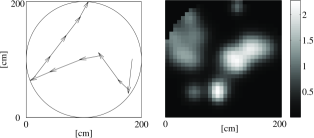
Figure 2. (a): Circular maze, diameter: 2m, with a short sample trajectory. Step size varies between 11 and 55 cm. (b): Sample input to the loop in the form of an activity map within the maze (see, Eq. (4.27) for details). Activity map is shown in arbitrary units.

In our sample simulations a virtual rat has explored a 2 m wide, open-field circular maze. Similar results were reached using a square maze. The path has been generated as follows: the rat runs on a linear path at a constant speed and makes a small random turn at each step with a given chance. It also makes a random turn if it ‘senses’ that it may collide with the wall. Input sampling has been fixed to 55 cm. The length of this random trajectory and input sampling were chosen to get a fair coverage of the full area of the maze with a reasonable number of samples. The maze and a sample trajectory is shown in Fig. 2. Inputs corresponding to turns may only be interpreted by higher order autoregressive processes for which the order would be about the average number of steps in a single direction. As the implemented internal model assumes first order processes (see the comment at Eq. (4.2)), such inputs have been excluded. We shall come back to this point in Section 5.

The most restrictive approximation in our simulations is that the input contains information about the local cues only, no distal information is included. One might think that the input is a mixture of smells that differs from point to point. This local nature implies that parametric maze distortions can not be modeled in this framework. On the other hand, this simplification excluded any artifact that would result from arbitrary modeling of low-level sensory processing. Instead, we simply mimicked postrhinal (‘parahippocampal’ in primates)  [Burwell and Hafeman, 2003] inputs. In contrast to perirhinal input  [Eacott and Gaffan, 2005], postrhinal input is assumed to reflect changes of spatial properties or directly carry spatial information (albeit in weak correlations,  [Fyhn et al., 2004]). Such spatial dependence of the postrhinal activity was approximated by first creating $n$ Gaussian patches with each Gaussian having a maximum amplitude of 1:

(4.26) $$g_{i}(\mathbf{p})=\exp\left(-\frac{(\mathbf{p}-\mathbf{c}_{i})^{2}}{\sigma_{i}^{2}}\right),$$

where $\mathbf{p}\in\mathbb{R}^{2}$ denotes the coordinate vector of the rat, $\mathbf{c}_{i}\in\mathbb{R}^{2}$ is the coordinate vector of the center of the $i^{th}$ Gaussian, and $i\in\{1,\ldots,1000\}$. Centers $\mathbf{c}_{i}$ were drawn from the uniform distribution over the full maze while $\sigma_{i}$ were uniformly drawn from the range [20 cm, 40 cm].

Input $\mathbf{x}$ was created by using a random, binary mixing matrix $G\in[0,1]^{1000\times 1000}$ over the set of the Gaussians:

(4.27) $$\mathbf{x}(t)=G\,\mathbf{g}(\mathbf{p}(t)),$$

where $\mathbf{p}(t)$ denotes the coordinates of the rat in the maze at time $t$ and the $i^{th}$ component of vector $\mathbf{g}\in R^{1000}$ is $g_{i}(\mathbf{p}(t))$ at time $t$. Each row of matrix $G$ contains 20 positive non-zero elements on average. The resulting activity map for a single component of $\mathbf{x}(t)\in R^{1000}$, i.e., for one of our ‘sensors’ is shown in Fig. 2(b).

In simulation #1 the input to the model was exactly as defined in  (4.27).

In simulation #2 50 more units were added, so the dimension of the input, $\mathbf{x}(t)$ was 1050. The new units ‘sensed’ directions and had no spatial dependence. The direction sensitivity has been defined as:

(4.28) $$x_{i}=f_{i}(\phi)=\max(0,\cos(\phi-\phi_{i})),$$

for $i\in\{1001,\ldots 1050\}$, where $\phi$ denotes the direction between the last and the current positions and $\phi_{i}$ denotes the direction for which the $i^{th}$ component ($1000<i\leq 1050$) is the most sensitive. This particular choice results in broadly tuned ($\sim\pi/2$) directional activities.

In simulation #3, instead of mixing the units that carry different information, we used 1000 conjunctive inputs that carried spatial and directional information:

(4.29) $$\mathbf{x}_{i}(t)=f_{i}(\phi(t))\,\left[G\,\mathbf{g}(x(t),y(t))\right]_{i}$$

where $\phi(t)$ is the direction of the rat at time $t$.

Last, in simulation #4, we used low-pass filtered versions of the inputs of simulation #3:

(4.30) $$\mathbf{x}^{(tc)}(t+1)=(1-\alpha)\mathbf{x}^{(tc)}(t)+\alpha\,\mathbf{x}(t+1)$$

where superscript ‘$tc$’ stands for ‘temporally convolved’. This is essentially the simplest autoregressive process regarding Eq. (4.2).

Spatial analysis

As opposed to real spiking data, linear transformations may give rise to negative signals. In turn, the correspondence between the unit activity values after each transformation and the neurons’ responses is not straightforward. In order to generate the activity maps of the input units, first we discretized the space (the resolution was $30$ so a bin is $6.67\,$cm$\times 6.67\,$cm, which is comparable to  [Hafting et al., 2005a]), and for each bin we summed up the activity measured in those steps that ended in the given bin. This spatial averaging smoothes out the artifacts caused by unattended spots. The activity after, e.g., decorrelation may assume negative values, so the data were half-wave rectified (clipped) and scaled to range $[0,1]$.

ICA is invariant for the change of sign  [Jutten and Herault, 1991]. In turn, the sign of an activity map has been defined by the average sign of the first 10 bins with the highest absolute value. That is, if more than 5 units were negative, we simply flipped the sign of the map. The resulting maps were then half-wave rectified. We also computed the 2 dimensional normalized autocorrelation for each activity map.

The spatial analysis of the peak activity regions for the autocorrelation image has been done by fitting a grid on the locally maximal points using Delaunay-triangulation  [Markus et al., 1995, Takács and Lőrincz, 2007]. Border vertices and nodes have been excluded from the analysis. Vertices are considered as internal if they belong to two triangles and nodes are internal if they only connect to other nodes through internal vertices. To characterize the regularity of the resulting grids, we calculated the vertex length and the angle distribution. Discretization, however, defines a lower bound of the edge length, which is about 2 bins, that is $\sim 13.34\,cm$. Because the mean angle in Delaunay-triangulation is obviously 60 degrees, the spread around this value (that is the standard deviation, or std for short) can be used to quantify regularity. The distribution of the mean vertex lengths and the distribution of the std of the angle values for the whole population have been used to compare the spatial characteristics of the input set and the set of the transformed signals.

For simulations #2, #3, and #4, direction sensitivity has also been analyzed. To show the spatial distribution of the direction sensitivity, we discretized the activity maps into $10\times 10$ bins and in each bin we collected those steps that ended in that bin. Their direction, weighted by the response value at the end point, was then added up. The resulting directed activity values can be visualized in a ‘direction-field’ plot. In order to characterize the spatial heterogeneity of the directional selectivity, the directed values may also be grouped according to their direction and these lumped sum values will be presented on a polar plot. These analysis serve to characterize the strength of spatial heterogeneity in direction selectivity.

Simulation #1: direction-independent input

Standard PCA reduced the dimension of the decorrelated input from 1000 to 852 as the remaining eigenvalues were below the level of numerical precision. The first 127 dimensions carried 95% of the total variance and the first 203 carried 99%. The resulting activity maps are comparable to the firing rate maps shown in  [Hafting et al., 2005a].

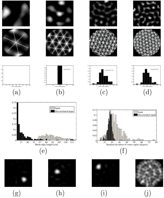
Figure 3. Simulation #1: position dependent input. (a-d): each column shows the output of different decorrelating units (PCA). First row: half-wave rectified and scaled activity maps (0: black, 1: white). Second row: 2D autocorrelation function of the activity maps and the fitted grids. Third row: vertex angle histogram for the fitted grids. (e-f): cumulative statistics over all grids. (e): histogram of the mean edge length of the grids for the input set and the PCA units. (f): histogram of the standard deviation of the vertex angles for the input set and the PCA units. (g-i): sign corrected activity maps of three separating (ICA) units. Response is localized. (j): superimposed map of all ICA units demonstrating that the localized units cover the full maze.

Subfigures 3 (a-d) show the spatial activity of 4 sample units. The first row depicts the clipped activity maps. We put the 2D autocorrelation functions of the activity maps and the superimposed grids into the second row. Note that the peak-to-peak distance varies over a broad range. The third row represents the vertex angle distribution of the corresponding grids. Narrower distribution means more uniform vertices and thus a more symmetric grid. Subfigures 3(e) and (f) show cumulative statistics concerning the grids. Only the grids of the first 220 largest eigenvalues have been used in these analyses as the rest are mostly noise. Subfigure 3(e) compares the distribution of the mean vertex length of the fitted grids for the input activity maps and the activity maps of the decorrelated inputs. Subfigure 3(f) compares the distribution of the standard deviation of the vertex angles of the fitted grids. Again, for hexagonal-like grids, the smaller the standard deviation, the larger the regularity. While the experimental data available to us is not sufficient for comparisons, we can safely claim that these grids do cover a range similar to those of [Hafting et al., 2005a]. These diagrams unambiguously show that the ‘gridness’ of activity has increased significantly due to the decorrelation step. Since the creation of the input is essentially equal to a random mixture, the effect we show here is not an artifact.

For the sake of completeness, the effect of separation is also shown. It was demonstrated in [Takács and Lőrincz, 2007, Franzius et al., 2007] that inputs with grid-like spatial activity patterns can be transformed into more localized ‘place cell’-like activity patterns by imposing independence or sparseness on the components of activity. As decorrelation in our simulations already yields grid activity, separation (into independent components) naturally resulted in unimodal place-cell like activity maps. Subfigures 3(g-i) show three sample units and subfigure 3(j) depicts the superposition of activity maps of 60 independent units. The resulting coverage may be interpreted as coarse grain disretization of a low-dimensional space (in our particular case, the relevant dimension is 2).

Simulation #2: Mixture of direction-independent and position-independent inputs

After decorrelation most grid structures were almost identical to those of simulation #1 (Fig. 4(a-d)). However, many units also showed a certain degree of direction selectivity, too. Clearly this ensemble of units with different dependencies shows an apparent conjunctive representation of position and direction. Similar representation was found in dMEC III-V  [Sargolini et al., 2006]. However, separation after decorrelation unambiguously shows (Fig. 4(e-g)) that there are now 2 relevant subspaces: direction and position. While most cells showed place-cell like activity (e.g. Fig. 4(e)), the rest of the units showed no spatial dependence: they were selective only for direction. For each subspace, separation essentially resulted in a coarse grain discretization. We emphasize that the decoupling of the directional information did not require any predictive mechanism in this case. It can be explained by the fact that a subgroup of the original inputs contained explicit directional information so their activity statistics are obviously different from the other units in the linear mixture.

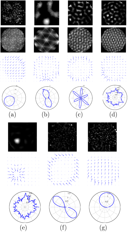
Figure 4. Simulation #2: mixture of purely position and purely direction selective inputs. (a-d): columns correspond to the output of different decorrelating units (PCA). First row: half-wave rectified and scaled activity maps. Second row: 2D autocorrelation function of the activity map and the fitted grid. Third row: spatial distribution of the direction selectivity is shown on a square grid of size 10x10. Fourth row: overall direction selectivity in the form of a polar plot. (e-g): columns correspond to the output of different separating units (ICA). First row: sign flipped, half-wave rectified activity maps. Second row: spatial distribution of the direction selectivity is shown on a square grid of size 10x10. Third row: overall direction selectivity in the form of a polar plot.

Simulation #3: Position and direction dependent inputs

For true conjunctive inputs (i.e. all input units show both position and direction selectivity), two changes can be seen in the activity maps of the decorrelating units (Fig. 5)(a-d). First, all units inherited the conjunctive property showing some direction selectivity on top of the grid-like spacing. Second, regularity and symmetry properties degraded in both subspaces compared to those of Fig. 4(a-d). The output of the separating units (ICA), in contrast to Simulation #2, now all showed significant direction selectivity as well (Fig. 5)(e-f). It implies that the ICA units are again local, but now in 3 dimensions: ICA cells basically discretize the Cartesian product of the 2 dimensional maze and the 1 dimensional space of directions.

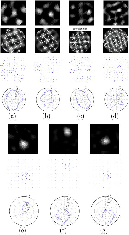
Figure 5. Simulation #3: position and direction selective inputs. (a-d): columns correspond to the output of different decorrelating units (PCA). First row: half-wave rectified and scaled activity maps. Second row: 2D autocorrelation function of the activity map and the fitted grid. Third row: spatial distribution of the direction selectivity is shown on a square grid of size 10x10. Fourth row: overall direction selectivity in the form of a polar plot. (e-g): columns correspond to the output of different separating units (ICA). Fifth row: sign flipped, half-wave rectified activity maps. Sixth row: spatial distribution of the direction selectivity is shown on a square grid of size 10x10. Seventh row: overall direction selectivity in the form of a polar plot.

According to our hypothesis, the internal model realized in the deep layers of the entorhinal cortex is responsible for restoring the decoupling between predictable (i.e., direction selective) and nonpredictable information. In turn, we expect to see weaker direction selectivity if the predictive model is also part of the computations (the circuitry now works on the difference (innovation) between the input and the expectation of the system’s internal model, see Eq. (4.16)). If the internal model is correctly tuned, then directional sensitivity should disappear from the innovation, resulting in clear hexagonal spacing again. Furthermore, we should see a diminished direction selectivity in place cell activity as well. Indeed, the directional sensitivity of the innovation of the decorrelated inputs decreased considerably, although the hexagonal structure of Fig. 5 did not improve significantly (results are not shown). In addition, separation of the innovation yielded local activity with diminished direction selectivity as predicted (Fig. 6).

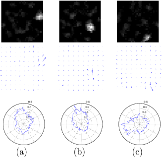
Figure 6. Innovation on the decorrelated conjunctive inputs. (a-c): columns correspond to the output of different separating (ICA) units. First row: half-wave rectified activity maps. Second row: spatial distribution of the direction selectivity is shown on a square grid of size 10x10. Third row: overall direction selectivity in the form of a polar plot.

Simulation #4: Temporally convolved position and direction dependent inputs

As we noted earlier, theta oscillation may be responsible for time compression in the HR, which – from the computational point of view – corresponds to temporally convolved inputs. The resulting moving average would probably highlight those factors that change less abruptly. In our case, apart from the turns taken in order to avoid collisions, directional information is either constant or varies slowly over a longer time interval. In turn, we expect to see that separation on the temporally convolved inputs collected during linear motion would yield stronger direction sensitivity with larger and less precise place fields (Fig. 7), similar to those found in the different areas of the subicular complex  [Sharp, 1996]. Direction selectivity has a much finer scale than the half-rectified cosine dependence used for the inputs.

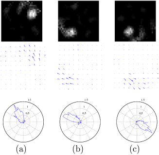
Figure 7. Separation on temporally convolved, position and direction dependent inputs. (a-c): each column corresponds to different ICA output units. First row: sign flipped and half-wave rectified activity maps. Second row: spatial distribution of the direction selectivity is shown on a square grid of size 10x10. Third row: overall direction selectivity in the form of a polar plot.

5. Discussion

In this last section, we analyze the simulation results and re-evaluate the functional mapping of our computational model. These considerations then lead to some predictions about the HR. We conclude with a discussion of a few issues still left unresolved and identify possible further improvements.

Interpretation of the simulation results

Although our model construct is based on general ideas about efficient representation of sensory events, when applied to spatially anchored inputs it has shown some intriguing properties that can directly correspond to experimental data.

The model correspondences have already been supported by the first simulation in that grid-like activity has appeared in exactly those modules the neural substrates of which were reported to present this particular activity. Once grid-like activity is present, forcing independence results in localized activity, as was shown for example, in [Franzius et al., 2007]. What is more interesting, though, is that reciprocity (i.e., place cells are needed to get stable grid cells) can also be explained by the loopy structure of our model. Another observation is that the weak overlap among the resulting place fields can be considered as discretization of the space. Similarly to what was found first in [Lõrincz et al., 2001], this is what ICA seems to do if there is a small dimensional space behind the high dimensional inputs.

In Simulation #2, directional information was introduced by mixing output of position dependent and purely direction dependent units. Let us remark here that no such labeling as position or direction was given in the model. The proposed algorithms simply extract statistical properties of the input ensemble. This simulation yielded two interesting results. The first one is that grid cells now show conjunctive behavior as well: in addition to pure position dependence, many units appear to depend on both space and direction. The other result that independent components now either show spatially localized activity with no direction selectivity or demonstrate clear direction-selectivity without any particular position dependence is a consequence of our input preparation, because we mixed two signals with different statistical properties and ICA separated them. Now, ICA discretizes two distinct subspaces separately; the space of position and the directional space. This is not unlike how information flow is supposed to take place between CA1 and subiculum. It is, however, interesting that despite the significant temporal correlation carried by directional information, separation alone (i.e. without activation of the predictive system) was able to decouple these different pieces of information. These observations also show the robustness of the ICA algorithm.

In Simulation #3, all input units had position and direction dependence (sampled from the product space of positional and directional information). In this case decorrelation and extraction of the components yielded distorted, less regular grid activity and all independent components showed directional dependence as well. Now, separation discretized the 3 dimensional conjunctive space of position and direction. However, turning on the predictive system significantly lessened the directional selectivity of the EC II grid units, in accordance with the experimental findings. In turn, the extracted independent components of the EC II outputs also showed less directional dependence.

In Simulation #4 we were interested in what happens if correlations at different time scales (directional information and temporal convolution) are present in the input. The most important result here is that convolution (‘moving-average’) actually facilitates the decoupling: narrowly tuned direction selective units appeared with large, less precisely defined place fields. This kind of activity is similar to what has been reported on the subicular complex.

Consequences and predictions

The results presented here have some direct consequences for the mapping. As decorrelation clearly yields grid-like activity and such activity has been found in the deep EC layers as well, arbitrariness in the choice of the CA1 afferents of EC deep layer (matrix $V$) may be resolved. Decorrelation seems appropriate. Another consequence is that depending on the temporal structure of the input, after realizing these particular correlations separating transformations may efficiently channel the information. Although we omitted the modeling of the subicular complex, this observation may explain the existence of the distal/proximal loops between CA1, subiculum and EC  [Gigg, 2006].

Before presenting our conjectures and predictions, let us recap the logic behind them. First we claimed that a memory system is efficient if the resulting representations (1) support a predictive internal model of sensory events, (2) can be interpreted in a probabilistic framework to cope with uncertainties and (3) can be factored to maintain the redundancy reduction principle, but also help reveal relevant subspaces. These high level functional motivations lead to a computational model that can explain the sensory input in terms of independent causes and can also predict the temporal changes of these causes and their interactions. The predictive faculty of the proposed structure is realized in an internal model that can take into account intrinsic (e.g. self-motion induced) and extrinsic changes in the observed signals. It is worth noting here that such distinctions are only meaningful if control of the intrinsic changes (for instance, changing the pace through appropriate motor commands) is possible. The required computational stages form a loop in which learning (tuning) and functioning are tightly coupled. The loopy structure implies that the HR connects the downstream and upstream information flow between the efferent and afferent pathways.

Next we attempted to map the proposed functional model onto the neuronal substrate by enumerating supporting anatomical, physiological and behavioral data. Due to complexity of the problem a series of simplifications had to be introduced. Our large scale functional model ignores fine temporal scales, thus (1) rate based coding of information is sufficient. We also reduce the difficulty by focusing only on (2) linear transformations – apart from the rectification of the neuronal outputs – although each stage can also be extended to be nonlinear. We intend to provide (3) a network level description only, in which the transformations are carried out by similar computational units. These considerations together with the validating simulations, which were specifically aimed at studying spatial dependence, may lead to the following conjectures:

1. The core transformation of the circuitry may be seen as a realization of independent process analysis which provides a two stage solution to recover hidden components as well as the dynamics.

   1. In one stage separation of independent (hidden) causes and their corresponding subspaces may take place. The HC plays a crucial role in mapping independent coordinates such as position and direction to different areas. Grouping of the components of the non-independent factors may occur by using the information about their ‘non-independence’, i.e., within the subspaces themselves.

   2. In the other stage, a predictive system is implemented that can be fine tuned to fit the temporal scale of the evolution of the observed signals. Due to the interplay between these two functions, decorrelation and separation take place repeatedly along both the direct and the tri-synaptic routes.

2. Depending on the capacity of the available resources, separation can be seen as a means (1) of finding separable subspaces and (2) of discretizing these low dimensional subspaces. Position and direction, for instance, can be seen as two complementary but independent pieces of information. In turn, separation has a central role in shaping the responses of both the place and the head direction cells.

3. The predictive internal model is maintained by EC V/VI

4. The innovation term is formed in EC II through a complex interaction of at least 3 different areas projecting to the given layer.

5. The main input is held in EC III

6. The innovation term is the net result of the comparison of the expected input produced by the predictive system and the real input. Such comparison is made possible through the activation (by the EC III to EC II connections) of the widespread inhibitory network of EC II.

7. For both the innovation and the input, bottom-up and top-down connections work in concert to achieve decorrelation.

8. Actual separation is carried out in both the direct and the tri-synaptic pathways, resulting in independent activity in CA1. The two processes interact during learning as well as functioning.

9. Forcing independence may interfere with prediction, so some remixing is needed. Whitening seemed to be a natural choice, and this was supported by the comparison of the simulation results (grid activity emerges by decorrelation) with the experimental findings (grid activity can be found in all layers of dMEC).

10. The loopy structure and the whitening role of EC deep to EC superficial connections explains the fact that when the HC is removed signals of both superficial layers of EC change [Fyhn et al., 2004].

The resulting mapping is an improvement over the one proposed in [Lõrincz and Buzsáki, 2000, Lõrincz et al., 2002] where decorrelation was assigned to CA3. This modification is necessary [Takács and Lőrincz, 2007], because in applying decorrelation to spatially defined inputs grid like activity emerges and such grids were found in the entorhinal cortex and not in the CA3. In our model the main role of the deep-to-superficial connections is whitening, whereas the comparator role of EC layer II [Lõrincz and Buzsáki, 2000, Lõrincz et al., 2002] has not been modified.

Regarding spatial information, simulations revealed that decoupling of directional and positional information is viable in our model framework. If the neuronal mapping is correct, this decoupling defines the interplay between the hippocampus proper (responsible for shaping and maintaining primarily positional information) and the subicular complex (responsible for directional information). It may also explain the necessity of the two parallel routes. Because the proximal and distant targets differ in the two areas, it is possible that computations are similar at the CA1 and at the subiculum.

These considerations imply the following predictions:

Subspace separation:

At the initial stage of place field stabilization in CA1 cells may show gradually diminishing direction sensitivity. If this conjecture is not supported by experimental findings, then place field formation cannot be explained by applying purely statistical considerations.

Top-down influences:

The key role of the deep layers of EC in extracting temporal dependencies (i.e. separating the predictable parts) implies that perturbation at these layers would result in a faulty prediction system and a weaker representation of directions in the subicular complex. In particular, changes in the activity of EC superficial layer neurons are expected. If such changes indeed exist, then the characteristic properties of these changes provide information about top-down influences on input filtering: modulation of the internal dynamical model may change the information that traverses to the CA1 subfield.

Distortions:

In the model, parametric distortion of the grids ([Barry et al., 2007]) may only be demonstrated by providing information about the motor efferents or by providing access to control the processing of sensory information.

Processing along the direct pathway is faster, as fewer transformations are involved. However, when temporal correlations are present, the resulting components may be distorted. In this case, the tri-synatic pathway is expected to become dominant, as can diminish these correlations. In sum, the varying influence of the two pathways may cause the temporary direction selectivity of the emerging place fields.

In our proposal, learning in the direct and tri-synaptic pathways takes place at different speeds. As independent sources should be developed on i.i.d. sources we would expect that the CA1 responses are defined by the tri-synaptic pathway at least at the fine tuning stage of learning. According to the experiments [Sybirska et al., 2000], each pathway can form stable place fields in the absence of the other. The processing along the direct pathway is probably faster [Leutgeb et al., 2004] and we think that this is due to lack of temporal decorrelation in this pathway. However, when temporal decorrelation is present, the tri-synaptic route may take the lead in tuning CA1. Both proximal and distant dendrites may play a role in learning the separation transformations, especially in the coordination of the ICA components.

The second prediction emphasizes the fact that physical constraints of the animal’s motion set the temporal scale of changes in direction. If the predictive internal model cannot correctly register this timescale, then extraction of the this kind of information will be impaired while recovery of positional information remains intact.

The last prediction deserves some comments. As the main computations in our model are aimed at characterizing a set of inputs by extracting statistical information, any change in the underlying statistics would result in strong distortions of the emerging activity pattern (see Simulations # 3 and #4). Introducing control would affect the expectations of the internal model, which in turn would modify the predictions as well. If control information can be used as an internal metric, then it may help to recalibrate allocentric sensory information by modifying the expectations. This process, however, differs from relearning the underlying statistics. Although a surprisingly large number of properties can already be shown by our simple model without the context of any information on motor actions, it is known [Buzsáki, 2006] that maps in the hippocampus need motor actions and also dead reckoning builds on explorative trajectories with long and almost straight segments with intermittent random turns.

Falsifying issues

We consider the consequences of our predictions crucial in our model concept. The first issue is that our model relies heavily on the strong coupling between bottom-up and top-down information for both the whitening and the separation stages. In addition claim concerning basically identical transformation (the similarity between $W_{dir}$ and $W_{tri}$) is quite restrictive. If this constraint is not experimentally supported then serious reconsideration seems necessary.

The other issue regards the effect of goal-oriented behavior. Although we have seen that our model yields orthogonal hexagrid tiling, the resulting grids are not oriented. Oriented grids, however, may not be formed without additional constraints in our model. Based on the arguments concerning the differentiation of internal and external observation signals we believe that integration with control [Szita and Lőrincz, 2004] over the observation process could yield the desired property.

Open issues

While the model we have proposed successfully replicated the reported space-dependent activity at different areas of the HR, several questions remain unanswered. First, we enumerate issues related either to the current stage of our model construction or to the particular form of the presented simulations.

In our simulations we used locally defined inputs and did not model sensory associations between local and distal cues. Such binding is not trivial and remains a hot issue for example in computer vision.

Although we showed that separation of relevant low-dimensional subspaces is possible, the mechanism of regrouping or fusion of the factors belonging to the same subspace is not yet known. We suppose that the particular cross talk between CA1 and the subiculum [Gigg, 2006] may provide a clue.

As regards prediction, even for the simplest case of the first order autoregressive process the training of the predictive matrix is quite involved, as the required innovation and signal terms are supposedly stored in different areas. In turn, queuing their arrival is very fundamental. At present it is not known what kind of network mechanism may set the timing. As was suggested in [Dragoi and Buzsáki, 2006], one candidate would be the network level theta-oscillation that may gate information transfer to the deep layers of EC. In favor of this proposal, it is known that deep layer principal cells have distinctive theta modulation properties (see, e.g., [Chrobak et al., 2000] and references therein) and LTP in the deep layers of the EC may be preferentially responsive to slow patterned activity [Yun et al., 2002].

In the following, we name a few important properties of the hippocampal region not yet integrated into the model.

One relevant question concerns how the memory system can store information after one encounter (‘one-shot’ learning). This phenomena probably requires an additional mechanism not yet incorporated into our model since it is not based on statistical learning principles. Such a mechanism could be simple and Hebbian [Körmendy-Rácz et al., 1999].

Setting aside this prompt learning, consolidating the acquired knowledge usually takes more time. Presumably sequential replay of previously formed activity patterns in CA3 may facilitate this process. In line with our initial assumptions we conjecture that forward replay may actually help shape the predictive system, while reverse replay is required to form better strategies for goal-oriented behavior [Sutton and Barto, 1998]. To define goals and behavior for our system, first a control mechanism should be integrated. Such a mechanism would affect the sampling of the available inputs by changing the trajectory. In the simulations, we introduced one form of temporal convolution, but it is known that HR is able to represent sequences of spatiotemporal activity patterns in a temporally compressed form of varying timescales. Such highly versatile convolution makes decoding even harder. It was suggested [Lõrincz and Buzsáki, 2000] that this task is assigned to the EC-DG-CA3 loop. A further improvement of our model would be to incorporate this loop as well.

6. Acknowledgments

G. Sz. is supported by the Zoltán Magyary fellowship of the Hungarian Ministry of Education. We are grateful to Zoltán Szabó, for his help in running some of the computer experiments.

This material is based upon work supported partially by the EC FET grant, the ‘New Ties project’ and EC NEST grant, the ‘Percept project’ under under contracts No. 003752 and No. 043261, respectively. Any opinions, findings and conclusions or recommendations expressed in this material are those of the authors and do not necessarily reflect the views of the EC, or other members of the EC New Ties or Percept projects.

References

- [Amari et al., 1996] Amari, S. I., Cichocki, A., and Yang, H. (1996). A new learning algorithm for blind signal separation. In Advances in Neural Information Processing Systems, pages 757–763. Morgan Kaufmann, San Mateo, CA.
- [Barlow, 2001] Barlow, H. (2001). Redundancy reduction revisited. Network: Comput. Neural Syst., 12:241–253.
- [Barry et al., 2007] Barry, C., Hayman, R., Burgess, N., and Jeffery, K. J. (2007). Experience-dependent rescaling of entorhinal grids. Nature Neuroscience, 10(6):682–684.
- [Basalyga and Rattray, 2003] Basalyga, G. and Rattray, M. (2003). Statistical dynamics of on-line independent component analysis. Journal of Machine Learning Research, 4:1393–1410.
- [Becker, 2005] Becker, S. (2005). A computational principle for hippocampal learning and neurogenesis. Hippocampus, 15:722–738.
- [Bell and Parra, 2005] Bell, A. J. and Parra, L. C. (2005). Maximising sensitivity in a spiking network. In Saul, L. K., Weiss, Y., and Bottou, L., editors, Advances in Neural Information Processing Systems 17, pages 121–128. MIT Press, Cambridge, MA.
- [Bell and Sejnowski, 1995] Bell, A. J. and Sejnowski, T. J. (1995). An information-maximization approach to blind separation and blind deconvolution. Neural Computation, 7:1129–1159.
- [Ben-Shahar and Zucker, 2004] Ben-Shahar, O. and Zucker, S. (2004). Geometrical computations explain projection patterns of long-range horizontal connections in visual cortex. Neural Computation, 16:445–476.
- [Bragin et al., 1995] Bragin, A., Jandó, G., Nádasdy, Z., Hetke, J., Wise, K., and Buzsáki, G. (1995). Gamma (40-100 Hz) oscillation in the hippocampus of the behaving rat. Journal of Neuroscience, 15:47–60.
- [Burak and Fiete, 2006] Burak, Y. and Fiete, I. (2006). Do we understand the emergent dynamics of grid? Journal of Neuroscience, 26(37):9352–9354.
- [Burgess et al., 2007] Burgess, N., Barry, C., and O’Keefe, J. (2007). An oscillatory interference model of grid cell firing. Hippocampus, (17):801–812.
- [Burwell and Hafeman, 2003] Burwell, R. D. and Hafeman, D. M. (2003). Positional firing properties of postrhinal cortex neurons. Neuroscience, 119:577–588.
- [Buzsáki, 2006] Buzsáki, G. (2006). Rythms of the Barin. Oxford University Press, Oxford, UK.
- [Canolty et al., 2006] Canolty, R., Edwards, E., Soltani, M., Dalal, S. S., Barbaro, H. E. K. N. M., Berger, M. S., and Knight, R. T. (2006). High gamma power is phase-locked to theta oscillations in human neocortex. Science, 313:1626–1628.
- [Cash and Yuste, 1999] Cash, S. and Yuste, R. (1999). Linear summation of excitatory inputs by CA1 pyramidal neurons. Neuron, 22:383–394.
- [Çardoso, 1998] Çardoso, J.-F. (1998). Multidimensional independent component analysis. In Proceedings of International Conference on Acoustics, Speech, and Signal Processing (ICASSP ’98), volume 4, pages 1941–1944, Seattle, WA, USA.
- [Çardoso and Laheld, 1996] Çardoso, J.-F. and Laheld, B. (1996). Equivariant adaptive source separation. IEEE Transactions on Signal Processing, 44(12):3017–3030.
- [Chrobak et al., 2000] Chrobak, J. J., Lõrincz, A., and Buzsáki, G. (2000). Physiological patterns in the hippocampo-entorhinal cortex system. Hippocampus, 10:457–465.
- [Cichocki et al., 1994] Cichocki, A., Unbehauen, R., and Rummert, E. (1994). Robust learning algorithm for blind separation of signals. Electronics Letters, 30:1386–1387.
- [Comon, 1994] Comon, P. (1994). Independent component analysis, a new concept? Signal Processing, 36(3):287–314.
- [Csicsvari et al., 2007] Csicsvari, J., O’Neill, J., Allen, K., and Senior, T. (2007). Place-selective firing contributes to the reverse-order reactivation of ca1 pyramidal cells during sharp waves in open-field exploration. European Journal of Neuroscience, 26:704–716.
- [Dabaghian et al., 2007a] Dabaghian, Y., Cohn, A. G., and Frank, L. (2007a). Topological coding in hippocampus. http://uk.arxiv.org/abs/q-bio/0702052v1.
- [Dabaghian et al., 2007b] Dabaghian, Y., Cohn, A. G., and Frank, L. (2007b). Topological maps from signals. In Proceedings of the 15th ACM International Symposium ACM GIS, pages 392–395.
- [Denham and Borisyuk, 2000] Denham, M. J. and Borisyuk, R. M. (2000). A model of theta rhythm production in the septal-hippocampal system and its modulation by ascending brain stem pathways. Hippocampus, 10:698–716.
- [Diba and Buzsáki, 2007] Diba, K. and Buzsáki, G. (2007). Forward and reverse hippocampal place-cell sequences during ripples. Nature Neuroscience, 10:1241–1242.
- [Dragoi and Buzsáki, 2006] Dragoi, G. and Buzsáki, G. (2006). Temporal encoding of place sequences by hippocampal cell assemblies. Neuron, 50:145–157.
- [Eacott and Gaffan, 2005] Eacott, M. J. and Gaffan, E. A. (2005). The roles of perirhinal cortex, postrhinal cortex, and the fornix in memory for objects, contexts, and events in the rat. The Quarterly Journal of Experimental Psychology B, 58(3-4):202–217.
- [Egorov et al., 2002] Egorov, A. V., Hamam, B. N., Fransen, E., Hasselmo, M. E., and Alonso, A. A. (2002). Graded persistent activity in entorhinal cortex neurons. Nature, 420:173–178.
- [Ekstrom et al., 2003] Ekstrom, A. D., Kahana, M. J., Caplan, J. B., Fields, T. A., Isham, E. A., Newman, E. L., and Fried, I. (2003). Cellular networks underlying human spatial navigation. Nature, 425(11):184–187.
- [Escabi et al., 2005] Escabi, M. A., Nassiri, R., Miller, L. M., Schreiner, C. E., and Read, H. L. (2005). The contribution of spike threshold to acoustic feature selectivity, spike information content, and information throughput. Journal of Neuroscience,, 41:9524–9534.
- [Finn et al., 2007] Finn, I. M., Priebe, N. J., and Ferster, D. (2007). The emergence of contrast-invariant orientation tuning in simple cells of cat visual cortex. Neuron, 54:137–152.
- [Foldiak, 1990] Foldiak, P. (1990). Forming sparse representations by local anti-Hebbian learning. Biological Cybernetics, 64:165–170.
- [Foster and Wilson, 2006] Foster, D. J. and Wilson, M. A. (2006). Reverse replay of behavioural sequences in hippocampal place cells during the awake state. Nature, 440:680–683.
- [Frank et al., 2006] Frank, L. M., Brown, E. N., and Stanley, G. B. (2006). Hippocampal and cortical place cell plasticity: Implications for episodic memory. Hippocampus, 16:775–784.
- [Franzius et al., 2007] Franzius, M., Vollgraf, R., and Wiskott, L. (2007). From grids to places. Journal of Computational Neuroscience, (22):297–299.
- [Friston, 2005] Friston, K. (2005). A theory of cortical responses. Philosophical Transactions of the Royal Society of London. Series B, Biological Sciences, 360(1456):815–836.
- [Fuhs and Touretzky, 2006] Fuhs, M. and Touretzky, D. (2006). A spin glass model of path integration in rat medial entorhinal cortex. Journal of Neuroscience, 26:4266–4276.
- [Fusi et al., 2007] Fusi, S., Asaad, W. F., Miller, E. K., and Wang, X.-J. (2007). A neural circuit model of flexible sensorimotor mapping: Learning and forgetting on multiple timescales. Neuron, 54:319–333.
- [Fyhn et al., 2007] Fyhn, M., Hafting, T., Treves, A., M.-B. Moser, and Moser, E. I. (2007). Hippocampal remapping and grid realignment in entorhinal cortex. Nature, (446):190–194.
- [Fyhn et al., 2004] Fyhn, M., Molden, S., Witter, M. P., Moser, E. I., and Moser, M.-B. (2004). Spatial representation in the entorhinal cortex. Science, 305:1258–1264.
- [Gaffan, 1998] Gaffan, D. (1998). Idiothetic input into object-place configuration as the contribution to memory of the monkey and human hippocampus: A review. Experimental Brain Research, 123:201–209.
- [Giannakopoulos et al., 1998] Giannakopoulos, X., Karhunen, J., and Oja, E. (1998). Experimental comparison of neural ICA algorithms. In Proc. Int. Conf. on Artificial Neural Networks (ICANN’98), pages 651–656, Skovde, Sweden.
- [Gigg, 2006] Gigg, J. (2006). Constraints on hippocampal processing imposed by the connectivity between CA1, subiculum and subicular targets. Behavioural Brain Research, 174:265–271.
- [Goldman-Rakic, 1995] Goldman-Rakic, P. S. (1995). Cellular basis of working memory. Neuron, 14:477–485.
- [Grossberg, 1980] Grossberg, S. (1980). How does a brain build a cognitive code? Psychological Review, 87(1):1–51.
- [Hafting et al., 2005a] Hafting, T., Fyhn, M., Molden, S., Moser, M.-B., and Moser, E. I. (2005a). Microstructure of a spatial map in the entorhinal cortex. Nature, 436:801–806.
- [Hafting et al., 2005b] Hafting, T., Fyhn, M., Molden, S., Moser, M.-B., and Moser, E. I. (2005b). Topographic organization of a spatial map in the entorhinal cortex. Neuroscience 2005, page 198.3. SfN.
- [Hasselmo et al., 2002] Hasselmo, M. E., Bodelon, C., and Wyble, B. (2002). A proposed function for hippocampal theta rhythm: Separate phases of encoding and retrieval enhance reversal of prior learning. Neural Computation, 14(4):793–817.
- [Henze et al., 2002] Henze, D. A., Wittner, L., and Buzsáki, G. (2002). Single granule cells reliably discharge targets in the hippocampal CA3 network in vivo. Nature Neuroscience, 5:790–795.
- [Hinton and Ghahramani, 1997] Hinton, G. E. and Ghahramani, Z. (1997). Generative models for discovering sparse distributed representations. Philosophical Transactions of the Royal Society of London, Series B, Biological Sciences, 352:1177–1190.
- [Hsu et al., 2004] Hsu, A., Borst, A., and Theunissen, F. E. (2004). Quantifying variability in neural responses and its application for the validation of model predictions. Network: Computation in Neural Systems, 15:91–109.
- [Hyvärinen and Oja., 1998] Hyvärinen, A. and Oja., E. (1998). Independent component analysis by general non-linear Hebbian-like learning rules. Signal Processing, 64:301–313.
- [Jefferys et al., 1996] Jefferys, J., Traub, R., and Whittington, M. (1996). Neuronal networks for induced ‘40 Hz’ rhythms. Trends in Neuroscience, 19:202–208.
- [Jensen et al., 1996] Jensen, O., Idiart, M., and Lisman, J. (1996). Physiologically realistic formation of autoassociative memory in networks with theta/gamma oscillations: role of fast NMDA channels. Learning and Memory, 3:243–256.
- [Jutten and Herault, 1991] Jutten, C. and Herault, J. (1991). Blind separation of sources. Part I: An adaptive algorithm based on neuromimetic architecture. Signal Processing, 24:1–10.
- [Kawato et al., 1993] Kawato, M., Hayakawa, H., and Inui, T. (1993). A forward-inverse model of reciprocal connections between visual neocortical areas. Network, 4:415–422.
- [Kloosterman et al., 2004] Kloosterman, F., van Haeften, T., and da Silva, F. H. L. (2004). Two reentrant pathways in the hippocampal-entorhinal system. Hippocampus, 14:1026–1039.
- [Körding and Wolpert, 2004] Körding, K. P. and Wolpert, D. M. (2004). Bayesian integration in sensorimotor learning. Nature, 427:244–247.
- [Körmendy-Rácz et al., 1999] Körmendy-Rácz, J., Szabó, S., Lőrincz, J., Antal, G., Kovács, G., and Lőrincz, A. (1999). Winner-take-all network utilizing pseudoinverse reconstruction subnets demonstrates robustness on the handprinted character recognition problem. Neural Computing and Applications, 8:163–176.
- [Kveraga et al., 2007] Kveraga, K., Ghuman, A. S., and Bar, M. (2007). Top-down predictions in the cognitive brain. Brain and Cognition, (65):145–168.
- [Laheld and Çardoso, 1994] Laheld, B. and Çardoso, J. (1994). Adaptive source separation with uniform performance. In et al., M. J. J. H., editor, Signal Processing VII – Theories and applications, volume 2, pages 183–186, Edinburgh, UK. EURASIP EUSIPCO94.
- [Leutgeb et al., 2004] Leutgeb, S., Leutgeb, J. K., Treves, A., Moser, M.-B., and Moser, E. I. (2004). Distinct ensemble codes in hippocampal areas CA3 and CA1. Science, 305:1295–1298.
- [Levy, 1996] Levy, W. B. (1996). A sequence predicting CA3 is a flexible associator that learns and uses context to solve hippocampal-like tasks. Hippocampus, 6:579–590.
- [Linsker, 1999] Linsker, R. (1999). Unsupervised learning, chapter Local synaptic learning rules suffice to maximize mutual information in a linear network, pages 19–30. Computational Neuroscience. MIT Press, CA.
- [Louie and Wilson, 2001] Louie, K. and Wilson, M. A. (2001). Temporally structured replay of awake hippocampal ensemble activity during rapid eye movement sleep. Neuron, 29:145–156.
- [Lõrincz, 1998] Lõrincz, A. (1998). Forming independent components via temporal locking of reconstruction architectures: A functional model of the hippocampus. Biological Cybernetics, (79):263–275.
- [Lõrincz and Buzsáki, 2000] Lõrincz, A. and Buzsáki, G. (2000). The parahippocampal region: Implications for neurological and psychiatric diseases, chapter Two-phase computational model of the entorhinal-hippocampal region, pages 83–111. Number 911 in Annals of the New York Academy of Sciences.
- [Lõrincz and Szabó, 2007] Lõrincz, A. and Szabó, Z. (2007). Neurally plausible, non-combinatorial iterative independent process analysis. Neurocomputing, 70:1569–1573.
- [Lõrincz et al., 2002] Lõrincz, A., Szatmáry, B., and Szirtes, G. (2002). Mystery of structure and function of sensory processing areas of the neocortex: A resolution. Journal of Computational Neuroscience, 13:187–205.
- [Lõrincz et al., 2001] Lõrincz, A., Szirtes, G., Takács, B., and Buzsáki, G. (2001). Independent component analysis of temporal sequences forms place cells. Neurocomputing, 38:769–774.
- [Markus et al., 1995] Markus, E. J., Qin, Y.-L., Leonard, B., Skaggs, W. E., McNaughton, B. L., and Barnes, C. A. (1995). Interactions between location and task affect the spatial and directional firing of hippocampal neurons. Journal of Neuroscience, 15:7079–7094.
- [Masuda and Aihara, 2007] Masuda, N. and Aihara, K. (2007). Dual coding hypotheses for neural information representation. Mathematical Biosciences, 207:312–321.
- [McNaughton et al., 2006] McNaughton, B. L., Battaglia, F. P., Jensen, O., Moser, E. I., and Moser, M. (2006). Path integration and the neural basis of the ćognitive map.́ Nature Reviews Neuroscience, 7:663–678.
- [Mohedano-Moriano et al., 2007] Mohedano-Moriano, A., Pro-Sistiaga, P., Arroyo-Jimenez, M. M., Artacho-Pérula, E., Insausti, A. M., Marcos, P., Cebada-Sánchez, S., Martinez-Ruiz, J., Muńoz, M., Blaizot, X., Martinez-Marcos, A., Amaral, D. G., and Insausti, R. (2007). Topographical and laminar distribution of cortical input to the monkey entorhinal cortex. Journal of Anatomy, 211:250–260.
- [Naber et al., 2001] Naber, P. A., Lopes da Silva, F. H., and Witter, M. P. (2001). Reciprocal connections between the entorhinal cortex and hippocampal fields CA1 and the subiculum are in register with the projections from CA1 to the subiculum. Hippocampus, 11:99–104.
- [Nadel et al., 2007] Nadel, L., Winocur, G., Ryan, L., and Moscovitch, M. (2007). Systems consolidation and hippocampus: two views. Debates in Neuroscience, 1(2-4):55–66.
- [O’Keefe and Burgess, 2005] O’Keefe, J. and Burgess, N. (2005). Dual phase and rate coding in hippocampal place cells: Theoretical significance and relationship to entorhinal grid cells. Hippocampus, 15:853–866.
- [O’Keefe and Nadel, 1978] O’Keefe, J. and Nadel, L. (1978). The Hippocampus as a Cognitive Map. Clarendon, Oxford.
- [O’Neill et al., 2008] O’Neill, J., Senior, T. J., Allen, K., Huxter, J. R., and Csicsvari, J. (2008). Reactivation of experience-dependent cell assembly patterns in the hippocampus. Nature Neuroscience, 11:209–215.
- [Póczos and Lõrincz, 2005] Póczos, B. and Lõrincz, A. (2005). Independent subspace analysis using geodesic spanning trees. In Raedt, L. D. and Wrobel, S., editors, Machine Learning, Proceedings of the Twenty-Second International Conference, ICML 2005, volume 22, pages 673–680.
- [Póczos et al., 2007] Póczos, B., Szabó, Z., Kiszlinger, M., and Lõrincz, A. (2007). Independent process analysis without a priori dimensional information. Lecture Notes in Computer Science, 4666:252–259.
- [Póczos and Lőrincz, 2006] Póczos, B. and Lőrincz, A. (2006). Non-combinatorial estimation of independent autoregressive sources. Neurocomputing, 69:2416–2419.
- [Ranck, Jr., 1984] Ranck, Jr., J. B. (1984). Head-direction cells in the deep cell layers of the dorsal presubiculum in freely moving rats. In Soc Neurosci Abstr, volume 10, page 599.
- [Rao and Ballard, 1997] Rao, R. P. N. and Ballard, D. H. (1997). Dynamic model of visual recognition predicts neural response properties in the visual cortex. Neural Computation, 9:721–763.
- [Rao and Ballard, 1999] Rao, R. P. N. and Ballard, D. H. (1999). Predictive coding in the visual cortex: A functional interpretation of some extra-classical receptive-field effects. Nature Neurosci., 2:79–87.
- [Recce and Harris, 1996] Recce, M. and Harris, K. D. (1996). Memory for places: A navigational model in support of marr’s theory of hippocampal function. Hippocampus, 6:735–748.
- [Redish, 1999] Redish, A. D. (1999). Beyond the cognitive map: From place cells to episodic memory. MIT Press, Cambridge, MA.
- [Redish et al., 2001] Redish, A. D., Battaglia, F. P., Chawla, M. K., Ekstrom, A. D., Gerrard, J. L., Lipa, P., Rosenzweig, E. S., Worley, P. F., Guzowski, J. F., McNaughton, B. L., and Barnes, C. A. (2001). Independence of firing correlates of anatomically proximate hippocampal pyramidal cells. Journal of Neuroscience, 21:1–6.
- [Reyes, 2003] Reyes, A. (2003). Synchrony-dependent propagation of firing rate in iteratively constructed networks in vitro. Nature Neuroscience, 6:593–599.
- [Robbins and Monro, 1951] Robbins, H. and Monro, S. (1951). A stochastic approximation method. Annals of Mathematical Statistics, 22:400–407.
- [Rolls et al., 2006] Rolls, E., Stringer, S., and T.Elliot (2006). Entorhinal cortex grid cells can map to hippocampal place cells by competitive learning. Network: Computation in Neural Systems, 447:447–465.
- [Sargolini et al., 2006] Sargolini, F., Fyhn, M., Hafting, T., McNaughton, B. L., Witter, M. P., Moser, M.-B., and Moser, E. I. (2006). Conjunctive representation of position, direction, and velocity in entorhinal cortex. Science, 312:758–762.
- [Shao and Dudek, 2005] Shao, L.-R. and Dudek, F. E. (2005). Electrophysiological evidence using focal flash photolysis of caged glutamate that CA1 pyramidal cells receive excitatory synaptic input from the subiculum. Journal of Neurophysiology, 93:3007–3011.
- [Sharp, 1996] Sharp, P. (1996). Multiple spatial/behavioral correlates for cells in the rat postsubiculum: Multiple regression analysis and comparison to other hippocampal areas. Cerebral Cortex, 6:238–259.
- [Sharp, 1991] Sharp, P. E. (1991). Computer simulation of hippocampal place cells. Psychobiology, 19:103–115.
- [Sokolov, 1963] Sokolov, E. N. (1963). Perception and the conditioned reflex. Pergamon Press, London, UK.
- [Solstad et al., 2006] Solstad, T., Moser, E., and Einevoll, G. T. (2006). From grid cells to place cells: A mathematical model. Hippocampus, 16:1026–1031.
- [Sutton and Barto, 1998] Sutton, R. S. and Barto, A. G. (1998). Reinforcement Learning: An Introduction. MIT Press, Cambridge.
- [Sybirska et al., 2000] Sybirska, E., Davachi, L., and Goldman-Rakic, P. S. (2000). Prominence of direct entorhinal-CA1 pathway activation in sensorimotor and cognitive tasks revealed by 2-DG functional mapping in nonhuman primate. Journal of Neuroscience, 20:5827–5834.
- [Szabó et al., 2008] Szabó, Z., Póczos, B., and Lõrincz, A. (2008). Auto-regressive independent process analysis without combinatorial efforts. Pattern Analysis and Applications. accepted.
- [Szabó et al., 2007] Szabó, Z., Póczos, B., and Lőrincz, A. (2007). Undercomplete blind subspace deconvolution. Journal of Machine Learning Research, 8:1063–1095.
- [Szirtes et al., 2005] Szirtes, G., Póczos, B., and Lõrincz, A. (2005). Neural Kalman filter. Neurocomputing, 65-66:349–355.
- [Szita and Lőrincz, 2004] Szita, I. and Lőrincz, A. (2004). Kalman filter control embedded into the reinforcement learning framework. Neural Computation, 16:491–499.
- [Tahvildari et al., 2007] Tahvildari, B., Fransen, E., Alonso, A. A., and Hasselmo, M. E. (2007). Switching between “on” and “off” states of persistent activity in lateral entorhinal layer iii neurons. Hippocampus, 17:257–263.
- [Takács and Lőrincz, 2007] Takács, B. and Lőrincz, A. (2007). Simple conditions for forming triangular grids. Neurocomputing, 70:1741–1747.
- [Taube et al., 1990] Taube, J. S., Muller, R. U., and Ranck Jr., J. (1990). Headdirection cells recorded from the postsubiculum in freely moving rats. I. Description and quantitative analysis. Journal of Neuroscience, 10:420–435.
- [Ullman, 1995] Ullman, S. (1995). Sequence seeking and counter streams: A computational model for bidirectional information flow in the visual cortex. Cerebral Cortex, pages 1–11.
- [van Haeften et al., 2003] van Haeften, T., te Bulte, L. B., Goede, P. H., Wouterlood, F. G., and Witter, M. P. (2003). Morphological and numerical analysis of synaptic interactions between neurons in deep and superficial layers of the entorhinal cortex of the rat. Hippocampus, 13:943–952.
- [Vinogradova, 1975] Vinogradova, O. S. (1975). Registration of information and the limbic system. In Horn, G. and Hinde, R., editors, Short-term changes in the neural activity and behavior, pages 95–148. Univ. Press, Cambridge, UK.
- [Wallenstein et al., 1998] Wallenstein, G. V., Eichenbaum, H., and Hasselmo, M. E. (1998). The hippocampus as an associator of discontiguous events. Trends in Neurosciences, 21:317–323.
- [Witter, 2006] Witter, M. P. (2006). Connections of the subiculum of the rat: Topography in relation to columnar and laminar organization. Behavioural Brain Research, 174:251–264.
- [Witter and Amaral, 2004] Witter, M. P. and Amaral, D. G. (2004). The Rat Nervous System, chapter Hippocampal Formation, pages 635–704. Academic Press, San Diego, CA, 3rd edition.
- [Witter and Moser, 2006] Witter, M. P. and Moser, E. I. (2006). Spatial representation and the architecture of the entorhinal cortex. Trends in Neurosciences, 29:671–678.
- [Yu and Dayan, 2003] Yu, A. J. and Dayan, P. (2003). Expected and unexpected uncertainty: ACh and NE in the neocortex. In Becker, S. and Obermayer, K., editors, Advances in Neural Information Processing Systems, volume 15, pages 157–164. Cambridge, MA: MIT Press.
- [Yun et al., 2002] Yun, S. H., Mook-Jung, I., and Jung, M. W. (2002). Variation in effective stimulus patterns for induction of long-term potentiation across different layers of rat entorhinal cortex. Journal of Neuroscience, 22:RC214–RC218.