Resonances of low orders in the planetary system of HD37124

Abstract

The full set of published radial velocity data ($52$ measurements from Keck + $58$ ones from ELODIE + $17$ ones from CORALIE) for the star HD37124 is analysed. Two families of dynamically stable high-eccentricity orbital solutions for the planetary system are found. In the first one, the outer planets c and d are trapped in the 2/1 mean-motion resonance. The second family of solutions corresponds to the 5/2 mean-motion resonance between these planets. In both families, the planets are locked in (or close to) an apsidal corotation resonance. In the case of the 2/1 MMR, it is an asymmetric apsidal corotation (with the difference between the longitudes of periastra $\Delta\omega\sim 60^{\circ}$), whereas in the case of the 5/2 MMR it is a symmetric antialigned one ($\Delta\omega=180^{\circ}$).

It remains also possible that the two outer planets are not trapped in an orbital resonance. Then their orbital eccentricities should be relatively small (less than, say, $0.15$) and the ratio of their orbital periods is unlikely to exceed $2.3-2.5$.

1 Introduction

For now, the star HD37124 is believed to host three Jovian planets. The innermost planet ‘b’ was discovered by Vogt et al. (2000). This planet moves on a low-eccentric orbit with a period of $P_{b}\approx 150$ days. Soon after this, the second planet ‘c’ was discovered independently by Udry et al. (2003) and Butler et al. (2003). At that time, its mass and orbital parameters (e.g. period $P_{c}\sim 2000$ days) were highly uncertain. Finally, Vogt et al. (2005) announced discovery of the third planet. Its orbit was most likely located between the orbits of planets ‘b’ and ‘c’.

Still, the radial velocity (RV) data are insufficient to obtain reliable estimations of parameters of this system directly. Any attempt to obtain a best-fitting RV solution inevitably leads to dynamically unstable orbital configuration disintegrating after a very short time due to high eccentricities of two outer planets. To force the fitting algorithm to find a stable configuration, Vogt et al. (2005) fixed the value of $e_{c}$ at $0.2$. Goździewski et al. (2006, 2008) presented a detailed analysis of the Keck RV data involving constraints of dynamical stability. The stable orbital configurations from these works span a very wide region, with ratio of orbital periods of the outer planets, $P_{c}/P_{d}$, ranging from $\sim 2.1$ to $\sim 2.9$. We have to ascertain that, in fact, the Keck RV data only outline a wide region of acceptable orbital configurations, whereas significant constraints on the orbits of these planets are set mainly by the stability requirement.

The aim of the present paper is to describe the set of most likely orbital solutions for the system of HD37124, based on the analysis of the complete set of RV data published (incorporating Keck, ELODIE, and CORALIE measurements). The structure of the paper is as follows. In Section 2, the RV datasets used in the paper are described. In Section 3, the statistical methods used in the paper are discussed. In Sections 4, 5, and 6, the results of the analysis are presented. In Section 7, the dynamical behaviour of the resulting orbital configurations is considered. In Section 8, the hypothesis of existence of an extra planet in the system is tested.

2 Radial velocity data

The most precise publicly available radial velocity data for HD37124 were published in the paper by Vogt et al. (2005). These $52$ measurements were obtained at the Keck telescope and span about $8.4$ yr (between $1996.9$ and $2005.3$). They show RV uncertainties from $2.1$ m/s to $3.7$ m/s. Also, the observations at ELODIE and CORALIE instruments were made. Although these are not so precise, they could significantly increase the temporal coverage of the full RV time series. Unfortunately, these data were not published in a table form and only a graph of these measurements is available in the paper by Udry et al. (2003). We apply a similar approach as Ferraz-Mello et al. (2005) and Beaugé et al. (2008) used for HD82943. We reconstruct the measurements, their uncertainties, and their dates from the graph published in (Udry et al., 2003). The radial velocities themselves and their error bars can be reconstructed quite accurately (better than $1$ m/s accuracy). The reconstructed Julian dates of observations have typical errors of $\sim 1$ day. This is admissible also, because the shortest orbital period $P_{b}\approx 150$ days in HD37124 is much longer. The $58$ reconstructed ELODIE data points cover about $7.2$ yr between $1995.0$ and $2002.2$ and possess RV uncertainties from $7$ m/s to $19$ m/s. The $17$ reconstructed CORALIE data points cover about $1.4$ yr between $1999.8$ and $2001.2$ and possess RV uncertainties from $6$ m/s to $20$ m/s. Thus the span of the combined time series is about $10.3$ yr. This combined time series incorporate $J=3$ independent time series of $N_{j}(j=1,2,3)$ RV measurements $v_{ji}(i=1,2,\ldots,N_{j})$ having the ‘stated’ RV uncertainties $\sigma_{\mathrm{meas},ji}$ and made at the epochs $t_{ji}$. These datasets are plotted in Fig. 2, top panel.

tabular@c@

Top panel: RV measurements for the star HD37124. Different RV offsets were assigned to the ELODIE, CORALIE, and Keck datasets, in order to separate them from each other. Bottom panel: RV curve for the best stable fit from (Goździewski et al., 2008), its RV residuals, and its RV residuals after correction of the best-fitting sinusoidal annual drift in the ELODIE data. It was demonstrated in (Baluev, 2008b, c) that high-precision RV measurements in planet search surveys often suffer from periodic (annual) systematic errors which may originate from various sources. Sometimes, these systematic errors may reach the magnitude $\sim 10$ m/s, especially for data published several years ago, when data reduction algorithms have not been debugged to a perfect state yet. It is necessary to account for these systematic errors in our analysis. For this purpose, a simple harmonic model of these errors $A\cos(2\pi(t-\tau)/1\mathrm{yr})$ is adopted below. Here, the semi-amplitude $A$ and the time shift $\tau$ are the extra free parameters to be determined from the time series. In the next section we will see that ELODIE data always show a significant annual drift of radial velocity with large semi-amplitude $A\sim 20$ m/s. Unfortunately, the number of CORALIE measurements is too small for reliable modelling of their possible annual errors. Seemingly, it is better to avoid this modelling for the CORALIE data. The existence of significant annual errors in Keck measurements is uncertain. We will consider different models of the RV curve below, with and without the annual term in the Keck data. One might ask that since the data from ELODIE and CORALIE are less accurate, suffer from significant systematic errors, and increase the total time coverage by only $20-25\%$, why to include them into analysis at all? If the orbits of planets in the system were determined well by the Keck data alone then indeed addition of such RV data would not significantly improve the precision of the estimations. However, the Keck data alone provide only quite mild constraints on the orbits of the two outer planet. The major problems are due to ill-determinacy of the orbital period and eccentricity of the outermost planet. In this case, we should compare RV datasets in the sense of absolute rather than relative increase of the total time base. About ten ELODIE data points, which span two years before the regular observations of HD37124 started at the Keck observatory, cover almost full orbital period of the intermediate planet and about one third or almost half of the orbital period of the outermost planet. During this time segment, the corresponding RV variations are about $\sim 30$ m/s for the planet d and $\sim 10-20$ m/s for the planet c. Such arcs of the RV curves are very important for constraining the corresponding orbital periods, which result in more strict constraining of the whole set of parameters. Of course, the Keck data remain the main source of information and drive the fit, but the data from ELODIE are also important, because they can help to rule out a large fraction of inacceptable fits. This is illustrated by the bottom panel in Fig. 2. We can see that the orbital solution from the work (Goździewski et al., 2008) fits satisfactorily all available RV data in the range 1997–2005, except for the ELODIE measurements made in 1995–1996, which show systematic deviation reaching $50$ m/s. This makes the mentioned orbital solution significantly less credible. Other solutions, not being ruled out by the Keck data, may produce even larger deviations and thus could be easily ruled out even by very inaccurate measurements. However, data from different observatories have different statistical properties and it is necessary to merge them extremely carefully, in order to set correct statistical weights to different datasets. This problem will be considered in the next section.

3 Statistical analysis: principles and definitions

3.1 The general RV model and the system of parameters

Let us write down the model of the radial velocity measurements obtained at $j^{\rm th}$ observatory at time $t$ as

$$\mu_{j}(t,\vec{p})=\mu_{\mathrm{obs},j}(t,\vec{p}_{\mathrm{obs},j})+\mu_{\star}(t,\vec{p}_{\star}),\qquad j=1,2,\ldots J.$$ (1)

Here, the full vector $\vec{p}$ of free parameters to be estimated consists of elements of vectors $\vec{p}_{\mathrm{obs},j}\,(j=1,2,\ldots,J)$ and $\vec{p}_{\star}$. The function $\mu_{\mathrm{obs},j}$ in (1) represent an observatory-specific part of the measured radial velocity:

$$\mu_{\mathrm{obs},j}(t,\vec{p}_{\mathrm{obs},j})=c_{0,j}+\sum_{n=1}^{s_{j}}A_{jn}\cos(2\pi(t-\tau_{jn})/P_{jn})$$ (2)

The constant velocity term $c_{0,j}$ and parameters $A_{jn},\tau_{jn}$ of possible systematic errors form the vectors $\vec{p}_{\mathrm{obs},j}$ of unknowns. The quantities $P_{jn}$ — the periods of the systematic errors — are assumed a priori known. In this paper, we will consider only the cases $s_{j}=0$ (no systematic errors) and $s_{j}=1$ with $P_{j1}$ being the annual period. The function $\mu_{\star}$ in (1) is the common radial velocity term incorporating RV signals due to unseen companions orbiting the star:

$$\mu_{\star}(t,\vec{p}_{\star})=\sum_{n=1}^{r}c_{n}t^{n}+\sum_{n=1}^{\mathcal{N}}K_{n}(\cos(\omega_{n}+\upsilon_{n})+e_{n}\cos\omega_{n}).$$ (3)

The coefficients $c_{n}$ describe possible long-term polynomial (of degree $r$ in general, we will consider only the cases $r=0$, no trend, and $r=1$, linear trend, below) trend in the RV data. This trend may be induced by possible distant unseen companions in the system with periods longer than the time span of the observations. Other terms in (3) represent Keplerian velocities induced by $\mathcal{N}$ planets ($\mathcal{N}=3$ in our case). The coefficients $c_{n}$, RV semi-amplitudes $K_{n}$ and the orbital elements $\lambda_{n}$ (the mean longitude at certain fixed epoch), $e_{n}$ (the eccentricity), $\omega_{n}$ (the argument of the periastron), $P_{n}$ (the orbital period) form the vector $\vec{p}_{\star}$ of planetary parameters to be estimated. The quantity $\upsilon_{n}$ in (3) is the true anomaly of the $n^{\rm th}$ planet (evidently, it depends on the time and on the parameters $\lambda_{n},P_{n},e_{n}$).

[width=0.55]RVdiff-Gozd08.eps

Figure 1: The difference between the Newtonian N-body and multi-Keplerian RV models for the fit from (Goździewski et al., 2008). The clear growth of this difference up to $\sim 50$ cm/s reflects the fact that the orbital elements were given for the epoch of the first Keck observation. If the reference epoch was closer to the middle of the observation window, the RV difference would be bounded by $20-30$ cm/s over the whole time segment.

The model (3) does not take into account interactions between the planets. This is admissible for the case of HD37124, because after $\sim 10$ yr of RV observations, the outermost planets ‘c’ and ‘d’ (which, as we will see below, represent the main source of dynamical activity in the system) have completed only two and four revolutions around the star. On such a time scale, the planetary perturbations could be only significant in the case of sufficiently close approaches between planets on high-eccentricity orbits. However, such configurations are unrealistic, because close approaches usually represent the source of instability and lead the system to disintegration. For example, the difference between the best-fitting Keplerian and N-body RV models (see Fig. 1) do not exceed $50$ cm/s for the best stable orbital configuration from (Goździewski et al., 2008). For stable orbital solutions that are considered below, these deviations do not exceed $\sim 30$ cm/s and produce only $\sim 10^{-3}$ relative error in the RV residuals r.m.s. Bearing this in mind, only the Keplerian RV models are used in the paper. They allow much faster computations than the N-body ones. The minimum mass of the planet $m\sin i$ (here $i$ is the orbital inclination to the sky plane) and its semi-major axis $a$ can be derived as

$$m\sin i \simeq \tilde{K}\left(\frac{M_{\star}^{2}P}{2\pi G}\right)^{1/3}=\mathcal{M}\tilde{K}P^{1/3}M_{\star}^{2/3},$$

$$a \simeq \left(\frac{GM_{\star}P^{2}}{4\pi^{2}}\right)^{1/3}=\mathcal{A}P^{2/3}M_{\star}^{1/3},$$ (4)

where $\mathcal{M}\approx 4.919\cdot 10^{-3}$ [$M_{Jup}\cdot M_{\odot}^{-2/3}\cdot{\rm m}^{-1}\cdot{\rm day}^{-1/3}\cdot{\rm s}$] and $\mathcal{A}\approx 1.957\cdot 10^{-2}$ [${\rm AU}\cdot M_{\odot}^{-1/3}\cdot{\rm day}^{-2/3}$] are constant factors, $G$ is the gravitational constant, $M_{\star}$ is the mass of the star, and $\tilde{K}=K\sqrt{1-e^{2}}$ is the modified semi-amplitude. As it is well known, the inclination $i$ cannot be constrained using the Keplerian RV model. The errors of the approximate equalities in (4) are about $m/M_{\star}\sim 10^{-3}$ and are much less than the statistical uncertainties of estimations given below. For example, the shift in the RV semi-amplitude of about $m/M_{\star}\sim 10^{-3}$ would lead to an error in the RV of only $1-3$ cm/s and would be completely invisible in the resulting fit. Regular motions are not sensitive to such small shifts in the planetary masses. If the planets are not trapped in a mean-motion resonance, the same proposition holds true for the semi-major axes as well. However, we deal below with resonant motions, which are sensitive to the shifts of the semi-major axes of $\mathcal{O}(m/M_{\star})$. For these cases, we need to provide more decimal digits (excessive with respect to the statistical uncertainties) for the values of the semi-major axes, in order to allow the reader to reproduce the results of long-term numerical integrations discussed below. For this purpose we should state the coordinate system in which we refer our estimations. It was noted by Lissauer & Rivera (2001) and Lee & Peale (2003) that it is better to interpret the orbital parameters of the Keplerian model as osculating ones referenced in the Jacobi coordinate system. In the Jacobi coordinates, the osculating orbital period and semi-major axis of an $k^{\rm th}$ planet are connected by the relation

$$a_{k}=\mathcal{A}P_{k}^{2/3}\left(M_{\star}+\sum_{j=1}^{k}m_{j}\right)^{1/3}.$$ (5)

Here we need to substitute the values of the planetary masses themselves, and thus to assume some values for orbital inclinations. As it will be discussed in Section 5, we assume that the planetary system is seen edge-on, that is $i_{k}=90^{\circ}$.

3.2 Estimations of the parameters

To analyse the RV data described in Section 2, we need to estimate the so-called RV jitter $\sigma_{\star}^{2}$ which increases the full RV uncertainties as $\sigma_{\mathrm{full}}^{2}=\sigma_{\star}^{2}+\sigma_{\mathrm{meas}}^{2}$ and softens the differences between the weights of observations $\propto 1/\sigma_{\mathrm{full}}^{2}$. In the astrophysical part, this RV jitter is inspired by various activity in the star (e.g. Wright, 2005), but often incorporates instrumental effects as well. As is shown by Baluev (2008c), the effective RV jitter may be quite different for different instruments, even for one and the same star. Therefore, we should perform the merging of RV datasets from different observatories very carefully, with correct assignment of statistical weights to these data. To do it, we use here the maximum-likelihood approach described in the paper (Baluev, 2008c). This algorithm includes a built-in estimation of the effective RV jitter (simultaneous with the estimation of usual parameters), which allows us not to rely on a low-precision astrophysical estimations of $\sigma_{\star}$. Moreover, this algorithm allows to perform a separate estimation of the effective RV jitters for the datasets from different observatories. This algorithm uses the maximization of the modified log-likelihood function of the $N$ RV observations $v_{ji}$ (their errors are assumed to be uncorrelated and Gaussian-distributed) which is defined as

$$\ln\tilde{\mathcal{L}}=-\sum_{j=1}^{J}\sum_{i=1}^{N_{j}}\left[\frac{\left(v_{ji}-\mu_{j}(t_{ji},\vec{p})\right)^{2}}{2\gamma\sigma_{\mathrm{full},ji}^{2}}+\ln\sigma_{\mathrm{full},ji}\right]-N\ln\sqrt{2\pi}\,\stackrel{{\scriptstyle\sigma_{\star}^{2},\vec{p}}}{{\longrightarrow}}\,\max.$$ (6)

Here, $\sigma_{\mathrm{full},ji}^{2}=\sigma_{\star,j}^{2}+\sigma_{\mathrm{meas},ji}^{2}$ ($j=1,2,\ldots,J;i=1,2,\ldots N_{j}$) and the correction divisor $\gamma=1-d/N$ with $d$ being the number of degrees of freedom in our RV model (i.e., the number of free parameters, $d=\dim\vec{p}$). The divisor $\gamma$ allows to perform a ‘preventive’ reduction of the statistical bias in the estimations of the RV jitter. Since we aim to use the new objective function $\tilde{\mathcal{L}}$, instead of the usually used $\chi^{2}$ one, we need to introduce a new measure of the goodness-of-fit, which would be based on $\tilde{\mathcal{L}}$. In accordance with Baluev (2008c), to assess the quality of a given orbital fit, the following goodness-of-fit measure is used below:

$$\tilde{l}=\tilde{\mathcal{L}}^{-1/N}e^{-0.5}/\sqrt{2\pi}\approx 0.2420\tilde{\mathcal{L}}^{-1/N}.$$ (7)

This function is measured in the same units as radial velocity (i.e., in m/s). It characterises the overall scatter of RV measurements around the model. However, to allow a comparison with previous works on HD37124, the traditional r.m.s. goodness-of-fit measure is used below as well.

3.3 Assessing the reliability of orbital fits

It is not enough to find an RV fit with a small scatter of residuals. To interpret the resulting estimations, we need to assess their reliability. It is shown by Beaugé et al. (2008) that orbital fits of multi-planetary systems in a mean-motion resonance (hereafter MMR) may be highly unreliable, though formal uncertainties of estimations may be apparently small. In these cases, the shape of the likelihood function may be complicated and may possess multiple comparable local maxima. Often this shape is model-dependent: addition of extra model components leads to qualitative changes of the set of likelihood maxima. Often, every such local maximum provides a good fit of the RV curve but nevertheless is far from the actual orbital configuration. Such situation indicates one of the following items:

1. The adopted model is imperfect. Some extra terms were not included or the terms included are wrong.

2. The data are imperfect. The errors may have a non-Gaussian distribution, they may be correlated or they may incorporate some extra time-variable systematic part. Also, the data may cover too small time base or simply the number of observations is too small.

Formally, we could use one of the local maxima (e.g. the global maximum) to construct an estimation of the parameters of the system. However, such estimation would appear strongly biased (usually to higher eccentricities) and its formal uncertainties would strongly underestimate real errors of parameters. Therefore, in addition to the formal goodness-of-fit measure, we need some indicator of statistical reliability of our fits. Beaugé et al. (2008) performed (for the system of HD82943) several fits with truncated RV datasets to explore the sensitivity of current orbital fits to future RV measurements. Unfortunately, this approach require too time-consuming computations. Here we need some simple and rapid (though perhaps quite rough) test of the ‘statistical health’ of our orbital fits. For this goal, we use below the following approach. Recall (Lehman, 1983, § 6.4) that the asymptotic ($N\to\infty$) approximation to the variance-covariance matrix of the estimations of $\vec{p}$ is calculated as the inverse of the Fisher information matrix $\mathsf{Q}$ having elements

$$Q_{\alpha\beta}=\sum_{j=1}^{J}\sum_{i=1}^{N_{j}}\frac{1}{\sigma_{\mathrm{full},ji}^{2}}\left.\frac{\partial\mu_{j}}{\partial p_{\alpha}}\right|_{t=t_{ji}}\left.\frac{\partial\mu_{j}}{\partial p_{\beta}}\right|_{t=t_{ji}}.$$ (8)

When we deal with a well-conditioned situation, the likelihood function can be quadratically approximated in the vicinity of its maximum using the quadratic term $\propto\delta\vec{p}^{\rm T}\mathsf{Q}\vec{\delta}\vec{p}$ only. This is the asymptotic behaviour of the likelihood function for large time series (i.e., $N\to\infty$). The mentioned quadratic term approximates the multidimensional graph of the likelihood function by a paraboloidal hypersurface. Other terms in the expansion of the likelihood function are insignificant and do not distort this shape essentially. However, when the number of observations is not sufficient for reliable determination of the parameters of the model, the matrix $\mathsf{Q}$ become ill-conditioned, and the extra terms easily produce distortions leading to multiple local maxima of the likelihood function. To assess the reliability of a particular fit we could calculate the condition number of the information matrix $\mathsf{Q}$ (i.e. the ratio of the biggest eigenvalue and the smallest one). The larger is this number, the lower is the reliability of the corresponding orbital fit. This condition number should be compared with the number of observations, because high-order terms in the expansion of the likelihood function tend to zero when $N$ grows. To demonstrate this, let us write down the full expression of the Hessian matrix of the usual $\chi^{2}$ function (speaking more accurately, of the weighted average of squared residuals):

$$H_{\alpha\beta}=-2Q_{\alpha\beta}+2\sum_{j=1}^{J}\sum_{i=1}^{N_{j}}\frac{\mu_{j}-v_{ji}}{\sigma_{\mathrm{full},ji}^{2}}\left.\frac{\partial^{2}\mu_{j}}{\partial p_{\alpha}\partial p_{\beta}}\right|_{t=t_{ji}}.$$ (9)

In this expression, the first term determines the asymptotic behaviour of the likelihood function in the vicinity of its maximum. The second term (summation) reflects the non-linearity of the RV model and contains the residuals $(v-\mu)$, which average decreases as $\mathcal{O}(1/\sqrt{N})$ when $N$ grows. This implies that the perturbing term in (9) grows according to the law $\mathcal{O}(\sqrt{N})$, whereas the Fisher matrix grows according to $\mathcal{O}(N)$. Therefore, the relative magnitude of the second term in (9) is about $1/\sqrt{N}$. Let us now transform $\mathsf{Q}$ to its diagonal form with eigenvalues $E_{1}\ldots E_{d}$ on the diagonal (we assume that $E_{1}$ is the biggest eigenvalue and $E_{d}$ is the smallest one). We may expect that the typical magnitude of the elements of the Fisher matrix is of the order of $\sqrt{E_{1}E_{d}}$ and, therefore, the typical magnitude of the second term in (9) is about $\sqrt{E_{1}E_{d}}/\sqrt{N}$. The full matrix $\mathsf{H}$ is well approximated by its asymptotic representation $-2\mathsf{Q}$, if relative deviations of the corresponding eigenvalues are small. If this is so, the topology of the graph of the likelihood function should not be very sensitive to the perturbing terms. We can expect that absolute deviations of the eigenvalues should have similar magnitude about $\sqrt{E_{1}E_{d}/N}$. But the relative deviation of the smallest eigenvalue $E_{d}$ is as large as $\sqrt{E_{1}/E_{d}}/\sqrt{N}$. Therefore, the condition number $E_{1}/E_{d}$ of the Fisher information matrix should not exceed the number of observations $N$ for a statistically robust orbital fit. This is simply a specification of the general fact, known from the numerical analysis, that the condition number is a measure of sensitivity of a matrix to small perturbations. There is a small clause. The elements of $\mathsf{Q}$ are measured in different physical units and it would be incorrect to use the condition number of $\mathsf{Q}$ itself (since it would depend on the choice of the measurement units). Instead, we may use the condition number $\mathcal{C}$ of the scaled information matrix $\tilde{\mathsf{Q}}$ having elements $\tilde{Q}_{ij}=Q_{ij}/\sqrt{Q_{ii}Q_{jj}}$. Unfortunately, the indicator $\mathcal{C}$ depends on the epoch for which we obtain the fit, especially when the RV model incorporates long-term trends. To obtain an informative estimation of $\mathcal{C}$, we should choose the reference epoch near the middle of the time series span (or, when we merge datasets with different characteristics, near the weighted average of the timings $t_{ij}$). In this position, the value of $\mathcal{C}$ will be close to its minimum and, simultaneously, the set of parameters will possess the best statistical properties (e.g., the mutual correlations of different parameters will be minimized). Even if absolute value of the quantity $\mathcal{C}$ represents a too rough indicator of the fit robustness, this indicator seems to work quite well for the goal of intercomparison of different orbital fits for the same planetary system. To illustrate the use of the indicator $\mathcal{C}$, we give here its (minimum) values for several planetary systems with well-determined orbits: $\mathcal{C}=10$ with $N=409$ (51Peg), $\mathcal{C}=6.7$ with $N=109$ (70Vir), $\mathcal{C}=9.1$ with $N=203$ (14Her). Less perfect cases: $\mathcal{C}=17$ with $N=75$ (HD69830), $\mathcal{C}=120$ with $N=487$ (55Cnc). For the system of HD82943, we obtain $\mathcal{C}=200$ with $N=165$ (three-planet model with the eccentricity of the outermost planet fixed at zero).

4 Best-fitting orbital solutions for HD37124

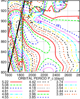
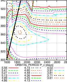
From now on, we consider three main models of the RV data for HD37124. All models incorporate three common Keplerian terms as in the eq. (3), the constant velocity terms (separate for the three datasets), and the annual term for the ELODIE dataset. The first RV model (I) does not incorporate anything else and thus has $d=20$ degrees of freedom. The second one (II) incorporates also an annual term for the Keck dataset and has $d=22$. The third one (III) incorporates the same terms as (I) plus a linear trend (common for all the three datasets) and thus has $d=21$. For all these models, the ratio $d/N\approx 0.16$ means that we are left with only $\approx 6$ observations per one parameter to be estimated. This indicates that the problem of obtaining a suitable orbital configuration of the system cannot be solved easily. Let us try to reconstruct the topological structure of the multidimensional graph of the likelihood function (6). Since the dimension of the problem is large, we cannot look on corresponding hypersurface directly. Let us pick two (of $d$) free parameters $x,y$ (say the orbital periods $P_{c}$ and $P_{d}$ of the outer planets). Then we consider the function $\tilde{l}^{\prime}(x,y)=\min\tilde{l}$, where the minimization of the goodness-of-fit function $\tilde{l}$ is performed over the rest of free parameters. This means that for any manually assigned values of $x,y$ we obtain corresponding best-fitting values of other parameters and find corresponding goodness-of-fit measure $\tilde{l}$. Further, the resulting function of two variables can be visualised on a two-dimensional grid.

Figure 2: Contour maps of the likelihood goodness-of-fit statistic $\min\tilde{l}$ for RV fits of HD37124. The maps are plotted in the plane of orbital periods $P_{c}$ and $P_{d}$ (measured in days). For each point in these panels, the likelihood goodness-of-fit function $\tilde{l}$ was minimized over the rest of free parameters. Thick straight line mark the position of the 2/1 MMR. The level values of the plotted function are shown below the respective panels. The panels in different columns correspond to the different RV models (model I, model II, model III, from left to right). The top raw of panels corresponds to the fits based on the whole accessible data array, whereas the bottom raw corresponds to the fits based on the Keck data only. Note the differences in period ranges shown in top and bottom graphs.

Table 1: Best-fitting orbital solutions for the planetary system around HD 37124.

parameter	IA, 2/1	IB	IIA, 2/1	IIB	IIIA, 2/1	IIIB
planet b
$P$ [days]	$154.37(13)$	$154.48(12)$	$154.53(12)$	$154.58(12)$	$154.37(13)$	$154.49(12)$
$\tilde{K}$ [m/s]	$28.39(82)$	$28.49(85)$	$27.42(73)$	$28.39(85)$	$28.06(83)$	$27.98(81)$
$\lambda$ [o]	$117.7(1.9)$	$119.1(1.8)$	$118.2(1.8)$	$118.8(1.7)$	$118.0(1.8)$	$120.2(1.7)$
$e$	$0.116(33)$	$0.116(33)$	$0.108(29)$	$0.081(27)$	$0.093(33)$	$0.064(28)$
$\omega$ [o]	$131(15)$	$132(23)$	$134(14)$	$132(23)$	$135(18)$	$140(25)$
$m\sin i$ [$M_{Jup}$]	$0.635(46)$	$0.637(47)$	$0.613(44)$	$0.635(46)$	$0.628(46)$	$0.626(46)$
$a$ [AU]	$0.518(17)$	$0.519(17)$	$0.519(17)$	$0.518(17)$	$0.518(17)$	$0.518(17)$
planet d
$P$ [days]	$912.5(7.7)$	$867.7(9.1)$	$902.3(8.7)$	$869.3(9.5)$	$904(14)$	$868.3(8.5)$
$\tilde{K}$ [m/s]	$13.8(1.2)$	$13.3(1.0)$	$15.1(1.0)$	$13.70(97)$	$13.1(1.1)$	$14.1(1.0)$
$\lambda$ [o]	$290.3(7.4)$	$345.9(4.3)$	$289.5(5.4)$	$344.7(4.2)$	$297.8(8.3)$	$346.0(4.0)$
$e$	$0.505(88)$	$0.056(72)$	$0.441(65)$	$0.207(87)$	$0.39(10)$	$0.025(68)$
$\omega$ [o]	$283(12)$	$75(77)$	$276(13)$	$49(19)$	$288(17)$	$390(150)$
$m\sin i$ [$M_{Jup}$]	$0.559(61)$	$0.528(54)$	$0.609(60)$	$0.545(53)$	$0.527(58)$	$0.560(55)$
$a$ [AU]	$1.695(57)$	$1.639(56)$	$1.682(57)$	$1.641(56)$	$1.684(59)$	$1.639(56)$
planet c
$P$ [days]	$1782(41)$	$1985(50)$	$1777(24)$	$1980(55)$	$1776(41)$	$1940(56)$
$\tilde{K}$ [m/s]	$14.9(1.1)$	$17.1(2.5)$	$15.2(1.0)$	$17.5(2.4)$	$14.2(1.2)$	$16.7(2.4)$
$\lambda$ [o]	$319.8(6.1)$	$309.3(5.2)$	$322.5(4.5)$	$312.7(4.6)$	$311.9(7.1)$	$306.2(5.7)$
$e$	$0.527(70)$	$0.593(85)$	$0.563(56)$	$0.555(72)$	$0.467(83)$	$0.573(84)$
$\omega$ [o]	$256.2(9.6)$	$325.8(7.6)$	$251.9(6.6)$	$335.0(8.2)$	$247(13)$	$320.9(8.7)$
$m\sin i$ [$M_{Jup}$]	$0.754(77)$	$0.895(61)$	$0.766(72)$	$0.915(62)$	$0.720(76)$	$0.867(59)$
$a$ [AU]	$2.648(97)$	$2.85(11)$	$2.643(91)$	$2.94(11)$	$2.642(97)$	$2.80(11)$
$c_{1}$ [$\frac{\rm m}{\rm s\cdot\rm yr}$]	-	-	-	-	$0.58(33)$	$0.78(27)$
ELODIE dataset
$c_{0}$ [m/s]	$65.5(4.3)$	$62.7(4.2)$	$66.5(4.5)$	$61.2(4.5)$	$67.4(4.4)$	$65.6(4.3)$
$A$ [m/s]	$17.6(3.2)$	$17.8(2.6)$	$17.5(3.5)$	$16.9(2.6)$	$18.2(3.5)$	$17.2(2.9)$
$\tau$ [days]	$167(20)$	$178(20)$	$164(20)$	$-181(22)$	$162(18)$	$171(20)$
$\sigma_{\star}$ [m/s]	$6.6(2.3)$	$5.9(2.3)$	$7.4(2.3)$	$6.5(2.3)$	$6.3(2.3)$	$5.6(2.4)$
r.m.s. [m/s]	$11.85$	$10.96$	$12.23$	$11.21$	$11.79$	$10.45$
CORALIE dataset
$c_{0}$ [m/s]	$4.3(4.2)$	$7.9(4.2)$	$4.8(4.3)$	$7.4(4.2)$	$5.3(4.4)$	$8.6(4.4)$
$\sigma_{\star}$ [m/s]	$11.3(4.0)$	$10.9(4.0)$	$12.3(4.2)$	$11.2(4.1)$	$12.1(4.1)$	$12.0(4.1)$
r.m.s. [m/s]	$17.45$	$16.93$	$17.62$	$16.73$	$17.68$	$17.38$
Keck dataset
$c_{0}$ [m/s]	$7.56(90)$	$9.11(84)$	$6.8(1.0)$	$10.8(1.1)$	$7.47(80)$	$9.00(79)$
$A$ [m/s]	-	-	$4.5(1.4)$	$3.8(1.6)$	-	-
$\tau$ [days]	-	-	$-148(19)$	$102(14)$	-	-
$\sigma_{\star}$ [m/s]	$2.58(54)$	$2.48(55)$	$1.24(71)$	$2.02(56)$	$2.44(54)$	$2.01(57)$
r.m.s. [m/s]	$3.704$	$3.713$	$3.044$	$3.381$	$3.566$	$3.359$
$d$	$20$		$22$		$21$
$\tilde{l}$ [m/s]	$8.269$	$8.025$	$7.816$	$7.888$	$8.180$	$7.711$
$\mathcal{C}$	$213$	$54$	$190$	$74$	$145$	$81$

The values of $c_{0}$ for ELODIE and CORALIE are given relatively to their first measuments. The uncertainties of the estimations are given in the brackets (e.g., $0.30(10)$ means $0.30\pm 0.10$, and $30.0(1.0)$ means $30.0\pm 1.0$). The values for the mean longitudes $\lambda$ and time shift parameters $\tau$ are given for the epoch $JD2452000$. The uncertainties of the minimum masses $m\sin i$ and of the semi-major axes $a$ incorporate the $10\%$ uncertainty of the stellar mass. The estimations of the effective RV jitters $\sigma_{\star}^{2}$ incorporate an analytic correction of the statistical bias as discussed in (Baluev, 2008c).

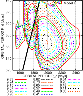
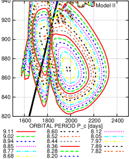
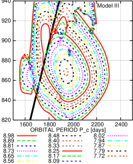
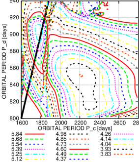
Fig. 2 shows such plot in the plane of orbital periods $P_{c}$ and $P_{d}$. We can see that the likelihood function constructed from the full available dataset (top panels of Fig. 2) has two main maxima with comparable values of $\tilde{l}$. The first one is centred on $P_{c}\approx 2000$ days and $P_{d}\approx 870$ days, and the second one on $P_{c}\approx 1800$ days and $P_{d}\approx 900$ days. We can see that the latter solution is close to the 2/1 MMR of the outer planets. Such orbital configurations are remarkable because only low-order MMRs can prevent planets on high-eccentricity orbits from close approaches and hence can make the whole system stable. This ‘double-headed’ shape of the likelihood function looks rather stable with respect to the choice of the RV model. From now on, we consider mainly the two mentioned families of solutions: the first one corresponds to the resonance 2/1 between planets ‘c’ and ‘d’, the second one is outside of this resonance (but may cover some other MMRs of relatively low, e.g. 7/3 and 5/2). Hereafter, we use the notation ‘A’ for the first family and ‘B’ for the second one. The full sets of estimated parameters for the three RV models are shown in Table 1. The respective minimum values of $\tilde{l}$ depend on the model adopted. For the models I and III, the ‘B’ solution provides formally better fit to the RV data in comparison with the ‘A’ one, but for the model II the corresponding values of $\tilde{l}$ are similar. Either model II or model III provide some improvement in the goodness-of-fit $\tilde{l}$, with respect to the model I. Let us note that the similar structure of the likelihood function can be also seen in the graphs constructed in the similar way for the RV model I, but with the use of the Keck data only (left-bottom panel in Fig. 2). However, the shape of the likelihood surface is more complicated in this case: the broad (much broader than in the top pictures) peak corresponding to the B-family is actually ‘double-headed’ itself (i.e., it consists of two close peaks having $P_{d}\approx 850$ days and $P_{d}\approx 820$ days). Moreover, the shape of the likelihood function constructed with the use of the Keck data only is severely dependent on the adopted RV model. For the model II, the B-family peak is clearly split into two distinct and very distorted peaks (one with $P_{c}\approx 1900$ days, $P_{d}\approx 870$, and another one with $P_{c}\approx 2200$ days and $P_{d}$ less than $800$ days, see middle-bottom panel in Fig. 2). For the model III, all the former peak are merged into a single very broad peak (formally centred not far from the the 2/1 MMR), which is continued to infinite $P_{c}$ (right-bottom panel in Fig. 2). Such behaviour, the further splitting of the local likelihood maxima and their severe sensitivity to the RV model, indicates that the analysis of the Keck data alone would yield significantly less reliable results than the joint analysis of all available data. However, even with the use of the full RV dataset, almost all of the best fits possess large values of the condition number $\mathcal{C}$, especially for the ‘A’ solution. This means that we should treat our results with a more care. In fact, no one of the best (in the sense of the goodness-of-fit measure) fits from Table 1 can be accepted. The values of the eccentricity $e_{c}$ (and often those of the $e_{d}$ as well) are large and lead to a very soon disintegration of the corresponding orbital configurations. For comparison, Table 2 contains the estimations of parameters for the system with the eccentricity $e_{c}$ or both the eccentricities $e_{c},e_{d}$ fixed at zero. These fits have much smaller values of $\mathcal{C}$, though worse goodness-of-fit. Numerical integration showed their dynamical stability and regular evolution on the time scales of (at least) $10^{6}$ yr, except for the fit II^′A which showed some signs of chaoticity at the time scale of $\sim 10^{5}$ yr, evidently due to a large $e_{d}=0.337$. It is important that only the ‘A’ group of solutions contains best-fitting circular orbits: the best-fitting solutions from the ‘B’ group approach the 2/1 MMR and softly turn into ‘A’ group of solutions when $e_{c}$ decreases.

Table 2: Low-eccentricity orbital solutions for the planetary system around HD 37124.

parameter	I′A, 2/1	I′′A, 2/1	II′A, 2/1	II′′A, 2/1	III′A, 2/1	III′′A, 2/1
planet b
$P$ [days]	$154.34(12)$	$154.31(12)$	$154.52(12)$	$154.36(13)$	$154.35(11)$	$154.34(11)$
$\tilde{K}$ [m/s]	$28.81(97)$	$28.27(96)$	$27.60(92)$	$29.32(97)$	$27.96(83)$	$28.20(82)$
$\lambda$ [o]	$117.4(2.0)$	$117.1(1.9)$	$117.0(1.8)$	$117.0(1.9)$	$118.6(1.7)$	$118.5(1.7)$
$e$	$0.078(32)$	$0.080(32)$	$0.090(28)$	$0.084(31)$	$0.062(29)$	$0.065(29)$
$\omega$ [o]	$132(23)$	$131(23)$	$116(19)$	$124(22)$	$146(25)$	$147(24)$
$m\sin i$ [$M_{Jup}$]	$0.644(48)$	$0.654(48)$	$0.617(46)$	$0.656(48)$	$0.625(46)$	$0.631(46)$
$a$ [AU]	$0.518(17)5$	$0.518(17)4$	$0.518(17)9$	$0.518(17)5$	$0.518(17)5$	$0.518(17)5$
planet d
$P$ [days]	$908(11).0$	$905(11).8$	$899.3(6.9)$	$904(12).1$	$883(10).7$	$881.9(8.5)$
$\tilde{K}$ [m/s]	$15.2(1.1)$	$14.17(92)$	$17.1(1.2)$	$14.13(94)$	$15.65(88)$	$15.21(81)$
$\lambda$ [o]	$322.3(4.1)$	$324.3(4.4)$	$322.9(3.2)$	$324.3(4.3)$	$328.9(3.6)$	$329.8(3.6)$
$e$	$0.174(88)$	$0($fixed$)$	$0.337(71)$	$0($fixed$)$	$0.095(71)$	$0($fixed$)$
$\omega$ [o]	$349(21)$	-	$1.7(9.8)$	-	$358(33)$	-
$m\sin i$ [$M_{Jup}$]	$0.614(62)$	$0.572(53)$	$0.689(66)$	$0.570(54)$	$0.626(54)$	$0.608(52)$
$a$ [AU]	$1.690(58)1$	$1.687(58)4$	$1.679(57)3$	$1.685(58)2$	$1.659(57)8$	$1.657(56)6$
planet c
$P$ [days]	$1810(41).3$	$1839(50).0$	$1759(28).0$	$1834(54).7$	$1815(40).0$	$1822(44).7$
$\tilde{K}$ [m/s]	$13.4(1.3)$	$12.0(1.1)$	$15.4(1.5)$	$11.9(1.0)$	$12.5(1.1)$	$11.86(88)$
$\lambda$ [o]	$310.7(4.7)$	$308.5(5.2)$	$318.8(3.7)$	$310.5(5.2)$	$303.0(5.1)$	$301.8(4.7)$
$m\sin i$ [$M_{Jup}$]	$0.682(81)$	$0.611(67)$	$0.774(89)$	$0.607(67)$	$0.638(68)$	$0.604(60)$
$a$ [AU]	$2.678(98)0$	$2.70(10)61$	$2.627(92)3$	$2.70(10)19$	$2.682(98)5$	$2.690(99)1$
$c_{1}$ [$\frac{\rm m}{\rm s\cdot yr}$]	-	-	-	-	$1.18(26)$	$1.22(24)$
ELODIE dataset
$c_{0}$ [m/s]	$64.2(4.3)$	$64.9(4.3)$	$63.9(4.5)$	$65.0(4.4)$	$68.4(4.5)$	$69.1(4.3)$
$A$ [m/s]	$18.9(3.1)$	$19.9(3.3)$	$17.8(3.3)$	$19.8(3.4)$	$18.9(3.7)$	$19.5(3.7)$
$\tau$ [days]	$167(18)$	$164(17)$	$167(20)$	$164(17)$	$158(17)$	$156(16)$
$\sigma_{\star}$ [m/s]	$6.8(2.2)$	$7.1(2.2)$	$7.6(2.2)$	$7.4(2.2)$	$6.7(2.3)$	$6.7(2.2)$
r.m.s. [m/s]	$11.95$	$12.33$	$12.53$	$12.45$	$12.08$	$12.18$
CORALIE dataset
$c_{0}$ [m/s]	$5.0(4.2)$	$4.5(4.0)$	$5.1(4.5)$	$4.2(4.0)$	$6.5(4.5)$	$6.3(4.3)$
$\sigma_{\star}$ [m/s]	$11.6(4.0)$	$10.5(3.8)$	$12.8(4.2)$	$10.3(3.9)$	$12.7(4.1)$	$12.1(4.0)$
r.m.s. [m/s]	$17.42$	$16.76$	$17.68$	$16.53$	$17.67$	$17.35$
Keck dataset
$c_{0}$ [m/s]	$7.56(75)$	$7.89(76)$	$9.52(93)$	$8.9(1.0)$	$7.88(61)$	$8.04(61)$
$A$ [m/s]	-	-	$4.9(1.3)$	$2.0(1.4)$	-	-
$\tau$ [days]	-	-	$134(13)$	$103(34)$	-	-
$\sigma_{\star}$ [m/s]	$3.36(55)$	$3.51(56)$	$2.21(55)$	$3.41(55)$	$2.15(56)$	$2.21(57)$
r.m.s. [m/s]	$4.218$	$4.319$	$3.436$	$4.193$	$3.394$	$4.446$
$d$	$18$	$16$	$20$	$18$	$19$	$17$
$\tilde{l}$ [m/s]	$8.710$	$8.776$	$8.280$	$8.769$	$8.065$	$8.057$
$\mathcal{C}$	$34$	$29$	$40$	$32$	$36$	$31$

The same notes as in Table 1 to be applied here. In these fits, the eccentricity $e_{c}$ or both the eccentricities $e_{c}$ and $e_{d}$ were fixed at zero. All these configurations correspond to the 2/1 MMR. The estimations of the semi-major axes and orbital periods are given with one or two excessive decimal digits (shown after two-digit uncertainties enclosed in brackets) to allow an unambigious reproducing of the long-term dynamics of these configurations (see Section 3.1). For example, $1810(41).3$ means $1810.3\pm 41$ and $2.70(10)19$ means $2.7019\pm 0.10$.

From the interplay of the indicators $\mathcal{C}$ and $\tilde{l}$ described above, we derive the following conclusion. Although the orbital fits from Table 1 show relatively small scatter of the residuals, this small scattering is in fact fictitious, as indicated by the corresponding values of $\mathcal{C}$. The number of RV data points and their temporal coverage still cannot constrain the full set in the model parameters reliably. The full RV model is ‘overloaded’. Injecting some kind of a priori information (e.g., fixing the eccentricities at low values) allows to overcome the obstacle of the statistical ill-determinacy. The resulting orbital fits possess better statistical reliability, but by the cost of some increase of the RV residuals scatter. Nevertheless, this increase is necessary to obtain a physically realistic orbital configuration. However, we cannot rule out the possibility that the actual orbits of the planets ‘c’,‘d’ are far from circular. To find more realistic orbital configurations than those from Table 1, but corresponding to eccentric orbits, we need to account for more subtle requirements of the dynamical stability in our analysis.

5 Dynamical interpretation

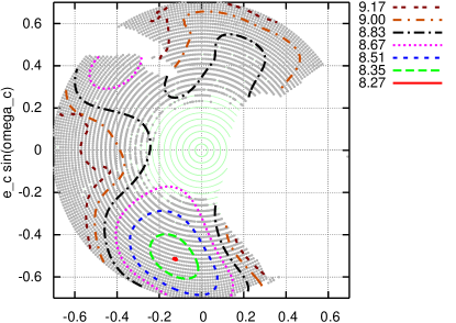
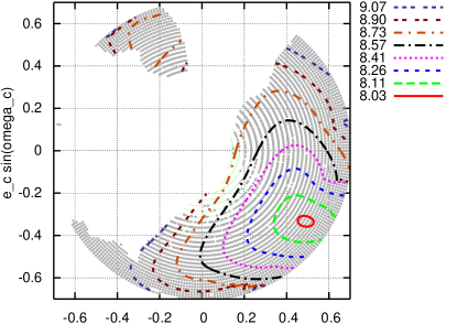
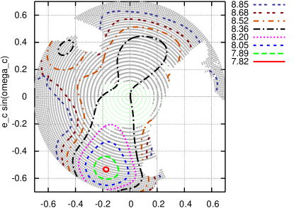
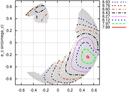
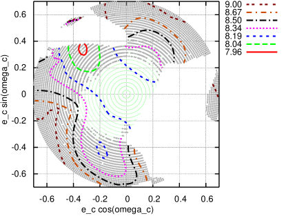
To obtain more realistic stable orbital configurations for this planetary system, we continue to use the method of planar plots of partially minimized goodness-of-fit statistic $\tilde{l}$. But now we examine orbital solution from a two-dimensional grid more carefully: for each solution, we perform a numerical integration in order to rule out rapidly disintegrating configurations. To perform such integrations, we need to know true masses of planets in the system. As it can be seen from (4), they depend on the mass of the star $M_{\star}$ and on the orbital inclinations. Following Vogt et al. (2005), we adopt $M_{\star}=0.78M_{\odot}$ with an uncertainty of $10\%$. Unfortunately, using the Keplerian RV model we can estimate only the minimum masses $m\sin i$ where the inclination $i$ remains unknown. Until the gravitational interactions between planets in the system are directly observed in the RV curve, the best thing that we can do is to assume a priori that the orbits are coplanar with $i=90^{\circ}$. If the actual inclination is less than $90^{\circ}$, the true masses of the interacting planets become larger and the stability region of the system become more narrow than for the edge-on configurations. The same effect is expected from non-zero mutual inclinations of the orbits, due to the well-known phenomenon of the $e$–$i$ coupling. Since much troubles in obtaining a realistic orbital configuration of the system are due to the large eccentricity of the outermost planet, let us firstly consider the plane of eccentric variables $(e_{c}\cos\omega_{c},e_{c}\sin\omega_{c})$. The corresponding maps are plotted in Fig. 3. We can see clearly the sophisticated shape of the likelihood surface: among the ‘A’ families of solutions, no one possess a single maximum. Instead, we can see 2-3 local maxima; all of them correspond to large values of $e_{c}$. The ‘B’ family shows single maximum, but again at large $e_{c}$. No one of these local maxima corresponds to a stable configuration. Stable solutions occupy only regions of small or moderate $e_{c}$. It is important to note that the small-eccentricity solutions correspond to the ‘A’ configuration only: when $e_{c}$ decreases, a B-type solution approach the 2/1 resonance and softly turns into an A-type one.

Figure 3: Contour maps of the likelihood goodness-of-fit statistic for RV fits of HD37124. These maps are plotted on the plane $(e_{c}\cos\omega_{c},e_{c}\sin\omega_{c})$ in the same way as in Fig. 2. Solutions which correspond to orbital configurations disintegrating in less than $30000$ years are marked by bold grey dots, other solutions are marked by fine (green in the electronic version of the paper) dots. These dots are arranged according to the polar coordinate system. Plots in the left column correspond to the ‘A’ solutions close to the 2/1 resonance (with no more than $5\%$ relative deviation of the period ratio), plots in the right column correspond to the ‘B’ solutions. The white regions (where $e_{c}<0.7$) mark the points for which the fitting algorithm could not find a solution from the corresponding family and switched to another one (that appeared significantly more likely). The ‘A’ and ‘B’ families of solutions overlap in the region of large $e_{c}$ without possibility of any smooth seam, but they seem to be sewed smoothly in the region of small $e_{c}$. The top, middle, and bottom pairs of panels correspond to the RV models I, II, and III, respectively.

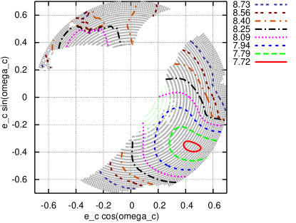As it can be seen from Fig. 3, we can easily find stable solutions from the ‘A’ family. Such solutions can possess values of $\tilde{l}$ as small as $\approx 8.6$ m/s (model I), $\approx 8.2$ m/s (model II), and $\approx 8.1$ m/s (model III). It is interesting that the region of stable configurations is somewhat correlated with one of the local minima of $\tilde{l}$ in the ‘A’ layer, located in the third quadrant of the coordinate plane. On contrary, we face much difficulties with obtaining a stable configuration from the family ‘B’. The main reason for almost all ‘B’ solutions to be unstable is that the best-fitting period ratio $P_{c}/P_{d}\approx 2.1-2.3$ is quite small and is not fixed (with a necessary precision) at any MMR of low order.

tabular@c@

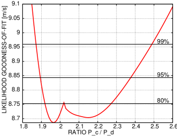
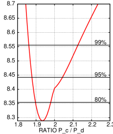
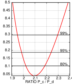
Contour maps of the likelihood goodness-of-fit statistic for RV fits of HD37124. These maps are plotted on the plane $(P_{c},e_{c})$ in the same way as in Figs. 2 and 3. Three panels correspond to the models I, II, and III (from top to bottom). In each of these panels, the A and B families of solutions were merged in a single plot. The bold nearly vertical lines mark the solutions having ratio of the best fitting periods $P_{c}$ and $P_{d}$ close to the 2/1, 7/3, 5/2, and 8/3 commensurabilities (lines from left to right). To locate stable solutions from the ‘B’ group, we use another pair of variables. In Fig. 5, the partially minimized $\tilde{l}$ is plotted in the plane $(P_{c},e_{c})$. We can see that the fits with low $e_{c}$ and with $P_{c}$ fixed far from the 2/1 resonance, possess uncomfortably large values of $\tilde{l}$. Fig 4 illustrates this more clearly. In this figure, we plot the function $\tilde{l}$, minimized so that the eccentricity $e_{c}$ was fixed at a safe value of $0.15$ and the period ratio $P_{c}/P_{d}$ was fixed at the values marked on the abscissas. Since the value of the eccentricity was fixed at a small value, the effects of the RV model non-linearity are significantly suppressed (it follows from relatively small values of $\mathcal{C}$ in Table 2), and thus we may try to find some confidence intervals for the ratio $P_{c}/P_{d}$ using the standard asymptotic ($N\to\infty$) theory of point estimations. We can see that the values $P_{c}/P_{d}>2.5$ and $P_{c}/P_{d}<1.87$ are beyond the $99\%$ confidence interval, when we use the RV model I. For the other RV models, this confidence interval becomes even smaller: $P_{c}/P_{d}\in[1.86,2.11]$ for the model II and $P_{c}/P_{d}\in[1.95,2.3]$ for the model III. When the eccentricity $e_{c}$ decreases, these confidence regions are shrinking around $P_{c}/P_{d}=2$.

Figure 4: Graphs of the likelihood goodness-of-fit function $\tilde{l}$, which was minimized so that the eccentricity $e_{c}$ was fixed at $0.15$ and the ratio of orbital periods $P_{c}/P_{d}$ was fixed at the values shown on the abscissas. Three panels correspond to the RV model I, II, and III (from left to right). The bold horizontal lines shows the levels of $\min\tilde{l}$ yielding the $80\%$, $95\%$, and $99\%$ asymptotic confidence intervals for $P_{c}/P_{d}$. These levels correspond to the values of the likelihood ratio statistic, which provide the asymptotic false alarm probabilities as small as $20\%$, $5\%$, and $1\%$ (see Baluev, 2008c).

However, we can note a promising region of high-eccentricity solutions near the resonance $5/2$ of the two outer planets. Surprisingly, numerical integration of the best fitting configuration with $P_{c}$ fixed at $2170$ days and $e_{c}$ fixed at $0.4$ (in the RV model I) showed a quite regular evolution without any signs of instability at the time scale of at least $10^{6}$ years. The evolution of this orbital configuration is a large-amplitude oscillation around an antialigned apsidal corotation, Therefore, this solution belongs to the class of orbital configurations in the 5/2 MMR found in (Goździewski et al., 2006) using only the Keck data. It seems that, due to the non-linearity of the RV models coupled with lack of the data and insufficient time coverage, none of the local minima of $\tilde{l}$ lies near the real orbital configuration of this system. Probably, these multiple local minima are only the fictitious ‘ripples’ produced by the lack of the observations. All these ‘ripples’ are located deeply in the zone of dynamical instability, and therefore cannot be close to the real configuration of the system. It is possible to find strictly the best-fitting orbital solution(s) simultaneously satisfying the stability requirement. Evidently, such solutions would be attracted by one of the ‘ripples’, and therefore would be close to the boundary of the domain of system stability. Therefore, we would have to deal with large difficulties concerning the very complicated structure of the parameter space near such boundaries (see, e.g., Goździewski et al., 2008), which probably represents the Arnold web (see, e.g, Froeschlé et al., 2006). Near such boundaries, the dynamics of the system is very sensitive to small changes of parameters, the stability map of the parametric space is strongly irregular, and hence the resolution of the parameter space should be chosen dense enough. This requires very time-consuming calculations for checking the stability of probe orbital configurations in this region. On contrary, it does not look likely that real planetary systems can be found in such extremely dynamically active regions: it would be rather difficult to explain how the system could migrate (without disintegration) to such a state through the dense web of the instability threads and why it stopped in a thin island of stability instead of moving further to dynamically unstable configurations. Therefore, the reliability of such ‘hardly-stable’ solutions would be too low to justify the associated time-consuming calculations. In addition, considering the boundary of the stability domain, it is rather difficult to understand the physical mechanism stabilizing the configurations in the given domain. In this paper, following Hadjidemetriou (2006), we will pay more attention to the centres of the stability domains which point out families of orbital configurations having some ‘stock of stability’. For having a clear picture of possible dynamical regimes of a planetary system, it is the position of the centre of the stability domain which should be located and for which we should know possible uncertainties. Considering the kernel of a stability domain, we avoid dealing with the sophisticated dynamical structure near its boundary, which is hardly able to carry much information about the dynamics of the real system. When an orbital solution has some stock of stability, the dynamics of the corresponding planetary configuration is much more regular and much less sensitive to small changes of parameters. To obtain such orbital solutions, we will try to decrease the dimension of the problem (i.e., the number of degrees of freedom $d$) using certain a priori information about the stability of resonance planetary systems.

6 The value of apsidal corotation resonances

Bearing in mind the results by Ji et al. (2003); Hadjidemetriou (2006, 2008); Voyatzis & Hadjidemetriou (2006), let us recall that regular stable motions on high-eccentricity orbits with small period ratio are only possible if the planets are trapped in a MMR and simultaneously are close to (or, at least, not far from) an apsidal corotaion resonance. The details of the theory of apsidal corotation resonances, along with necessary formulae and further references can be found, for instance, in (Beaugé et al., 2003). For a brief summary, let us consider two planets trapped in the $p/q$ MMR, i.e. having the ratio of orbital periods $P_{2}/P_{1}\approx p/q$ with $p>q$. We can write down the resonant angles

$$s_{1}=\frac{p\lambda_{2}-q\lambda_{1}}{p-q}-\omega_{1},\qquad s_{2}=\frac{p\lambda_{2}-q\lambda_{1}}{p-q}-\omega_{2}$$ (10)

and the canonically conjugated action variables

$$I_{1}=L_{1}\left(1-\sqrt{1-e_{1}^{2}}\right),\qquad I_{2}=L_{2}\left(1-\sqrt{1-e_{2}^{2}}\right),$$ (11)

where $\lambda_{i}$ are the mean longitudes of the planets and $L_{i}\simeq m_{i}\sqrt{a}_{i}$ are the Delaunay action variables. After averaging the Hamiltonian $H$ of the system over the fast variables (i.e, over the mean longitudes $\lambda_{i}$) keeping the resting slow ones, the resulting averaged Hamiltonian $\langle H\rangle$ depends on the canonical variables $s_{i},I_{i}$, and (as on parameters) on the masses $m_{i}$ of the planets. Evidently, this averaging accounts properly for the orbital resonance. The averaged equations of motion are then given by

$$\frac{dI_{i}}{dt}=-\frac{\partial\langle H\rangle}{\partial s_{i}},\qquad\frac{ds_{i}}{dt}=\frac{\partial\langle H\rangle}{\partial I_{i}}$$ (12)

Suppose that some values $s_{i}^{*},I_{i}^{*}$ determine the position of an extremum of $\langle H\rangle$. We can easily see that every such extremum provides a stationary solution $s_{i}\equiv s_{i}^{*},I_{i}\equiv I_{i}^{*}$ of the averaged system (12). Such stationary solution is often called ‘apsidal corotation resonance’ (hereafter ACR). If the initial state of the planetary system slightly deviates from an exact ACR, the motion is a stable oscillation around the exact stationary solution, because the planets are prevented from close approaches. If the orbits of planets are highly eccentric and are far from stationary solutions of the averaged Hamiltonian equations, the motion is, most probably, highly chaotic and unstable: the secular drift of resonant angles (10) leads the planets to too close approaches destabilizing the system. Stable solutions with one or both the resonant angles circulating are also possible in some cases; however, for high-eccentricity configurations, the ACRs mark centres of dynamical stability (see e.g. Hadjidemetriou, 2006, 2008). To obtain nominal orbital configurations of the system, we require from the resonant planets ‘c’ and ‘d’ to be locked in an exact ACR (while neglecting the influence of the innermost planet ‘b’). This can be justified not only by the stability considerations. Beaugé et al. (2006) showed that adiabatic dissipative perturbations (e.g., interaction with a protoplanetary disk) can cause planet pairs in a MMR to be captured in an ACR as well. The requirement of the ACR lock implies four algebraic equations: $\partial\langle H\rangle/\partial s_{c,d}=0$ and $\partial\langle H\rangle/\partial I_{c,d}=0$. We neglect here the gravitational influence of the innermost planet ‘b’: it is seemingly non-resonant with the outer planets and probably should not affect their resonant dynamics much. The four equations mentioned above put certain constraints on the full set of free parameters to be estimated from RV data and decrease the number of degrees of freedom by four. It is very important, because this decreasing makes the problem significantly better determined: we have about $8$ observations per a degree of freedom instead of about $6$.

Table 3: ACR fits for the planetary system around HD 37124.

parameter	IcA, 2/1	IcB, 5/2	IIcA, 2/1	IIcB, 5/2	IIIcA, 2/1	IIIcB, 5/2
planet b
$P$ [days]	$154.38(12)$	$154.36(12)$	$154.46(12)$	$154.36(13)$	$154.38(12)$	$154.35(12)$
$\tilde{K}$ [m/s]	$29.21(92)$	$28.9(1.0)$	$28.84(83)$	$28.9(1.0)$	$28.69(85)$	$28.8(1.0)$
$\lambda$ [o]	$119.3(1.9)$	$119.1(1.8)$	$118.8(1.7)$	$119.1(1.9)$	$120.1(1.8)$	$119.8(1.8)$
$e$	$0.079(32)$	$0.074(34)$	$0.095(29)$	$0.074(34)$	$0.066(31)$	$0.067(34)$
$\omega$ [o]	$130(23)$	$154(23)$	$119(18)$	$154(24)$	$136(26)$	$164(26)$
$m\sin i$ [$M_{Jup}$]	$0.653(48)$	$0.647(48)$	$0.645(47)$	$0.647(49)$	$0.642(47)$	$0.644(48)$
$a$ [AU]	$0.518(17)6$	$0.518(17)5$	$0.518(17)8$	$0.518(17)5$	$0.518(17)6$	$0.518(17)5$
planet d
$P$ [days]	$907.6(8.9)$	$874.6(7.8)$	$897.2(7.8)$	$874.4(8.2)$	$896(11).3$	$874.6(7.5)$
$\tilde{K}$ [m/s]	$16.10(81)$	$13.82(86)$	$16.53(81)$	$13.84(91)$	$16.63(78)$	$14.40(91)$
$\lambda$ [o]	$315.9(3.0)$	$340.7(3.6)$	$316.4(2.5)$	$340.7(3.7)$	$317.4(2.9)$	$339.7(3.5)$
$e$	$0.306(88)$	$0.221(26)$	$0.311(77)$	$0.221(26)$	$0.289(73)$	$0.199(33)$
$\omega$ [o]	$320.8(8.8)$	$154.5(8.4)$	$334.4(7.9)$	$154.6(8.5)$	$315(11)$	$154.0(8.6)$
$m\sin i$ [$M_{Jup}$]	$0.650(54)$	$0.551(50)$	$0.665(55)$	$0.552(51)$	$0.668(55)$	$0.574(53)$
$a$ [AU]	$1.689(57)7$	$1.648(56)3$	$1.676(57)8$	$1.648(56)1$	$1.675(58)6$	$1.648(56)4$
planet c
$P$ [days]	$1815(17).3$	$2186(20).4$	$1794(15).5$	$2186(21).0$	$1792(22).8$	$2187(19).0$
$\tilde{K}$ [m/s]	$12.6(1.1)$	$10.54(93)$	$12.8(1.1)$	$10.54(95)$	$12.5(1.0)$	$10.30(87)$
$\lambda$ [o]	$311.8(5.3)$	$301.0(5.5)$	$318.2(5.0)$	$301.0(5.6)$	$307.7(6.0)$	$300.3(5.5)$
$e$	$0.122(56)$	$0.377(74)$	$0.132(42)$	$0.379(78)$	$0.136(54)$	$0.333(76)$
$\omega$ [o]	$267(23)$	$334.5(8.4)$	$278(21)$	$334.6(8.5)$	$250(20)$	$334.0(8.6)$
$m\sin i$ [$M_{Jup}$]	$0.639(70)$	$0.570(63)$	$0.648(71)$	$0.570(64)$	$0.631(68)$	$0.558(60)$
$a$ [AU]	$2.683(91)0$	$3.03(10)69$	$2.662(90)4$	$3.03(10)66$	$2.660(91)8$	$3.03(10)75$
$c_{1}$ [$\frac{\rm m}{\rm s\cdot\rm yr}$]	-	-	-	-	$0.87(32)$	$0.44(26)$
ELODIE dataset
$c_{0}$ [m/s]	$64.7(4.4)$	$65.5(4.7)$	$64.6(4.6)$	$65.5(4.5)$	$67.4(4.5)$	$66.8(4.5)$
$A$ [m/s]	$18.8(3.1)$	$20.2(3.2)$	$18.1(3.3)$	$20.2(3.3)$	$18.4(3.4)$	$19.8(3.3)$
$\tau$ [days]	$169(19)$	$167(17)$	$168(20)$	$167(18)$	$163(18)$	$165(18)$
$\sigma_{\star}$ [m/s]	$7.2(2.2)$	$7.7(2.1)$	$8.2(2.1)$	$7.7(2.1)$	$6.8(2.2)$	$7.6(2.1)$
r.m.s. [m/s]	$12.20$	$12.60$	$12.85$	$12.51$	$12.15$	$12.33$
CORALIE dataset
$c_{0}$ [m/s]	$4.8(4.1)$	$6.2(3.8)$	$4.5(4.1)$	$6.1(3.8)$	$5.7(4.4)$	$6.3(3.9)$
$\sigma_{\star}$ [m/s]	$11.5(3.9)$	$9.4(3.8)$	$11.3(4.0)$	$9.4(3.8)$	$12.6(4.1)$	$10.0(3.8)$
r.m.s. [m/s]	$17.91$	$15.91$	$17.43$	$15.82$	$18.44$	$16.06$
Keck dataset
$c_{0}$ [m/s]	$7.13(73)$	$8.13(72)$	$9.1(1.0)$	$8.1(1.0)$	$7.11(66)$	$8.15(71)$
$A$ [m/s]	-	-	$3.9(1.3)$	$0.1(1.1)$	-	-
$\tau$ [days]	-	-	$131(17)$	-	-	-
$\sigma_{\star}$ [m/s]	$3.48(56)$	$3.15(56)$	$2.77(54)$	$3.27(55)$	$2.93(55)$	$3.08(55)$
r.m.s. [m/s]	$4.322$	$4.108$	$3.762$	$4.148$	$3.910$	$4.001$
$d$	$16$		$18$		$17$
$\tilde{l}$ [m/s]	$8.851$	$8.616$	$8.601$	$8.693$	$8.530$	$8.549$
$\mathcal{C}$	$39$	$56$	$38$	$64$	$48$	$79$

The same notes as in Table 1 to be applied here. These orbital elements were obtained for the Jacobi coordinate system with appropriate masses assigned to the reference barycentres. See Appendix A for more details concerning the algorithm used to obtain these fits. The semi-major axes and some orbital periods are given with excessive decimal digits, as in Table 2.

More detailed description of the algorithm used to obtain such ACR fits, is given in Appendix A. The resulting fits of ACR solutions are given in Table 3. It is important that since the position of the ACR depends on the planetary mass ratio only and is almost independent of the individual planet masses, the solutions from Table 3 are almost independent of the assumptions about the orbital inclination of the system: $(m_{c}\sin i)/(m_{d}\sin i)=m_{c}/m_{d}$. We only need to adjust the ratio of orbital periods by the quantity $\mathcal{O}(m/M_{\star})$ (see formula (22) in Appendix A), but this adjustment have insignificant effect on the RV fit quality (until we consider inclinations as small as a few degrees). This invariance with respect to orbital inclination represents an extra advantage of the use of the ACR fitting procedure.

Figure 5: Top panels: orbits of the HD37124 system for the ACR fits (model I only). Left panel is for the 2/1 MMR; right panel is for the 5/2 MMR. Straight solid lines mark the conjunction positions. Broken lines mark the lines of apses. Middle panels: contour maps of the averaged Hamiltonian $\langle H_{cd}\rangle$ in the planes of resonant angles $s_{d},s_{c}$, for the same MMRs and eccentricities as in top panels. Crosses mark the actual ACR positions corresponding to local maxima of $\langle H_{cd}\rangle$.

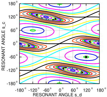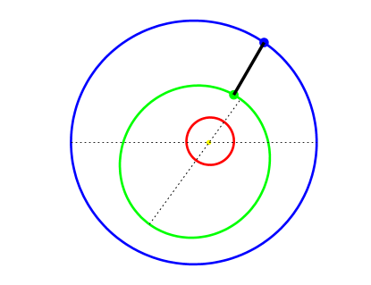
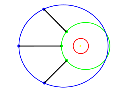
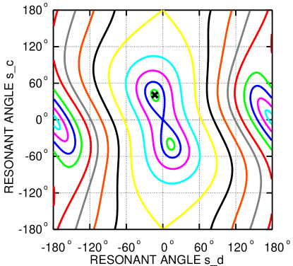
We can see that in the case of the 2/1 resonance, the best fitting ACR is asymmetric with difference between the longitudes of periastra about $60^{\circ}$, whereas in the case of the 5/2 resonance, the corresponding ACR is symmetric and antialigned (i.e., $\omega_{c}-\omega_{d}=180^{\circ}$), see Fig. 5. The corresponding RV curves fit all available RV data satisfactorily, including the ELODIE measurements (Fig. 6). The values of the goodness-of-fit measure $\tilde{l}$ are not increased very much with respect to those from Table 1 and are comparable with those from Table 2. This means that one of the ACR fits can reflect the true configuration of this system quite well. The corresponding condition numbers $\mathcal{C}$ for the 2/1 resonance in Table 3 are much less than in Table 1. This indicates that the topology of the likelihood surface becomes simpler and closer to the desirable paraboloidal one. The troubles connected with multiple local maxima of the likelihood have been overcome in the ACR fits. We can now say more definitely, that the effect of the putative annual term in the Keck RV data on the fit quality is similar to the effect of the linear RV trend (which could be due to a long-period planet or brown dwarf in the system). These extra terms are significant in the fits for the 2/1 resonance (the ‘A’ group of solutions). For these fits, the estimations of false alarm probabilities, calculated from the corresponding likelihood ratios according to Baluev (2008c), are about $2\%$ and $0.3\%$ (for the annual term and for the linear drift, respectively). The 5/2 resonance (B) solution does not require these terms in the RV model. This dilemma can be solved by future observations only.

tabular@c@

RV curves for the ACR solutions I^cA (top panel) and I^cB (bottom panel), plotted together with the RV measurements and their residuals. The error bars do not incorporate estimated values of the RV jitter. The best-fitting annual sinusoidal drift of the ELODIE measurements was preliminarily subtracted.

7 Long-term dynamics

Now we consider the dynamical regimes of our nominal orbital configurations more closely. We are especially interested in how much the innermost planet can disturb the apsidal corotation of the two outer planets. This effect may be split in two categories:

1. The planet ‘b’ can inspire some extra oscillation of the outer planets ‘c’, ‘d’ near their unperturbed ACR (‘unperturbed’ means obtained without taking into account the influence of the planet ‘b’).

2. The planet ‘b’ can shift the position of the libration centre from the unperturbed ACR.

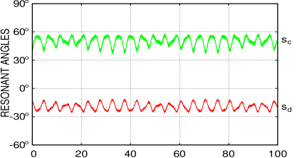
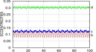
Only the first effect may significantly affect the system stability, because only a large-amplitude oscillation around the libration centre can significantly increase the probability of close approaches of the resonant planets.

Figure 6: Temporal evolution of the ACR configurations of planets in HD37124 (for RV model I only). Left panels show the evolution of the eccentricities, right panels show the evolution of resonant angles. Top pair: resonance 2/1, orbital parameters were taken from Table 3, solution I^cA. Middle pair: the same case, but the value of the mass $m_{c}$ was increased so that the value of $\tilde{K}_{c}$ increased by $1$ m/s. Bottom pair: resonance 5/2 (Table 3, solution I^cB). The same character of motion is conserved on the time scale of $10^{6}$ yr (and probably much longer) for all the cases.

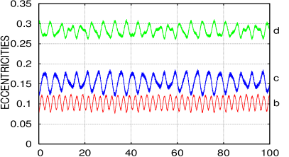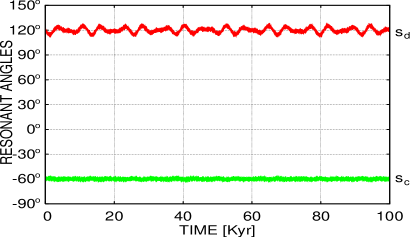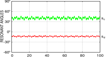
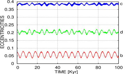
Fig. 6 illustrates both effects. We can see that the orbital configuration I^cA taken from Table 3 shows moderate oscillation of the eccentricities $e_{c},e_{d}$ and libration of resonant angles $s_{c},s_{d}$ around some equilibrium values. However, the centres of oscillations are somewhat shifted with respect to the unperturbed ACR. Heuristically, to counterbalance the gravitational influence of the perturbing planet ‘b’, we need to increase somewhat the mass of the outermost planet ‘c’. This assumption is confirmed by numerical integration: orbital configuration with $m_{c}$ increased by about $8\%$ shows much less libration amplidute. Moreover, this adjustment decreases the statistic $\tilde{l}$ by about $0.1$ m/s (i.e., the scatter of the data around the RV model becomes slightly less). In the case of the 5/2 resonance, (solution I^cB), the libration amplitude is quite small for the unperturbed ACR solution already. The evolution of these orbital configurations appears perfectly regular and does not show any instability at the time scale of at least $10^{6}$ yr. More detailed analysis shows a great diversity of dynamical behaviour in the vicinity of the ACR solutions. The amplitude and character of the librations can be different. For certain orbital configurations inside the 2/1 MMR, the system may switch (from time to time) between alternating asymmetric ACRs with $\omega_{c}-\omega_{d}\approx-60^{\circ}$ and $\omega_{c}-\omega_{d}\approx+60^{\circ}$. Librations surrounding simultaneously the pair of stable asymmetric stationary solutions and unstable symmetric aligned ACR (see the left-middle panel in Fig. 5) are also possible.

8 Testing the existence of extra planets

When the best fitting orbital structure of the planetary system appears unstable, we can suspect that more planets orbit the star. It was the case for the system of $\mu$ Ara: the determination of realistic orbits of $\mu$ Ara b and c represented an essential difficulty (e.g., Goździewski et al., 2005) until the discovery of the planet $\mu$ Ara e placed all in the places (Pepe et al., 2007; Goździewski et al., 2007). To test the hypothesis of an extra planet orbiting HD37124, we use the likelihood ratio–based periodogram described in the paper (Baluev, 2008c). This periodogram represent a generalization of the usual Lomb (1976)-Scargle (1982) periodogram (as well as of the data-compensated discrete Fourier transform periodogram by Ferraz-Mello (1981)) and incorporates a built-in estimation of the RV jitter.

Figure 7: The likelihood ratio periodograms of the RV residuals for different three-planet orbital models of the system of HD37124. Every value of these periodograms represents the modified likelihood ratio statistic (see Baluev, 2008c), calculated for the base model of the residuals (free constant velocity offsets + free common linear drift) and for the alternative model incorporating also a sinusoidal variation with free amplitude and phase. The panels in the left column represent the periodograms constructed from the residuals of full RV dataset. They were constructed in the range of periods starting from $10$ days, since the errors in the dates of ELODIE measurements do not allow to fit accurately more short periods. The graph in the right columns show the periodograms constructed for the Keck residuals only. The top pair of panels is for the ACR solution in the 2/1 MMR (RV model I). The bottom pair of panels is for the ACR solution in the 5/2 MMR (also RV model I). For the case of graphs to the left, the normalized frequency bandwidth $W\approx 350$, and for the graphs to the right $W\approx 3400$.

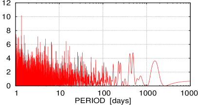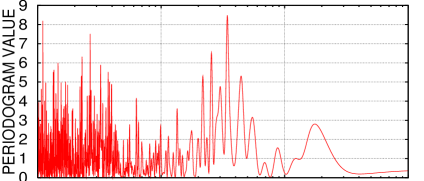
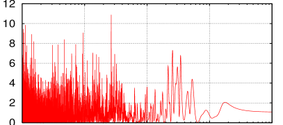
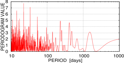
The graphs of such periodograms of RV residuals for several orbital solutions and involving different datasets are shown in Fig. 7. We can see that none of the peaks rises clearly beyond the apparent noise level. The formal significances of a periodogram peak can be assessed using the analytic expression for the associated false alarm probabilities (i.e., the probability to claim that the peak is statistically significant when actually it is a result of noise fluctuations) from the paper (Baluev, 2008a):

$$(\mathrm{false\ alarm\ probability})\approx We^{-z}\sqrt{z},$$ (13)

where $z$ is the height the maximum periodogram peak, and $W=f_{\rm max}T_{\rm eff}$ is the normalized frequency bandwidth, with $f_{\rm max}$ being the maximum frequency being scanned and $T_{\rm eff}$ being the effective time series span (which is usually close to the actual time base). The applicability of this formula to the likelihood ratio periodograms was also discussed in (Baluev, 2008c). None of the peaks on the periodograms in Fig. 7 possesses the false alarm probability estimation less than $\sim 20\%$. This means that no extra detectable periodicity is present in the RV data being used in our work. The only suspiciuous peak is shown by the periodogram of the residuals to the solution I^cA (the upper-right panel in Fig. 7). This peak is close to the period of $26.6$ days and possesses the false alarm probability of $\sim 2\%$, if the latter is calculated for the period range $P\geq 10$ days (instead of $P\geq 1$ days). However, this peak is not present in other periodograms and thus seems to be a noise artefact exacerbated by inaccuracies of the model of the RV curve for this orbital solution and by aliasing (caused by uneven spacings of the RV data), rather than to reflect an RV oscillation induced by an extra hypothetical planet. There is also possibility that the putative additional planets are also trapped in a MMR with one of the two outer planets. For example, the RV oscillation of the hypothetical fourth planet having orbital period of $P_{d}/2\approx 450$ days or $P_{c}/3\approx 650$ days would be extremely difficult to extract from the synthetic RV curve. Such RV oscillation could be almost equally treated as a Fourier overtone associated with Keplerian oscillations induced by the outer planets (thus resulting in some change of their best-fitting eccentricities). Since the currently available RV data for HD37124 do not allow reliable determination of the orbits in the system even for the three-planet configuration, the more complicated (and worse determined) four-planet configurations were not considered here. It is worth emphasizing that there is no necessity to call for four-planet configurations of HD37124. All present difficulties connected with this system can be explained from the positions of data analysis, that is by the lack of the RV data, which is not sufficient to constrain reliably the non-linear triple-planet RV model having large number of degrees of freedom. For example, it was shown by Baluev (2008b) that the unrealistically large formal estimations of the eccentricities can be interpreted as a result of their statistical (systematic) biasing.

9 Conclusions

In the paper, the full set of high-precision RV data available for the planetary system of HD37124 is analysed. The analysis involves different RV models and accounts for the requirement of the dynamical stability of the planetary system. The most likely orbital configurations of the system, found in the paper, are split in four classes:

1. Two outer planets ‘c’,‘d’ are captured in the 2/1 mean-motion resonance and move on orbits with low or moderate eccentricities ($e\lesssim 0.15$). The planets are far from an apsidal corotation resonance, but the whole system is still stable due to relatively low eccentricities.

2. The planets ‘c’,‘d’ are in the 2/1 mean-motion resonance and move on significantly elliptic orbits with moderate or high eccentricities. The system is stable, because the planets are locked in (or librate around) an asymmetric apsidal corotation.

3. The planets ‘c’,‘d’ are in the 5/2 mean-motion resonance. They move on elliptic orbits with high or moderate eccentricities. The planetary orbits are intersecting (or close to an intersection), but the system is stable, because the planets are locked in (or librate around) a symmetric antialigned apsidal corotation. This branch of solutions was also groped by Goździewski et al. (2006) basing on the Keck data only.

4. The planets ‘c’,‘d’ are not necessarily trapped in a mean-motion resonance. They move on orbits with relatively low eccentricities, which make the whole system stable. However, these solutions show larger scatter of the RV residuals and thus are less likely then solutions from other branches. When the eccentricies are fixed at small values, the ratio of the best fitting orbital periods of the two outer planets appears within a few per cent of the 2/1 MMR. The values of the period ratio $P_{c}/P_{d}$ exceeding $2.3-2.5$ are unlikely. However, the configurations with $P_{c}/P_{d}<2.3$ are quite possible, bearing in mind the example of the planets b and e in the system of $\mu$ Ara, which are close to, but likely not trapped in, the 2/1 MMR with $P_{b}/P_{e}\approx 2.1$ (Goździewski et al., 2007; Short et al., 2008).

The branches (2) and (3) are of a special interest, because we do not know examples of planetary systems with similar orbital configurations. The possibility of such orbital configurations makes the algorithms of optimal scheduling of RV observations (Baluev, 2008d; Ford, 2008) extremely tempting to use for this star. It was also shown that the RV residuals do not contain any detectable extra periodicity which could provide clear evidence for a fourth planet in the system. However, for the solutions close to the 2/1 MMR, there are evidences for an extra variation in the RV residuals. This variation can be explained by putative annual errors in the Keck data or, alternatively, by extra linear RV drift which could be induced by a distant unseen companion of the star.

Appendix A Obtaining ACR fits

Here we describe the procedure of obtaining the ACR fits in more details. The algorithm that we are about to describe may be useful also for other planetary systems. But before we proceed, we have to choose some coordinate system. Actually, in the case of HD37124, it may be checked that the offsets of resulting orbital parameters, referenced in different coordinate systems, would be quite negligible in the sense of the RV fit quality. However, the type of the coordinate system should be stated for the purposes of long-term integrations of the planetary system: the coordinate system used in the integration should match the given orbital elements. The actual choice of the Jacobi coordinates was motivated here by the fact noted in (Lissauer & Rivera, 2001; Lee & Peale, 2003), that it is Jacobi coordinate system in which the osculating orbital elements are mostly close to those obtained using the kinematic (Keplerian) RV model, especially when the system contains hierarchical planet pairs (like pairs of planets b–c and b–d in the case of HD37124). This property of the Jacobi coordinates may be useful, for instance, during a transition from multi-Keplerian to N-body model of the RV, that was (and probably will be) needed for some resonant planetary systems after accumulating a sufficiently long observation time span. In the Jacobi coordinates, the Hamiltonian of a system with $N$ planets looks like

$$H=\sum_{i=1}^{N}\left(\frac{{\vec{p}^{\prime}_{i}}^{2}}{2m^{\prime}_{i}}-\frac{Gm_{0}m_{i}}{r_{i}}\right)-\sum_{1\leq i<j\leq N}\frac{Gm_{i}m_{j}}{r_{ij}},$$ (14)

where $G$ is the gravitational constant, $m_{i}$ are the planetary masses, $r_{i}$ are the astrocentric distances of the planets, $r_{ij}$ are the distances between the planets, $\vec{p}^{\prime}_{i}$ are the Jacobi momenta and $m^{\prime}_{i}=m_{i}(\sum_{j=0}^{i-1}m_{j})/(\sum_{j=0}^{i}m_{j})$ are the Jacobi masses. Now we need to split (14) in the Keplerian part that we consider as unperturbed one and in the part that we consider as perturbational function. This may be done non-uniquely. We adopt the splitting $H=\sum_{i=1}^{N}H_{\mathrm{Kep},i}-\sum_{i=1}^{N}R_{i}$, where

$$H_{\mathrm{Kep},i}=\left(\frac{{\vec{p}^{\prime}_{i}}^{2}}{2m^{\prime}_{i}}-\frac{GM_{i-1}}{r^{\prime}_{i}}m_{i}\right),\qquad R_{i}=Gm_{i}\left(\sum_{j=i+1}^{N}\frac{m_{j}}{r_{ij}}+\frac{m_{0}}{r_{i}}-\frac{M_{i-1}}{r^{\prime}_{i}}\right).$$ (15)

Here $r^{\prime}_{i}$ is the length of the Jacobi radius-vector for the $i^{\rm th}$ planet, $M_{i-1}=\sum_{j=0}^{i-1}m_{j}$ is the sum of the star mass and of the masses of all planets being interior with respect to the given planet. Therefore, $H_{\mathrm{Kep},i}$ is chosen so that the corresponding unperturbed Keplerian orbit is referenced to a fictitious central body having mass $M_{i-1}$. We will use only the second-order approximation of the Hamiltonian. In this approximation, we represent $R_{i}=\sum_{j=i+1}^{N}R_{ij}+\mathcal{O}(m^{3})$, where

$$R_{ij}=Gm_{i}m_{j}\left(\frac{1}{|\vec{r}^{\prime}_{i}-\vec{r}^{\prime}_{j}|}-\frac{\vec{r}^{\prime}_{i}\cdot\vec{r}^{\prime}_{j}}{{r^{\prime}_{j}}^{3}}-\frac{1}{r^{\prime}_{j}}\right).$$ (16)

Here $\vec{r}^{\prime}_{i}$ are the Jacobi position vectors. This approximation for the case of two planets may be found in (Gerassimov et al., 1996, § 4.2), and the extension to $N\geq 3$ planets is straightforward. Let us define the following function of six input parameters:

$$\mathcal{R}(\alpha,e_{\rm inn},e_{\rm out},\lambda_{\rm inn},\lambda_{\rm out},\Delta\omega)=\frac{1}{|\vec{r}_{\rm inn}-\vec{r}_{\rm out}|}-\frac{\vec{r}_{\rm inn}\cdot\vec{r}_{\rm out}}{r_{\rm out}^{3}}-\frac{1}{r_{\rm out}}.$$ (17)

Here, the vectors $\vec{r}_{\rm inn}$ and $\vec{r}_{\rm out}$ describe positions of abstract ‘inner’ and ‘outer’ planets moving on Keplerian orbits. The Keplerian orbital elements marked by the subscript ‘$\rm inn$’ refer to the orbital elements of the inner planet, and quantitties marked by the subscript ‘$\rm out$’ correspond to the outer planet. The semi-major axis of the inner abstract planet is set to unit, and the semi-major axis of the abstract outer planet is equal to $\alpha$. The parameter $\Delta\omega=\omega_{\rm out}-\omega_{\rm inn}$ represents the difference between the longitudes of periastra. Then the obvious identity $R_{ij}=\frac{Gm_{i}m_{j}}{a_{i}}\mathcal{R}(a_{j}/a_{i},e_{i},e_{j},\lambda_{i},\lambda_{j},\omega_{j}-\omega_{i})$ holds true. As usually, the Keplerian parts of the Hamiltonian depend only on the Delaunay actions $L_{i}$ (and, as on parameters, on the masses of the planets) and remain unchanged by any averaging. Let us now restrict our attention to the motion of the (possibly) resonant planets HD37124 c and d, neglecting the influence of the innermost planet b. The perturbational function describing the interaction of the planets c and d is given by $\frac{Gm_{c}m_{d}}{a_{d}}\mathcal{R}(\alpha=a_{c}/a_{d},e_{d},e_{c},\lambda_{d},\lambda_{c},\Delta\omega=\omega_{c}-\omega_{d})$. The corresponding averaged perturbational function is then given by $\frac{Gm_{c}m_{d}}{a_{d}}\langle\mathcal{R}\rangle(\alpha,e_{d},e_{c},s_{d},s_{c})$, where the averaged function $\langle\mathcal{R}\rangle$ depends on only five input parameters $\alpha,e_{\rm inn},e_{\rm out},s_{\rm inn},s_{\rm out}$:

$$\langle\mathcal{R}\rangle(\alpha,e_{\rm inn},e_{\rm out},s_{\rm inn},s_{\rm out})=\int_{0}^{2\pi}\mathcal{R}\left(\alpha,e_{\rm inn},e_{\rm out},s_{\rm inn}+p\theta,s_{\rm out}+q\theta,s_{\rm inn}-s_{\rm out}\right)\frac{d\theta}{2\pi}.$$ (18)

Note that the last term in the expression (17) is averaged to $1/\alpha$. This term reflects only the fact that the osculating Keplerian orbits are refered to different fictitious central masses. In fact, we need to average only the resting classical expression of the perturbational function:

$$\langle\mathcal{R}\rangle=\left\langle\frac{1}{|\vec{r}_{\rm inn}-\vec{r}_{\rm out}|}-\frac{\vec{r}_{\rm inn}\cdot\vec{r}_{\rm out}}{r_{\rm out}^{3}}\right\rangle-\frac{1}{\alpha}.$$ (19)

We perform the averaging (18,19) by means of numerical integration tools, as it was proposed by Michtchenko et al. (2006). This way of numerical averaging of the Hamiltonian is very easy to implement and simultaneously is quite rapid and precise. In the same way, we can calculate various derivatives of the averaged function $\langle\mathcal{R}\rangle$, that we will need below. For example,

$$\alpha\frac{\partial\langle R\rangle}{\partial\alpha}=\left\langle\frac{\vec{r}_{\rm inn}\cdot\vec{r}_{\rm out}-r_{\rm out}^{2}}{|\vec{r}_{\rm inn}-\vec{r}_{\rm out}|^{3}}+2\,\frac{\vec{r}_{\rm inn}\cdot\vec{r}_{\rm out}}{r_{\rm out}^{3}}\right\rangle+\frac{1}{\alpha},$$ (20)

where the averaging can be again performed numerically. In the next step, we need to build in our RV fitting algorithm the four equality bounds $\partial\langle H_{cd}\rangle/\partial(I_{c},I_{d})=0$ and $\partial\langle H_{cd}\rangle/\partial(s_{c},s_{d})=\partial\langle R_{cd}\rangle/\partial(s_{c},s_{d})=0$, which determine the location of the ACR. The second pair of equations reflects the fact that $s_{d}$ and $s_{c}$ should correspond to the extremum value of $\langle\mathcal{R}\rangle(\alpha=a_{c}/a_{d},e_{d},e_{c},s_{d},s_{c})$ (considering the values of $e_{cd}$ and $\alpha$ fixed). This condition can be used to construct the angles $s_{c,d}$ as functions of the eccentricities $e_{c,d}$: $s_{d}=s_{\rm inn}^{*}(\alpha,e_{d},e_{c})$ and $s_{c}=s_{\rm out}^{*}(\alpha,e_{d},e_{c})$, where the functions $s_{\rm inn}^{*}(\alpha,e_{\rm inn},e_{\rm out})$ and $s_{\rm out}^{*}(\alpha,e_{\rm inn},e_{\rm out})$ provide an extremum to $\langle\mathcal{R}\rangle(\alpha,e_{\rm inn},e_{\rm out},s_{\rm inn},s_{\rm out})$ given fixed $\alpha,e_{\rm inn},e_{\rm out}$. When the ACR is symmetric, the functions $s_{\rm inn}^{*}$ and $s_{\rm out}^{*}$ can be found easily (actually, they appear to be constant in this case). However, for an asymmetric ACR, we have to locate the values of $s_{c}$ and $s_{d}$ numerically. Eventually, this numerical procedure is still sufficiently rapid and can be implemented as a ‘black-box’ subroutine, which returns the values of $s_{\rm inn}^{*}$ and $s_{\rm out}^{*}$ for input values of $e_{\rm inn},e_{\rm out}$, and $\alpha$. Note that since we consider here only MMR solutions, $\alpha\approx\alpha_{0}\equiv(p/q)^{2/3}$ with a error of $\mathcal{O}(m_{c,d}/M_{\star})$. When calculating the resonant angles, we can quite neglect such errors and put simply $\alpha=\alpha_{0}$. Such errors in resonant angles will not produce significant changes in the dynamics of the planetary system. The resulting values of $s_{c}$ and $s_{d}$ and the definitions (10) can be used in the work of the fitting algorithm to express $\omega_{c}$ and $\omega_{d}$ via the other free parameters: $\lambda_{c},\lambda_{d},e_{c},e_{d}$. Another pair of constraints, $\partial\langle H_{cd}\rangle/\partial(I_{c},I_{d})=0$, can be transformed to a more convenient (and equivalent) form, involving partial derivatives over the Delaunay actions $L_{c,d}$ and $G_{c,d}=L_{c,d}\eta_{c,d}$ (here $\eta_{c,d}^{2}=1-e_{c,d}^{2}$). The first transformed equation, $\partial\langle H_{cd}\rangle/\partial G_{c}=\partial\langle H_{cd}\rangle/\partial G_{d}$, reflects the coincidence of the secular drifts of the orbital periastra. After neglecting insignificant errors of the order of the planetary masses, this equation can be simplified to

$$\frac{\tilde{K}_{d}}{\tilde{K}_{c}}=\alpha_{0}\rho(\alpha_{0},e_{d},e_{c})\quad{\rm with}\quad\rho(\alpha,e_{\rm inn},e_{\rm out})=\frac{\partial\langle\mathcal{R}\rangle/\partial\eta_{\rm inn}}{\partial\langle\mathcal{R}\rangle/\partial\eta_{\rm out}}\Bigg{|}_{s_{\rm inn}=s_{\rm inn}^{*}(e_{\rm inn},e_{\rm out})\atop s_{\rm out}=s_{\rm out}^{*}(e_{\rm inn},e_{\rm out})},$$ (21)

where we note that $\frac{\partial}{\partial\eta}=-\frac{\eta}{e}\frac{\partial}{\partial e}$. The equality (21) can be used to express the RV semi-amplitude of one of the resonat planets via the RV semi-amplitude of another one and via the orbital eccentricities. The second transformed equation, $p\,\partial\langle H_{cd}\rangle/\partial L_{c}=q\,\partial\langle H_{cd}\rangle/\partial L_{d}$, reflects the vanishing of the secular drift of the critical angle $pl_{c}-ql_{d}$ (where $l$ are the planetary mean anomalies). This should provide the long-term constancy of the planetary conjunction positions. After some simplifications, this equation may be rewritten as

$$\frac{P_{d}}{P_{c}}\frac{p}{q}=1-\frac{m_{c}}{M_{\star}}\nu(\alpha_{0},e_{d},e_{c})\qquad{\rm with}$$

$$\nu(\alpha,e_{\rm inn},e_{\rm out})=\left[\left(\frac{p}{q}\eta_{\rm out}-\eta_{\rm inn}\right)\frac{\partial\langle\mathcal{R}\rangle}{\partial\eta_{\rm inn}}-2\left(\alpha\frac{\partial\langle\mathcal{R}\rangle}{\partial\alpha}\left(1+\frac{p}{q}\rho\right)+\langle\mathcal{R}\rangle\right)\right]\Bigg{|}_{s_{\rm inn}=s_{\rm inn}^{*}(e_{\rm inn},e_{\rm out})\atop s_{\rm out}=s_{\rm out}^{*}(e_{\rm inn},e_{\rm out})}.$$ (22)

This equation introduces a error of the second order only, that is $\mathcal{O}\left((m/M_{\star})^{2}\right)$. Actually, specifically to the system of HD37124, the small $\mathcal{O}(m/M_{\star})$ deviation of the period ratio from the exact resonance does not affect significantly the quality of the RV fit (moreover, the values of $\nu$ for the ACR fits from Table 3 appeared less than $0.1$). Almost the same value of the RV r.m.s. could be obtained for the simplified equation $P_{c}=\frac{p}{q}P_{d}$. However, it is this $\mathcal{O}(m/M_{\star})$ period ratio deviation that determines the secular drift of the critical angle $pl_{c}-ql_{d}$ and the ACR state of the system. Therefore, in general case it is necessary to take this deviation into account when constructing the ACR fits. The equation (22) can be used to express the osculating orbital period $P_{c}$ or $P_{d}$ via the resting free variables. Note that the deviation of the ratio of the osculating semi-major axes can be written down (to within the first order) as

$$\frac{\alpha}{\alpha_{0}}=1+\frac{m_{c}}{M_{\star}}\frac{2\nu(\alpha_{0},e_{d},e_{c})+1}{3}.$$ (23)

Therefore, for any given values of the parameters $e_{c},e_{d},\lambda_{c},\lambda_{d},\tilde{K}_{d},P_{d}$ we can obtain the ACR values of the parameters $\omega_{c},\omega_{d},K_{c}$ with a error of $\mathcal{O}(m_{c,d}/M_{\star})$ and the ACR value of $P_{c}$ with a error of $\mathcal{O}\left((m_{c,d}/M_{\star})^{2}\right)$. This allows us to obtain the best-fitting orbital solution, which is sufficiently close to an ACR state.