Transforming the Einstein static Universe into physically acceptable static fluid spheres

Abstract

The staid subject of exact static spherically symmetric perfect fluid solutions of Einstein’s equations has been reinvigorated in the last decade. We now have several solution generating techniques which give rise to new exact solutions. Here the Einstein static Universe is transformed into a physically acceptable solution the properties of which are examined in detail. The emphasis here is on the importance of the integration constants that these generating techniques introduce.

I Introduction

A decade ago, as a demonstration of the use of computer algebra dellake , it was shown that few of the alleged exact static spherically symmetric perfect fluid solutions of Einstein’s equations were in fact correct and even fewer made physical sense physical . Since then this field of study has been reinvigorated with the development of several solution generating techniques which give rise to new exact solutions. These techniques are based on the pressure isotropy condition, either looked at as a differential equation, following Wyman wyman , or by way of invariance properties, following Buchdahl buchdahl . For example, following the work of Rahman and Visser visser , I showed that several of the acceptable solutions given in dellake follow from a simple algorithm lake which in fact generates an infinite number of physically acceptable solutions. Since then several works of interest have appeared: martin , petarpa1 , petarpa2 , petarpa3 , petarpa4 , petarpa5 and petarpa6 . It is remarkable that such a staid old subject has bounced back to life.

Here I do not add to these generating techniques but rather make use of one of them to do what they are intended to do: generate a new physically interesting exact solution of Einstein’s equations. The example provided serves to emphasize the importance of the integration constant that the generating technique introduces.

II Generating technique

Every spacetime $\mathcal{M}$ with metric notation

$$ds^{2}_{\mathcal{M}}=\frac{dr^{2}}{1-\frac{2m(r)}{r}}+r^{2}d\Omega^{2}-e^{2(\Phi(r)+\xi(r))}dt^{2},$$ (1)

where $d\Omega^{2}\equiv d\theta^{2}+\sin(\theta)^{2}d\phi^{2}$, is an exact perfect fluid solution of Einstein’s equations as long as

$$m=\frac{\int\!b(r){e^{\int\!a(r){dr}}}{dr}+\mathcal{C}_{1}}{{e^{\int\!a(r){dr}}}}$$ (2)

and

$$\xi=\ln(\mathcal{C}_{2}\int e^{-A(r)}dr+\mathcal{C}_{3})$$ (3)

where

$$A\equiv\int\frac{c(r)dr}{r\Phi^{{}^{\prime}}+1}-\int\frac{dr}{(r\Phi^{{}^{\prime}}+1)(1-\frac{2m}{r})r},$$ (4)

${}^{{}^{\prime}}\equiv\frac{d}{dr}$ and the $\mathcal{C}_{n}$ are constants. The functions $a(r),b(r)$ and $c(r)$ are given by

$$a\equiv{\frac{2r^{2}(\Phi^{{}^{\prime\prime}}+\Phi^{{}^{\prime}\;2})-3(r\,\Phi^{{}^{\prime}}\,+1)}{r(r\Phi^{{}^{\prime}}+1)}},$$ (5)

$$b\equiv{\frac{r(r(\Phi^{{}^{\prime\prime}}+\Phi^{{}^{\prime}\;2})-\Phi^{{}^{\prime}})}{r\Phi^{{}^{\prime}}+1}},$$ (6)

and

$$c\equiv-r\Phi^{{}^{\prime\prime}}+r\Phi^{{}^{\prime}\;2}+2\Phi^{{}^{\prime}}.$$ (7)

The algorithm can be executed subject to the specification of the function $\Phi$ (as well as smoothness and boundary conditions lake ) and the constants $\mathcal{C}_{n}$ form .

The procedure I consider here will assume $\mathcal{C}_{2}=0$ and so $\mathcal{C}_{3}$ is disposable (it can be absorbed into the scale of $t$). Call these spacetimes $\mathcal{N}$. Further, I will write the spacetimes in the form

$$ds^{2}_{\mathcal{O}}=e^{2\chi(r)}\left(\frac{dr^{2}}{1-\frac{2M(r)}{r}}+r^{2}d\Omega^{2}-e^{2\Phi(r)}dt^{2}\right)$$ (8)

where $M$, as with $m$ in $\mathcal{M}$, is constructed so as to make $\mathcal{O}$ a perfect fluid. That is, for $M$, (5) is replaced by

$$\tilde{a}=\frac{2r^{2}(\Phi^{{}^{\prime\prime}}+\Phi^{{}^{\prime}\;2})-3(r\Phi^{{}^{\prime}}+1)+4r^{2}(\chi^{{}^{\prime\prime}}-\chi^{{}^{\prime}\;2})-6r\chi^{{}^{\prime}}}{r(r\Phi^{{}^{\prime}}+1+2r\chi^{{}^{\prime}})}$$ (9)

and (6) by

$$\tilde{b}=\frac{r(r(\Phi^{{}^{\prime\prime}}+\Phi^{{}^{\prime}\;2})-\Phi^{{}^{\prime}}+2(r\chi^{{}^{\prime\prime}}-r\chi^{{}^{\prime}\;2}-\chi^{{}^{\prime}}))}{r\Phi^{{}^{\prime}}+1+2r\chi^{{}^{\prime}}}$$ (10)

in (2). Unlike $m$ however, $M$ is no longer the effective gravitational mass lake .

It is important to note that $\mathcal{O}$ is not a conformal transformation of $\mathcal{N}$ (due to the restrictions on $M$) and it is no more general than $\mathcal{N}$ as it is merely a coordinate transformation of $\mathcal{N}$ transform . We refer to the case $\chi=0$ as the “seed” of the spacetimes $\mathcal{O}$. The usefulness of the form (8) derives from the fact that we can clearly recognize the seed.

III $\Phi=0$

The simplest seed for $\mathcal{O}$ is $\Phi=\mathcal{C}$ where $\mathcal{C}$ is a constant which, by choice of scale for $t$, we can set to zero. It follows that $m=\mathcal{C}_{1}r^{3}$ and the seed is simply the Einstein static Universe. (A cosmological constant $\Lambda=2\mathcal{C}_{1}$ can be introduced to give zero pressure, but this is not done here bohmer ). Given this seed, the regularity conditions on $\chi$ are dellake

$$|\chi(0)|<\infty,\;\;\;\;\chi^{{}^{\prime}}(0)=0$$ (11)

and so the simplest non-trivial form of $\chi$ satisfying these conditions is

$$\chi=\mathcal{C}_{4}+\mathcal{C}_{5}r^{2},\;\;$$ (12)

where $\mathcal{C}_{4}$ and $\mathcal{C}_{5}\neq 0$ are constants kuch . Since the constant $\mathcal{C}_{4}$ simply scales the energy density and pressure by $1/e^{2\mathcal{C}_{4}}$, without loss in physical generality we set $\mathcal{C}_{4}=0$. Since $\mathcal{C}_{5}$ can be absorbed into a redefinition of $r$ (and a rescaling of the as yet to be chosen constant $\mathcal{C}_{1}$) we set $\mathcal{C}_{5}=1$ so that without any loss in physical generality we take $\chi=r^{2}$. We now have

$$M=\frac{r^{3}}{R^{2}}\left(2+\frac{e^{2r^{2}}}{R}(\mathcal{C}_{1}-\sqrt{2\pi e}\;\texttt{erf}(\frac{R}{\sqrt{2}}))\right)$$ (13)

where $R\equiv\sqrt{1+4r^{2}}$ and erf is the error function. Whereas we could of course continue our discussion in terms of the coordinates used in (8), we now revert to more traditional coordinates.

Under the coordinate transformation $e^{r^{2}}r=\textrm{r}$ we now have

$$ds^{2}=\mathcal{F}(\textrm{r})d\textrm{r}^{2}+\textrm{r}^{2}d\Omega^{2}-\frac{2\textrm{r}^{2}}{\mathcal{H}(\textrm{r})}dt^{2}$$ (14)

where

$$\mathcal{F}=\frac{\mathcal{J}^{3}}{\left(\mathcal{J}+2\textrm{r}^{2}(\sqrt{2\pi e}\;\mathcal{E}-\mathcal{C}_{1})\right)(1+\mathcal{H})^{2}}$$ (15)

with

$$\mathcal{J}\equiv\sqrt{1+2\;\mathcal{H}},$$ (16)

$$\mathcal{E}\equiv\texttt{erf}(\frac{\mathcal{J}}{\sqrt{2}})$$ (17)

and

$$\mathcal{H}\equiv\mathcal{W}(2\textrm{r}^{2})$$ (18)

where $\mathcal{W}$ is the Lambert W function lambert . As shown in FIG. 1, the constant $\mathcal{C}_{1}$ plays the central role regarding the physical acceptability of these solutions. For

$$\mathcal{C}_{1}<\sqrt{2\pi e}$$ (19)

$\rho$ vanishes while $p>0$ which is physically unacceptable. For

$$\mathcal{C}_{1}=\sqrt{2\pi e}$$ (20)

the solution is global, not isolated, and $\rho$ and $p$ $\rightarrow 0$ only as $\textrm{r}\rightarrow\infty$. Finally, for

$$\sqrt{2\pi e}<\mathcal{C}_{1}<2+\sqrt{2\pi e}\;\texttt{erf}(\frac{1}{\sqrt{2}})$$ (21)

the pressure $p$ vanishes at finite $\textrm{r}>0$ and the solutions match onto a vacuum exterior by way of continuity of the effective gravitational mass. The density contrast at the boundary increases as $\mathcal{C}_{1}$ increases.

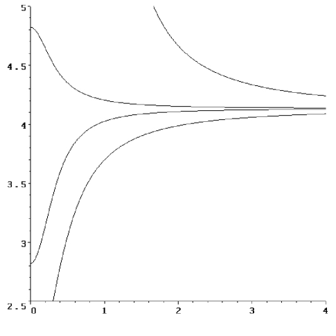
Figure 1: The abscissa is r and the ordinate is $\mathcal{C}_{1}$. Top down the curves show $\rho^{{}^{\prime}}=0$, $p=0$, $\rho=0$ and $p^{{}^{\prime}}=0$. The curves $p=0$ and $\rho=0$ intersect the ordinate at $2+\sqrt{2\pi e}\;\texttt{erf}(\frac{1}{\sqrt{2}})$ and $\sqrt{2\pi e}\;\texttt{erf}(\frac{1}{\sqrt{2}})$ respectively. They are both asymptotic to $\mathcal{C}_{1}=\sqrt{2\pi e}$.

Throughout the physically acceptable distributions $\rho$ and $p$ are monotone decreasing and the adiabatic sound speed $v_{s}$ is subluminal. Some properties are shown in FIG. 2.

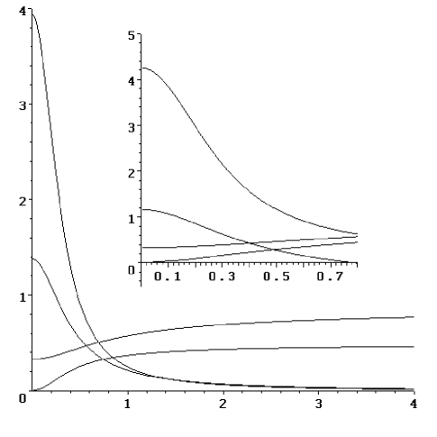
Figure 2: Some internal properties of the solutions. Top down at the origin the curves give $\rho/2$, $p$, $v_{s}$ and $2\tilde{M}/\textrm{r}$ where $v_{s}$ is the adiabatic sound speed and $\tilde{M}$ the effective gravitational mass. The main image is for asymptotic case $\mathcal{C}_{1}=\sqrt{2\pi e}$ and the insert is for $\mathcal{C}_{1}=4.24$ which terminates at $p=0$ where $\textrm{r}\simeq 0.7914$.

We record here in explicit form the essential physical elements of the solutions: The effective gravitational mass is given by

$$\tilde{M}=\frac{\textrm{r}}{2}\left(\frac{\mathcal{F}-1}{\mathcal{F}}\right)$$ (22)

with $\mathcal{F}$ given by (15), the energy density is given by

$$8\pi\;\rho={\frac{2\mathcal{K}\textrm{r}^{2}\left(\mathcal{C}_{1}-\sqrt{2\pi e}\;\mathcal{E}\right)-3\,\mathcal{L}}{4\mathcal{J}^{5}\textrm{r}^{2}}}$$ (23)

where

$$\mathcal{K}\equiv 3\mathcal{J}^{6}+8\mathcal{J}^{4}-5\mathcal{J}^{2}+6$$ (24)

and

$$\mathcal{L}\equiv(\mathcal{J}^{2}+2)(\mathcal{J}-1)^{2}(\mathcal{J}+1)^{2}\mathcal{J},$$ (25)

and the isotropic pressure is given by

$$8\pi\;p=\frac{2\mathcal{P}\textrm{r}^{2}\left(\sqrt{2\pi e}\;\mathcal{E}-\mathcal{C}_{1}\right)+\mathcal{Q}}{4\mathcal{J}^{3}\textrm{r}^{2}}$$ (26)

where

$$\mathcal{P}\equiv(3\mathcal{J}^{2}-1)(\mathcal{J}^{2}+1)$$ (27)

and

$$\mathcal{Q}\equiv(3\mathcal{J}^{2}+1)(\mathcal{J}-1)(\mathcal{J}+1)\mathcal{J}.$$ (28)

Finally, the square of the adiabatic sound speed is given by

$$v_{s}^{2}=\mathcal{J}^{2}\frac{2\mathcal{R}\textrm{r}^{2}\left(\sqrt{2\pi e}\;\mathcal{E}-\mathcal{C}_{1}\right)+\mathcal{S}}{2\mathcal{T}\textrm{r}^{2}\left(\mathcal{C}_{1}-\sqrt{2\pi e}\;\mathcal{E}\right)+\mathcal{U}}$$ (29)

where

$$\mathcal{R}\equiv(\mathcal{J}^{2}-3)(\mathcal{J}-1)(\mathcal{J}+1)\mathcal{J},$$ (30)

$$\mathcal{S}\equiv 3\mathcal{J}^{4}-2\mathcal{J}^{2}+3,$$ (31)

$$\mathcal{T}\equiv(\mathcal{J}^{4}-\mathcal{J}^{2}+6)(\mathcal{J}-1)(\mathcal{J}+1)\mathcal{J},$$ (32)

and

$$\mathcal{U}\equiv-3\mathcal{J}^{6}+8\mathcal{J}^{4}-15\mathcal{J}^{2}+30.$$ (33)

IV Discussion

The Einstein static Universe has been transformed into a class of physically acceptable static fluid spheres whose physical properties have been written out in explicit form. The technique is but a coordinate transformation of one discussed previously lake but it allows a clear understanding how various spacetimes can be interrelated others .