Lattice susceptibility for 2D Hubbard Model within dual fermion method

Abstract

In this paper, we present details of the dual fermion (DF) method to study the non-local correction to single site DMFT. The DMFT two-particle Green’s function is calculated using continuous time quantum monte carlo (CT-QMC) method. The momentum dependence of the vertex function is analyzed and its renormalization based on the Bethe-Salpeter equation is performed in particle-hole channel. We found a magnetic instability in both the dual and the lattice fermions. The lattice fermion susceptibility is calculated at finite temperature in this method and also in another recently proposed method, namely dynamical vertex approximation (D$\Gamma$A). The comparison between these two methods are presented in both weak and strong coupling region. Compared to the susceptibility from quantum monte carlo (QMC) simulation, both of them gave satisfied results.

I Introduction

Strongly correlated electron systems, such as heavy fermion compounds, high-temperature superconductors, have gained much attention from both theoretical and experimental point of view. The competition between the kinetic energy and strong Coulomb interaction of fermions generates a lot of fascinating phenomena. Various theoretical approaches have been developed to treat the regime of intermediate coupling. The widely used perturbative methods, such as random phase approximation (RPA), fluctuation exchange (FLEX)Bickers et al. (1989); Bickers and White (1991a), and the two-particle self-consistent (TPSC)Allen and Tremblay (1995); Vilk et al. (1994) method are based on the expansion in the Coulomb interaction which is only valid in weak-coupling. To go beyond the perturbative approximation and to gain insight of the correlation effects of the fermion systems, new theoretical methods are needed. Dynamical mean field theory (DMFT)Metzner and Vollhardt (1989); Hartmann (1984); George et al. (1996) is a big step forward in the understanding Metal-Insulator transition.

Dynamical mean field theory maps a many-body interacting system on a lattice onto a single impurity embedded in a non-interacting bath. Such a mapping becomes exact in the limit of infinite coordination number. All local temporal fluctuations are taken into account in this theory, however spatial fluctuations are treated on the mean field level. DMFT has been proven a successful theory describing the basic physics of the Mott-Hubbard transition. But the non-local correlation effect can’t always be omitted. Although, straight forward extensions of DMFTHettler et al. (1998); Kotliar et al. (2001); Okamoto et al. (2003); Potthoff (2003); Maier et al. (2005) have captured the influence of short-range correlation, these methods are still not capable of describing the collective behavior, e.g. spin wave excitations of many-body system. At the same time, most of the numerically exact impurity solvers require a substantial amount of time to achieve a desired accuracy even on a small cluster, which makes the investigation of larger lattice to be impossible.

Recently, some efforts have been made to take the spatial fluctuations into account in different waysToschi et al. (2007); Rubtsov et al. ; Kusunose (2006); Tokar and Monnier ; Slezak et al. . All these methods construct the non-local contribution of DMFT from the local two-particle vertex. The electron self-energy is expressed as a function of the two-particle vertex and the single-particle propagator. The cluster extention of DMFT considers the correlation within the small cluster. Compared to these, the diagrammatic re-summation technique involved in these new methods makes them only approximately include the non-local corrections. While, long range correlations are also considered in these methods and the computational burden is not serious.

In this paper we will apply the method of RubtsovRubtsov et al. to consider the vertex renormalization of the DF through the Bethe-Salpeter equation. Lattice susceptibility is calculated from the renormalized DF vertex.

The paper is organized as follows: In Sec. II we summarize the basic idea of the DF method and give details of the calculation. The DMFT two-particle Green’s function and the corresponding vertex calculation are implemented in CT-QMC in Sec. III. The frequency dependent vertex is modified through the Bethe-Salpeter Equation to obtain the momentum dependence in Sec. IV. In Sec. V we present the calculation of the lattice susceptibility and compare it with QMC results and also the works from ToschiToschi et al. (2007). The conclusions are summarized in Sec. VI, where we also present possible application.

II The DF method

We study the general one-band Hubbard model at two dimensions

$$H=\sum_{k,\sigma}\epsilon_{k,\sigma}c_{k\sigma}^{\dagger}c_{k\sigma}^{\phantom{\dagger}}+U\sum_{i}n_{i\uparrow}n_{i\downarrow}$$ (1)

$c_{k\sigma}^{\dagger}(c_{k\sigma})$ creates (annihilates) an electron with spin-$\sigma$ and momentum $k$. The dispersion relation is $\epsilon_{k}=-2t\sum_{i=1}^{N}\cos k_{i}$, where $N$ is the number of lattice sites. The basic idea of the DF methodRubtsov et al. is to transform the hopping between different sites into coupling to an auxiliary field $f(f^{\dagger})$. By doing so, each lattice site can be viewed as an isolated impurity. The interacting lattice problem is reduced to solving a multi-impurity problem which couples to the auxiliary field. This can be done using the standard DMFT calculation. After integrating out the lattice fermions $c(c^{\dagger})$ one can obtain an effective theory of the auxiliary field where DMFT serves as an starting point of the expansion over the coupling between each impurity site with the auxiliary field.

To explicitly demonstrate the above idea we start from the action of DMFT which can be written as

$$S[c^{+},c]=\sum_{i}S_{imp}^{i}-\sum_{\nu,k,\sigma}(\Delta_{\nu}-\epsilon_{k\nu})c_{\nu k\sigma}^{\dagger}c_{\nu k\sigma}^{\phantom{\dagger}}$$ (2)

where $\Delta_{\nu}$ is the hybridization function of the impurity problem defined by $S_{imp}^{i}$ which is the action of an isolated impurity at site $i$ with the local Green’s function $g_{\nu}$. Using the Gaussian identity, we decouple the lattice sites into many impurities which couple only to the field $f$

$$S[c^{\dagger},c;f^{\dagger},f] = \sum_{i}S_{imp}^{i}+\sum_{k,\nu,\sigma}[g_{\nu}^{-1}(c_{k\nu\sigma}^{\dagger}f_{k\nu\sigma}^{\phantom{\dagger}}+h.c.)$$ (3)

$$\hskip 28.45274pt+g_{\nu}^{-2}(\Delta_{\nu}-\epsilon_{k})^{-1}f_{k\nu\sigma}^{\dagger}f_{k\nu\sigma}^{\phantom{\dagger}}]$$

The equivalence of Eqs. (2) and (3) form an exact relation between the Green’s funtion of the lattice electrons and the DF.

$$G_{\nu,k}=g_{\nu}^{-2}(\Delta_{\nu}-\epsilon_{k})^{-2}G_{\nu,k}^{d}+(\Delta_{\nu}-\epsilon_{k})^{-1}$$ (4)

This relation is easily derived by considering the derivative over $\epsilon_{k}$ in the two actions. Eq. (4) allows now to solve the many-body “lattice” problem based on DMFT which is different from the straight forward cluster extension. The problem is now to solve the Green’s function of the DF $G^{d}_{\nu,k}$. It is determined by integrating Eq. (3) over $c^{\dagger}$ and $c$ yielding a Taylor expansion series in powers of $f^{\dagger}$ and $f$. The Grassmann integral ensures that $\bar{f}$ and $f$ appear only in pairs associated with the lattice fermion n-particle vertex obtained from the single-site DMFT calculation. In this paper we restrict our considerations to the two-particle vertex $\gamma^{(4)}$.

Figure 1: The first two self-energy diagrams. They are composed of the local vertices function and DF propagator.

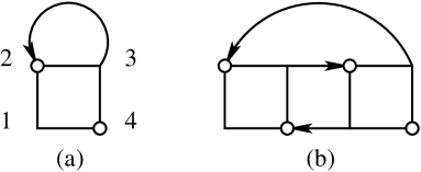
Expanding the Luttinger-Ward functional in $\gamma^{4}$, the first two contributions to the self energy function are the diagrams shown in Fig. 1. Diagram (a) vanishes for the bare DF since this diagram exactly corresponds to the DMFT self consistency. Therefore the first non-local contribution is given by diagram (b). The self-energy for these two diagrams are

$$\Sigma^{(1)}_{\sigma}(k_{1}) =-\frac{T}{N}\sum_{\sigma^{\prime},k_{2}}G_{\sigma^{\prime}}^{d}(k_{2})\gamma^{(4)}_{\sigma\sigma^{\prime}}(\nu,\nu^{\prime};\nu^{\prime},\nu)$$ (5a)

$$\Sigma^{(2)}_{\sigma}(k_{1}) =-\frac{T^{2}}{2N^{2}}\sum_{2,3,4}G^{d}_{\sigma_{2}}(k_{2})G^{d}_{\sigma_{3}}(k_{3})G^{d}_{\sigma_{4}}(k_{4})$$

$$\gamma^{(4)}_{\sigma_{1234}}(\nu_{1},\nu_{2};\nu_{3},\nu_{4})\gamma^{(4)}_{\sigma_{4321}}(\nu_{4},\nu_{3};\nu_{2},\nu_{1})$$

$$\delta_{k_{1}+k_{2},k_{3}+k_{4}}\delta_{\sigma_{1}+\sigma_{2},\sigma_{3}+\sigma_{4}}$$ (5b)

Here space-time notation is used, $k=(\vec{k},\nu)$, $q=(\vec{q},\omega)$. Fermionic Matsubara frequency is $\nu_{n}=(2n+1)\pi/\beta$, bosonic frequency is $\omega_{m}=2m\pi/\beta$ where $\beta$ is the inverse temperature. Together with the bare DF Green’s function $G^{d}_{0}(k)=-g_{\nu}^{2}/[(\Delta_{\nu}-\epsilon_{k})^{-1}+g_{\nu}]$, the new Green’s function can be derived from the Dyson equation

$$[G^{d}(k)]^{-1}=[G_{0}^{d}(k)]^{-1}-\Sigma^{d}(k)$$ (6)

The algorithm of the whole calculation is:

1. Set initial value of $\Delta_{\nu}$ for the first DMFT loop.

2. Determine the single-site DMFT Green’s function $g_{\nu}$ from the hybridization function $\Delta_{\nu}$. The self-consistency condition ensures that the first diagram of the DF self-energy is very small.

3. Go through the DMFT loop once again to calculate the two-particle Green’s function and corresponding $\gamma$-function. The method for determining the $\gamma$-function is implemented for both strong and weak-coupling CT-QMC in the next section of this paper.

4. Start an inner loop calculation to determine the DF Green’s function and in the end the lattice Green’s function.

   1. From Eqs. (5a), (5b) and the Dyson equation (6) to calculate the self-energy of the DF.

   2. Repeatly use Eq. (5a), (5b) and Eq. (6) until the convergence of the DF Green’s function is achived.

   3. The lattice Green’s function is then given by Eq. (4) from that of the DF.

5. Fourier transform the momentum lattice Green’s function into real space. And from the on-site component $G_{ii}$ to determine a new hybridization function $\Delta_{\nu}$ which is given by Eq. (9).

6. Go back to the Step 3. and iteratively perform the outer loop until the hybridization $\Delta_{\nu}$ doesn’t change any more.

Although diagram (a) is exactly zero for the bare DF Green’s function, it gives non-zero contribution from the second loop where the DF Green’s function is updated from Eq. (6). As a result, the hybridization function should also be updated before the next DMFT loop is performed . This is simply done by setting the local full DF Green’s function to zero, together with the condition that the old hybrization function forces the bare local DF Green’s function to be zero ($\sum_{k}G^{0,d}_{\nu,k}=0$), we obtain a set of equations

$$\frac{1}{N}\sum_{k}[G_{\nu,k}-(\Delta^{New}_{\nu}-\epsilon_{k})^{-1}]g_{\nu}^{2}(\Delta^{New}_{\nu}-\epsilon_{k})^{2}=0$$ (7a)

$$\frac{1}{N}\sum_{k}[G^{0}_{\nu,k}-(\Delta^{Old}_{\nu}-\epsilon_{k})^{-1}]g_{\nu}^{2}(\Delta^{Old}_{\nu}-\epsilon_{k})^{2}=0$$ (7b)

which yields

$$\Delta_{\nu}^{New}-\Delta_{\nu}^{Old}\approx\frac{1}{N}\sum_{k}(G_{\nu,k}-G^{0}_{\nu,k})(\Delta^{Old}_{\nu}-\epsilon_{k})^{2}$$ (8)

This equation finally gives us the relation between the new and old hybridization function.

$$\Delta_{\nu}^{New}=\Delta_{\nu}^{Old}+g_{\nu}^{2}G_{loc}^{d}$$ (9)

In the whole calculation, the DF perturbation calculation converges quickly. The most time consuming part of this method is the DMFT calculation of the two particle Green’s function. There are some useful symmetries to accelerate the calculation. As already pointed outAbrikosov et al. (1963); Nozieres (1964), it is convenient to take the symmetric form of the interaction term. The two particle Green’s function is then a fully antisymmetric function. Such fully antisymmetric form is very useful to speed up the calculation of the two particle Green’s function. One does not need to calculate all the frequency points within the cutoff in Mastsubara space, a few special points are calculated and the values for the other points are given by that of those special points through antisymmetric property. In the DF self energy calculation, we always have the convolution type of momentum summation which is very easy to be calculated by fast fourier transform (FFT).

III CT-QMC and two-particle vertex

From the above analysis, the key idea of the DF method is to construct the nonlocal contribution from the auxiliary field and the DMFT two-particle Green’s function. Therefore it is quite important to accurately determine the two-particle vertex. Here we adapt the newly developed CT-QMC methodRubtsov et al. (2005); Werner et al. (2006); Werner and Millis (2006) to calculate the two particle Green’s function $\chi$.

First we briefly outline the CT-QMC technique. For more details, we refer the readers toRubtsov et al. (2005); Werner et al. (2006); Werner and Millis (2006). Here we discuss the two-particle Green’s function and some numerical implemetations in more detailed. Two variants of the CT-QMC methods have been proposed based on the diagrammatic expansion. Unlike the Hirsch-Fye method, these methods don’t have a Trotter error and can approach the low temperature region easily. In the weak-coupling methodRubtsov et al. (2005) the non-interacting part of the partition function is kept and expanded the interaction term into Taylor series. Wick’s theorem ensures that the corresponding expansion can be written into a determinant at each order

$${\cal Z}=\sum_{k}\frac{(-U)^{k}}{k!}\int d\tau_{1}\cdots d\tau_{k}e^{-S_{0}}\det[D_{\uparrow}D_{\downarrow}]$$ (10)

with

$$D_{\uparrow}D_{\downarrow}=\left(\begin{array}[]{cc}\cdots&G_{\uparrow}(\tau_{1}-\tau_{k})\cr\cdots&\cdots\end{array}\right)\left(\begin{array}[]{cc}\cdots&\cdots\cr G_{\downarrow}(\tau_{k}-\tau_{1})&\cdots\end{array}\right)$$ (11)

where $S_{0}$ is the non-interacting action and $G^{0}$ is the Weiss field, and the one-particle Green’s function is measused as

$$G(\nu)=G^{0}(\nu)-\frac{1}{\beta}G^{0}(\nu)\sum_{i,j}M_{i,j}e^{i\nu(\tau_{i}-\tau_{j})}G^{0}(\nu)$$ (12)

In the strong coupling method the effective action is expanded in the hybridization function by integrating over the non-interacting bath degrees of freedom. Such an expansion also yields a determinant.

$${\cal Z}=TrT_{\tau}e^{-S_{loc}}\prod_{\sigma}\sum_{k_{\sigma}}\frac{1}{k_{\sigma}!}\int d\tau_{1}^{s}\cdots d\tau_{k_{\sigma}}^{s}\int d\tau_{1}^{e}\cdots d\tau_{k_{\sigma}}^{e}$$

$$\Psi_{\sigma}(\tau^{e})\left(\begin{array}[]{ccc}\Delta(\tau_{1}^{e}-\tau_{1}^{s})&\cdots&\Delta(\tau_{1}^{e}-\tau_{k_{\sigma}}^{s})\\ \cdots&\ddots&\cdots\\ \Delta(\tau_{k_{\sigma}}^{e}-\tau_{1}^{s})&\cdots&\Delta(\tau_{k_{\sigma}}^{e}-\tau_{k_{\sigma}}^{s})\end{array}\right)\Psi_{\sigma}^{\dagger}(\tau^{s})$$ (16)

Here $\Psi(\tau)=(c_{1}(\tau),c_{2}(\tau),\cdots,c_{k_{\sigma}(\tau)})$. The action is evaluated by a Monte Carlo random walk in the space of expansion order $k$. Therefore the corresponding hybridization matrix changes in every Monte Carlo step. One particle Green’s function is measured from the expansion of hybridization function as $G(\tau_{j}^{e}-\tau_{i}^{s})=M_{i,j}$. $M$ is the inverse matrix of the hybridization function. Apparently one needs to calculate this inverse matrix in every update step which is time consuming, fortunately it can be obtained by the fast-update algorithmRubtsov et al. (2005).

At the same time such a relation allows direct measurement of the Matsubara Green’s function

$$G(i\nu_{n})=\frac{1}{\beta}\sum_{i,j}e^{-i\nu_{n}\tau_{i}^{s}}M_{i,j}e^{i\nu_{n}\tau_{j}^{e}}$$ (17)

Compared with the imaginary time measurement, it seems additional computational time is needed for the sum over every matrix elements $M_{i,j}$. K. Haule proposed to implement such measurement in every fast update procedure which makes sure that only linear amount of time is neededHaule and Kotliar (2007).

In our calculation the Green’s function is measured in the weak-coupling CT-QMC at each accepted update which greatly reduces the computational time. The weak-coupling CT-QMC normally yields a higher perturbation order $k$ than the strong-coupling CT-QMC. It seems that the performance of the strong-coupling CT-QMC is betterGull et al. (2007). Concerning the convergence speed, the weak-coupling CT-QMC is almost same as the strong-coupling one under the above implementation together with a proper choice of $\alpha$, since in strong-coupling CT-QMC more Monte Carlo steps are needed usually in order to smooth the noise of Green’s function at imaginary time around $\beta/2$ or at large Matsubara frequency points. Furthermore, the weak-coupling CT-QMC is much easier implemented for large cluster DMFT calculation, in which case the strong-coupling method needs to handle a big eigenspace. In this paper we mainly use weak-coupling CT-QMC as impurity solver, while all the results can be obtained in the strong-coupling CT-QMC which was used as an accuracy check.

Similarly, we adapt K. Haule’s implementation to calculate the two-particle Green’s function in frequency space. In the weak coupling CT-QMC, the non-interacting action has Gaussian form which ensures the applicability of Wick’s theorem for measuring the two particle Green’s function

$$\chi_{\sigma\sigma^{\prime}}(\nu_{1},\nu_{2},\nu_{3},\nu_{4}) = T[\overline{G_{\sigma}(\nu_{1},\nu_{2})G_{\sigma^{\prime}}(\nu_{3},\nu_{4})}$$ (18)

$$- \delta_{\sigma\sigma^{\prime}}\overline{G_{\sigma}(\nu_{1},\nu_{4})G_{\sigma}(\nu_{3},\nu_{2})}]$$

The over-line indicates the Monte Carlo average. In each Monte Carlo measurement, $G(\nu,\nu^{\prime})$ depends on two different argument $\nu$ and $\nu^{\prime}$, only in the average level, $\overline{G(\nu,\nu^{\prime})}=G(\nu)\delta_{\nu,\nu^{\prime}}$ is a function of single frequency. In each fast-update procedure, the new and old $G(\nu,\nu^{\prime})$ have a closed relation which ensures that one can determine the updated Green’s function $G^{New}(\nu,\nu^{\prime})$ from the old one $G^{Old}(\nu,\nu^{\prime})$. For example, adding pair of kinks and supposing before updating the perturbation order is $k$, then it is $k+1$ for the new M-matrix. The new inserted pair is at $k+1$ row and $k+1$ column.

$$G^{New}(\nu,\nu^{\prime})-G^{old}(\nu,\nu^{\prime})$$ (19)

$$= \frac{M^{New}_{k+1,k+1}}{\beta}G^{0}(\nu)\left\{XL\cdot XR-XR\cdot e^{-i\nu\tau_{k+1}^{s}}\right.$$

$$\left.\hskip 14.22636pt-XL\cdot e^{i\nu^{\prime}\tau_{k+1}^{e}}+e^{-i\nu\tau_{k+1}^{s}+i\nu^{\prime}\tau_{k+1}^{e}}\right\}G^{0}(\nu^{\prime})$$

Here, $XL=\sum_{i=1}^{k}e^{-i\nu\tau_{i}^{s}}L_{i}$, $XR=\sum_{j=1}^{k}e^{i\nu^{\prime}\tau_{j}^{e}}R_{j}$ and $L_{i},R_{j}$ have the same definition as in RefRubtsov et al. (2005). In every step, one only needs to calculates the Green’s function when the update is accepted and only a few calculations are needed. A similar procedure for removing pairs, shiftting end-point operation can be used. Such method is also applicable in the segment picture of strong-coupling CT-QMC. In the weak-coupling CT-QMC, such an implementation greatly improves the calculating speed in low temperature and strong interaction regime. Once one obtains the two frequency dependent Green’s function in every monte carlo step, the two-particle Green’s function can be determined easily from Eq. (18). The two-particle vertex is then given from the following equation:

$$\gamma^{\sigma\sigma^{\prime}}_{\omega}(\nu,\nu^{\prime})=\frac{\beta^{2}[\chi^{\sigma\sigma^{\prime}}_{\omega}(\nu,\nu^{\prime})-\chi^{0}_{\omega}(\nu,\nu^{\prime})]}{g_{\sigma}(\nu)g_{\sigma}(\nu+\omega)g_{\sigma^{\prime}}(\nu^{\prime}+\omega)g_{\sigma^{\prime}}(\nu^{\prime})}$$ (20)

where

$$\chi^{0}_{\omega}(\nu,\nu^{\prime})=T[\delta_{\omega,0}g_{\sigma}(\nu)g_{\sigma^{\prime}}(\nu^{\prime})-\delta_{\sigma\sigma^{\prime}}\delta_{\nu,\nu^{\prime}}g_{\sigma}(\nu)g_{\sigma}(\nu+\omega)]$$ (21)

is the bare susceptibility. For the multi-particle Green’s function, it still can be constructed from the two frequency dependent Green’s function $G(\nu,\nu^{\prime})$, but more terms appear from Wicks theorem. Simply, when set $\nu=\nu^{\prime}$ one can calculate the one-particle Green’s funtion easily.

IV Momentum dependece of Vertex

As mentioned earlier diagram (a) in Fig. 1 only gives the local contribution. The first non-local correction in the DF method is from diagram (b). Momentum dependences comes into this theory through the bubble-like diagram between the two vertices which yields the momentum dependence of the DF vertex. The natural way to renormalize vertex is through the Bethe-Salpeter equation. Since the DMFT vertex is only a function of Matsubara frequency, the integral over internal momentum $k$ and $k^{\prime}$ ensures that the full vertex only depends on the center of mass momentum $Q$. The Bethe-Salpeter equation in the particle-hole channelAbrikosov et al. (1963); Nozieres (1964) are shown in Fig. 2.

From the construction of the DF method, we know the interaction of the DF is coming from the two particle vertex of lattice fermion which is obtained through DMFT calculation. In the Bethe-Salpeter equation, it plays the role of the building-block. The corresponding Bethe-Salpeter equation for these two channels are

$$\Gamma^{ph0,\sigma\sigma^{\prime}}_{Q}(\nu,\nu^{\prime})=\gamma^{\sigma\sigma^{\prime}}_{\omega}(\nu,\nu^{\prime})-$$

$$\frac{T}{N}\sum_{k^{\prime\prime}\sigma^{\prime\prime}}\gamma^{\sigma\sigma^{\prime\prime}}_{\omega}(\nu,\nu^{\prime\prime})G^{d}(k^{\prime\prime})G^{d}(k^{\prime\prime}+Q)\Gamma^{ph0,\sigma^{\prime\prime}\sigma^{\prime}}_{Q}(\nu^{\prime\prime},\nu^{\prime})$$ (22a)

$$\Gamma^{ph1,\sigma\bar{\sigma}}_{Q}(\nu,\nu^{\prime})=\gamma^{\sigma\bar{\sigma}}_{\omega}(\nu,\nu^{\prime})-$$

$$\frac{T}{N}\sum_{k^{\prime\prime}}\gamma^{\sigma\bar{\sigma}}_{\omega}(\nu,\nu^{\prime\prime})G^{d}(k^{\prime\prime})G^{d}(k^{\prime\prime}+Q)\Gamma^{ph1,\sigma\bar{\sigma}}_{Q}(\nu^{\prime\prime},\nu^{\prime})$$ (22b)

Here, the short hand notation of spin configuration is used. $\gamma^{\sigma\sigma^{\prime}}$ represents $\gamma^{\sigma\sigma\sigma^{\prime}\sigma^{\prime}}$, while $\gamma^{\sigma\bar{\sigma}\bar{\sigma}\sigma}$ is denoted by $\gamma^{\sigma\bar{\sigma}}$ where $\bar{\sigma}=-\sigma$. $\Gamma^{ph0(ph1)}$ are the full vertices in the $S_{z}=0$ and $S_{z}=\pm 1$ channel, respectively. $G^{d}$ is the full DF Green’s function obtained from section II which is kept unchanged in the calculation of the Bethe-Salpeter Equation. Different from the work of S. BrenerBrener et al. , we solve the above equations directly in momentum space with the advantage that in this way we can calculate the susceptibility for any specific center of mass momentum $Q$ and it’s convenient to use FFT for investigating larger lattice.

Figure 2: $S_{z}=0$ (ph0) and $S_{z}=\pm 1$ (ph1) particle-hole channels of the DF vertex, between vertices there are two full DF Green’s function. The $S_{z}=\pm 1$ component is the triplet channel, while that for $S_{z}=0$ can be either singlet or triplet.

In Eq. (22) one has to sum over the internal spin indices in the $S_{z}=0$ channel which is not present in $S_{z}=\pm 1$ channel. One can decouple the $S_{z}=0$ channel into the charge and spin channels $\gamma_{c(s)}=\gamma^{\sigma\sigma}\pm\gamma^{\sigma\bar{\sigma}}$ which can be solved seperately, and it turns out that the spin channel vertex function is exactly same as the that in $S_{z}=\pm 1$ channel, see e.g. P. NozieresNozieres (1964). Such relation is true for the DMFT vertex, and was also verified for the momentum dependent vertex in the DF methodBrener et al. . In our calculation, we have solved the $S_{z}=0$ channel by decoupling it to the charge and spin channel, while the $ph1$ channel is not used.

Once the converged momentum dependent DF vertex is obtained, one can determine the corresponding DF susceptibility in the standard way by attaching four Green’s functions to the DF vertex.

$$\chi^{\sigma\sigma^{\prime}}_{d}(Q)=\chi^{0}_{d}(Q)+$$

$$\frac{T^{2}}{N^{2}}\sum_{k,k^{\prime}}G^{d}_{\sigma}(k)G^{d}_{\sigma}(k+Q)\Gamma^{\sigma\sigma^{\prime}}(Q)G^{d}_{\sigma^{\prime}}(k^{\prime})G^{d}_{\sigma^{\prime}}(k^{\prime}+Q)$$ (23a)

$$\chi^{\sigma\bar{\sigma}}_{d}(Q)=\chi^{0}_{d}(Q)+$$

$$\frac{T^{2}}{N^{2}}\sum_{k,k^{\prime}}G^{d}_{\sigma}(k)G^{d}_{\bar{\sigma}}(k+Q)\Gamma^{\sigma\bar{\sigma}}(Q)G^{d}_{\sigma}(k^{\prime})G^{d}_{\bar{\sigma}}(k^{\prime}+Q)$$ (23b)

The momentum sum over $\vec{k}$ and $\vec{k}^{\prime}$ can be performed independently by FFT becasue the DF vertx $\Gamma^{\sigma\sigma^{\prime}}(Q)$ only depends on the center of mass momentum $Q$.

Now the z-component DF spin susceptibility $\langle S^{z}\cdot S^{z}\rangle=\frac{1}{2}(\chi^{\uparrow\uparrow}_{d}-\chi^{\uparrow\downarrow}_{d})$ can be determined from the spin channel component calculated above. In Fig. 3, $\tilde{\chi}^{zz}=\chi^{zz}-\chi_{0}^{zz}$ is shown for $U/t=4$ at temperatures $\beta t=4.0$ (left panel) and $\beta t=1.0$ (right panel). With the lowing down of temperature the DF susceptibility grows up, especially at wave vector $(\pi,\pi)$. The momentum $\vec{k}_{x}$ and $\vec{k}_{y}$ run from $0$ to $2\pi$.

Figure 3: The nontrivial part of the DF spin susceptibilities as a function of momentum in 2D Hubbard Model at $U/t=4.0$, $\beta t=1.0$ (right panel) and $\beta t=4.0$ (left panel). Here 32 $\times$ 32 momentum points are used in the first Brillouin zone.

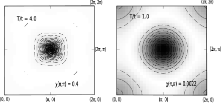
The susceptibility is strongly peaked at the wave vector $(\pi,\pi)$ at the low temperature case and the peak value becomes higher and higher. The magnetic instability of the DF system is indicated by the enhancement of the DF susceptiblity. The effect of momentum dependence of vertex is clearly visible in this diagram. The bare vertex which is only a function of frequency becomes momentum dependent through the Bethe-Salpeter equation. Later on we will see that such momentum dependent vertex plays a very important role in the calculation of the lattice fermion susceptibility.

V Lattice susceptibility

The strong antiferromagnetic fluctuation in 2D system is indicated by the enhancement of the DF susceptibility at the wave vector $(\pi,\pi)$ shown in Fig 3. This is the consequence of the deep relation between the the Green’s function of the lattice and the DF, see Eq. (4). In order to observe the magnetic instability of the lattice fermion directly, we have calculated the lattice susceptibility based on the DF method. By differentiating the partition function in Eqns. (2, 3) twice over the kinetic energy, we obtain an exact relation between the susceptibility of DF and lattice fermions. After some simplificationsBrener et al. , it is given by

$$\chi_{f}(Q)=\chi^{0}_{f}(Q)+$$

$$\frac{T^{2}}{N^{2}}\sum_{k,k^{\prime}}G^{\prime}(k)G^{\prime}(k+Q)\Gamma^{d}_{Q}(\nu,\nu^{\prime})G^{\prime}(k^{\prime})G^{\prime}(k^{\prime}+Q)$$ (24)

Here $G^{\prime}$ cannt be interpreted as a particle propagator, it is defined as:

$$G^{\prime}(k)=\frac{G^{d}(k)}{g_{\nu}[\Delta_{\nu}-\epsilon(k)]}$$ (25)

Again, the sum is performed over internal momentum and frequency $k,k^{\prime}$ which is performed by FFT and rough summing over a few Matsubara points. Again as in Eq. (4), this equation established a connection between the lattice susceptibility and the DF susceptibility. From this point of view, it is easy to understand that the instability of DFs generates the instability of the lattice fermions.

One can also find relations for the higher order Green’s function of the DF and the lattice fermions in the same way. This emphasizes the similar nature of the DF and lattice fermions except that DF possess only non-local information, since the DMFT self-consistency ensures that the local DF Green’s function is exactly zero.

The lattice magnetic susceptibility is calculated using the following definition

$$\chi_{m}(q) = \frac{1}{N}\sum_{i}e^{iq\cdot r_{i}}\int_{0}^{\beta}d\tau e^{-i\omega_{m}\tau}\chi_{f}(i,\tau)$$ (26)

$$= 2(\chi_{f}^{\uparrow\uparrow}-\chi_{f}^{\uparrow\downarrow})$$

where $\chi_{f}(i,\tau)=\langle[n_{i,\uparrow}(\tau)-n_{i,\downarrow}(\tau)]\times[n_{0,\uparrow}(0)-n_{0,\downarrow}(0)]\rangle$. $\chi_{f}$ represents the lattice susceptibility in order to distinguish with that of the DF.

Figure 4: The uniform spin suscetibility of the DF using the bare vertex (only frequency dependent) and the full vertex(vertex from the Bethe-Salpeter quqation) for half filled 2D Hubbard model at $U/t=4.0$ and various temperatures. These results reproduce the similiar solution in comparison with the calculation of finite size of QMC.

We have used two different ways to calculate the lattice susceptibility. First we have solved the above equation using the bare vertex $\Gamma(\nu,\nu^{\prime};\omega)$ which is obtained from the DMFT calculation. In contrast, the second calculation was performed using the full DF vertex. In both of these calculations, the full one particle DF Green’s function was used. The momentum dependent of the DF vertex is obtained through the calculation of the Bethe-Salpeter equation. The lattice susceptibility is expected to be improved if we use the momentum dependence DF vertex. In this way, we can understand the effect of momentum dependence in the DF vertex.

In Fig. 4 we plotted the results for the uniform susceptibility $\chi_{m=0}(0,0)$ by using both the bare and full DF vertex. The lattice QMC resultMoreo (1993) is shown for comparison. The calculation is done for $U/t=4.0$ and several values of temperature. The momentum sum is approximated over 32 $\times$ 32 points here. Both of these calculations reproduce the well known Curie-Weiss law behavior. Surprisingly enough, the results for the bare vertex fit the QMC results better than that for the momentum dependent vertex. We believe that this is the finite size effect of QMCMoreo (1993). A. Moreo showed that $\chi$ becomes smaller when increasing the cluster size $N$. The 4 $\times$ 4 cluster calculation result at the same temperature located above of that from 8 $\times$ 8 cluster calculation. Therefore the results obtained from the full vertex is expected to be more reliable.

Figure 5: Uniform spin susceptibility at the wave vector $(\pi,\pi)$. The QMC results are obtained from Ref.Bickers and White (1991b).

The importance of the momentum dependence of the DF vertex is more clearly observed in the calculation of $\chi_{m}(\pi,\pi)$, see Fig. 5. Again, in this diagram QMC resultsBickers and White (1991b) are shown for comparison. The same parameters are used as in Fig. 4. The result from the DF with bare vertex does not produce the same results compared with QMC solution. Evenmore interesting, with decreasing temperature the deviation becomes larger. On the other hand, the momentum dependent vertex in the DF method gives a satisfactory answer. This shows the importance of the momentum dependence in the DF vertex function. Fig. 6 shows the evolution of $\chi$ against $q$ for fixed transfer frequency $\omega_{m}=0$. The path in momentum space is shown in the inset. From this diagram we can see that $\chi(q,0)$ reaches its maximum value at wave vector $(\pi,\pi)$.

The comparison between the DF and QMC results shows the good performance of DF method. The DF calculation started from a single site DMFT calculation and by introducing an auxiliary field, the non-local information is introduced and nicely reproduces the QMC results. Our calculation could be done within four hours for each value of the temperature on average. In this sense, this method is cheap and reliable compared with the more computationally intensive lattice QMC calculation.

Figure 6: $\chi(q,0)$ vs $q$ at $\beta t=2.0$, $U/t=4.0$ for various $q$ which is along the trajectory shown in the inset.

Similar as the DF method, Dynamical Vertex Approximation (D$\Gamma$A)Toschi et al. (2007) is also based on the two particle local vertex. It deals with the lattice fermion directly, without introducing any auxiliary field. The perturbative nature of this method ensures its validity at weak-coupling regime. Unlike in the DF method, D$\Gamma$A takes the irreducible two particle local vertex as building blocks.

$$\gamma_{c(s)}^{-1}(\nu,\nu^{\prime};\omega)=\gamma^{-1}_{c(s),ir}(\nu,\nu^{\prime};\omega)-\chi_{0}(\nu;\omega)\delta_{\nu,\nu^{\prime}}$$ (27a)

$$\Gamma_{c(s)}^{-1}(\nu,\nu^{\prime};Q)=\gamma^{-1}_{c(s),ir}(\nu,\nu^{\prime};\omega)-\chi_{0}(\nu;Q)\delta_{\nu,\nu^{\prime}}$$ (27b)

with the spin and charge vertex defined as $\gamma_{c(s)}=\gamma^{\uparrow\uparrow}\pm\gamma^{\uparrow\downarrow}$. The bare susceptibility is defined as

$$\chi_{0}(\nu;\omega)=-TG_{loc}(\nu)G_{loc}(\nu+\omega)$$ (28a)

$$\chi_{0}(\nu,Q)=-\frac{T}{N}\sum_{\vec{k}}G^{0}(\vec{k},\nu)G^{0}(\vec{k}+\vec{q},\nu+\omega)$$ (28b)

And the self-energy is calculated through the standard Schwinger-Dyson equation

$$\Sigma(k)=-U\frac{T^{2}}{N^{2}}\sum_{k^{\prime},Q}\Gamma_{f}(k,k^{\prime};Q)G^{0}(k^{\prime})G^{0}(k^{\prime}+Q)G^{0}(k+Q)$$ (29)

Here, the full vertex $\Gamma_{f}(k,k^{\prime};Q)$ is obtained by summing all the channel dependent vertices and subtracting the double counted diagrams.

$$\Gamma_{f}(k,k^{\prime};Q) = \frac{1}{2}\bigg{\{}[3\Gamma_{c}(\nu,\nu^{\prime};Q)-\Gamma_{s}(\nu,\nu^{\prime};Q)]$$ (30)

$$-[\Gamma_{c}(\nu,\nu^{\prime};\omega)-\Gamma_{s}(\nu,\nu^{\prime};\omega)]\bigg{\}}$$

The one particle propagator is given by the DMFT lattice Green’s function where the self energy is purely local $G^{0}(k)=1/[i\nu-\epsilon(k)-\Sigma(\nu)]$, the local Green’s function is $G_{loc}(\nu)=1/[i\nu-\Delta(\nu)-\Sigma(\nu)]$. Then the Dyson equation gives the lattice Green’s function from the self-energy function $G^{-1}=G^{-1}_{0}-\Sigma$.

Figure 7: Comparison with the D$\Gamma$A susceptibilities $\chi(0,0)$ which obtained from both the DMFT lattice Green’s function (D$\Gamma$A $(G^{0}$)) and the full Green’s function (D$\Gamma$A $(G$)), see context for more details.

Before presenting the comparison, we take a deeper look at the analysis of Eq. (27),

$$\Gamma_{c(s)}^{-1}(\nu,\nu^{\prime};Q) = \gamma^{-1}_{c(s)}(\nu,\nu^{\prime};\omega)-$$ (31)

$$[\chi_{0}(\nu;Q)-\chi_{0}(\nu,\omega)]\delta_{\nu,\nu^{\prime}}$$

The second term in the brackets on RHS removes the local term from the bare susceptibility. The whole term in the brackets then represents only the non-local bare susceptibility. In order to compare with the DF method, we take the inverse form of Eq. (22)

$$\Gamma_{d,c{s}}^{-1}(\nu,\nu^{\prime};Q) = \gamma_{c(s)}^{-1}(\nu,\nu^{\prime},\omega)-$$ (32)

$$\frac{T}{N}\sum_{\vec{k}}G^{d}(k)G^{d}(k+q)$$

The above two equations are same except for the last term. Since the local DF Green’s function $G^{d}_{loc}$ is zero, the bare DF susceptibility is purely non-local which coincides with the analysis of D$\Gamma$A Bethe-Salpeter equation. Therefore, it is not surprising that these two methods generate similar results. It is not easy to perform a term to term comparison between the DF method and D$\Gamma$A although the bare susceptibilities have no local term in both of these method. The one particle Green’s functions have different meaning in these two methods.

Figure 8: D$\Gamma$A susceptibilities $\chi(\pi,\pi)$ at $U/t=4.0$. The susceptibility are determined from both of the DMFT and full lattice Green’s function together with the vertex obtained from Eq. (30)

.

The lattice susceptibility within the D$\Gamma$A method is obtained by attaching four Green’s functions on the vertex obtained in Eq. (30). There are two possible choices of the lattice Green’s function, one is the DMFT lattice Green’s function $G^{0}$, the other one is the Green’s function $G$ constructed by the non-local self-energy from the Dyson equation. In Fig. 7 and 8, we presented the D$\Gamma$A lattice susceptibility calculated from both the DMFT lattice Green’s function labeled as D$\Gamma$A($G^{0}$) and the full Green’s function labeled as D$\Gamma$A($G$). The DF result from the calculation with the full DF vertex is re-plotted for comparison. In Fig. 7, the D$\Gamma$A susceptibility calculated from the DMFT Green’s function (D$\Gamma$A($G^{0}$)) is basically the same as the DF susceptibility only with some small deviation. The results for $T/t>1.0$ which are not shown here which nicely repeat the DF and QMC results, the deviation between the D$\Gamma$A and the DF method becomes smaller with the increasing of temperature. The D$\Gamma$A susceptibility is calculated from the full Green’s function (D$\Gamma$A($G$)) shows a different behavior at low temperature regime which reached its maximum value at $T/t\approx 0.36$. As we know, the Hubbard Model at half filling with strong coupling maps to the Heisenberg model, $\chi$ reasches a maximum at $T\approx J$ where $J$ is the effective spin coupling constant given as $4t^{2}/U$. The calculation uses the parameter $U/t=4.0$ which is in the intermediate coupling regime. Therefore we further calculated the lattice susceptibility at $U/t=10.0$ which are shown in Fig. 9.

Figure 9: The comparison of the DF resulsts and that of QMC for the uniform susceptibility at $U/t=10$. 4$\times$4 QMC resultsMoreo (1993) also shows the errorbars.

When the temperature is greater than 0.4, the DF method and D$\Gamma$A (D$\Gamma$A($G^{0}$)) generate the similar results to the QMC calculation. Reducing the temperature further, the QMC susceptibility greatly drops and shows a peak around 0.4 which coincides with the behavior of the Heisenberg model. The DF femion and D$\Gamma$A susceptibility continuously grows up with the decreasing of temperature. Although the D$\Gamma$A with the full Green’s function (D$\Gamma$A($G$)) shows a peak, it locates at $T/t=0.6667$ which is larger than the peak position of the QMC. And D$\Gamma$A($G$) generated a large deviation from that of QMC. In this diagram, we only show the results of the DF approach for $T/t>0.3$ and the D$\Gamma$A results for $T/t>0.4$. The Bethe-salpeter equation of the D$\Gamma$A have a eigenvalue approaching one when further lowering the temperature, which makes the access of lower temperature region impossible.

Figure 10: The evolution of maximum eigenvalue in spin channel against temperature for DF method and D$\Gamma$A.

Fig. 8 shows the results of D$\Gamma$A susceptibilities at wave vector $(\pi,\pi)$. In contrast to the comparison for $\chi(0,0)$ results, the D$\Gamma$A susceptibility calculated from the full Green’s function D$\Gamma$A ($G$) yields better results than that from the calculation with the DMFT Green’s function D$\Gamma$A ($G^{0}$). D$\Gamma$A ($G$) results are almost on top of the DF results, the results with DMFT Green’s function D$\Gamma$A ($G^{0}$) is large than the DF results. The deviation becomes larger at lower temperature. Summarizing, the D$\Gamma$A calculation using the full Green’s function generated the same result as the DF method for $\chi(\pi,\pi)$ while failed to produce $\chi(0,0)$ correctly. In contrast, the calculation with the DMFT Green’s function in D$\Gamma$A nicely produced the results calculated with the DF method for $\chi(0,0)$ while generated larger devivation for $\chi(\pi,\pi)$ at lower temperature regime compared to that from the DF method. Together with Fig. 4 and 5, we can see that the DF fermion calculation with the full DF vertex generated basically the same results for both $\chi(0,0)$ and $\chi(\pi,\pi)$ compared to the results of QMC.

Figure 11: Uniform magentic susceptibility is plotted as a function of dopping at $\beta t=2.5$ and $U/t=4.0,10.0$.

In both the DF method and the D$\Gamma$A, the operation of inverting large matrices is required for solving the Bethe-Salpeter equation. Fig. 10 shows the leading eigenvalue of Eqns. (22) and (27). As expected, the leading eigenvalue approaches one with decreasing temperature which directly indicates the magnetic instability of 2D system. The eigenvalues corresponding to the DF fermion method always lies below of that from D$\Gamma$A indicating the better convergence of the DF method. When the leading eigenvalues are closed to one, the matrix inversion in Eqns. (22) and (27) are ill defined, which prevents the investigation at very low temperature.

Concerning the performance of the DF method, we also calculated the uniform susceptibility at away half-filling. In the strong-coupling limit, the Hubbard model is equivalent to the Heisenberg model with coupling constant $J=4t^{2}/U$. The consequence of doping is to effectively decrease the coupling $J$, which yields the increasing behavior of $\chi$ with doping. The finite size QMC calulationMoreo (1993); Chen and Tremblay (1993) observed a slightly increasing $\chi$ with very small doping at strong interaction or in the low temperature region. Here, we did a similar calculation at $\beta t=2.5$ and $U/t=4,10$. Since the DF method and the D$\Gamma$A do not suffer from the finite size problem. We would expect to observe results similar to those of QMCMoreo (1993); Chen and Tremblay (1993). In D$\Gamma$A the suseceptibility is calculated from the DMFT Green’s function $G^{0}$ and the vertex obtained from Eq. (30). As shown in Fig. 11 at $U/t=4.0$, the susceptibility $\chi$ slightly increases in the weak dopping region where $\delta$ is around $0.05$, DF fermion results clearly showed such behavior, D$\Gamma$A also gave a signal of it. Further doping the system, both the D$\Gamma$A and the DF method reproduce the decrease with doping as already seen in the QMC. With the increasing of interaction, we would expect to see the enhancement of this effect, however our calculation indicates that such increasing-decreasing behaviro dissappear. Both the D$\Gamma$A and the DF method give the same decreasing curve which contradict to QMC resultMoreo (1993). The results will most likely be further improved by including the higher order vertex or calculating the cluster DMFT plus DF/D$\Gamma$AHafermann et al. (2007).

VI Conclusion

In this paper, we extended both the DF method and D$\Gamma$A to calculate the lattice susceptibility. Both of these methods gave equally good results compared with QMC calculation at $U/t=4.0$. Although they are supposed to be weak-coupling methods, at $U/t=10.0$ these two methods generated right results at high temperature region. While both of them failed to reproduce the Heisenberg physics at low temperature. The investigation of the lattice susceptibility suffers from hard determined matrix inversion problem at low temperature regime. The DF methods always generates smaller eigenvalues compared to D$\Gamma$A indicating the better convergence. The implementation of DF method in momentum space greatly improves the calculational speed and makes it easier to deal with larger size lattice.