Generalized SURE for Exponential Families: Applications to Regularization

Abstract

Stein’s unbiased risk estimate (SURE) was proposed by Stein for the independent, identically distributed (iid) Gaussian model in order to derive estimates that dominate least-squares (LS). In recent years, the SURE criterion has been employed in a variety of denoising problems for choosing regularization parameters that minimize an estimate of the mean-squared error (MSE). However, its use has been limited to the iid case which precludes many important applications. In this paper we begin by deriving a SURE counterpart for general, not necessarily iid distributions from the exponential family. This enables extending the SURE design technique to a much broader class of problems. Based on this generalization we suggest a new method for choosing regularization parameters in penalized LS estimators. We then demonstrate its superior performance over the conventional generalized cross validation approach and the discrepancy method in the context of image deblurring and deconvolution. The SURE technique can also be used to design estimates without predefining their structure. However, allowing for too many free parameters impairs the performance of the resulting estimates. To address this inherent tradeoff we propose a regularized SURE objective. Based on this design criterion, we derive a wavelet denoising strategy that is similar in sprit to the standard soft-threshold approach but can lead to improved MSE performance.

I Introduction

Estimation in multivariate problems is a fundamental topic in statistical signal processing. One of the most common recovery strategies for deterministic unknown parameters is the well-known maximum likelihood (ML) method. The ML estimator enjoys several appealing properties, including asymptotic efficiency under suitable regularity conditions. Nonetheless, its mean-squared error (MSE) can be improved upon in the non-asymptotic regime in many different settings.

In their seminal work, Stein and James showed that for the independent, identically-distributed (iid) linear Gaussian model, it is possible to construct a nonlinear estimator with lower MSE than that of ML for all values of the unknowns [1, 2]. Various modifications of the James-Stein method have since been developed that are applicable to the non-iid Gaussian case as well [3, 4, 5, 6, 7, 8].

The James-Stein approach is based on the Stein unbiased risk estimate (SURE) [9, 10], which is an unbiased estimate of the MSE. Since the MSE in general depends on the true unknown parameter values it cannot be used as a design objective. However, using the SURE principle leads to a relatively simple technique for determining methods that have lower MSE than ML. The idea is to choose a class of estimates, and then select the member from the class that minimizes the SURE estimate of the MSE. This strategy has been applied to a variety of different denoising techniques [11, 12, 13, 14]. Typically, in these problems, implicit prior information on the signal to be recovered is incorporated into the chosen structure of the estimate. For example, in wavelet denoising the signal is assumed to be sparse in the wavelet domain which motives the use of thresholding. Only the value of the threshold is determined by the SURE principle.

The SURE method is appealing as it allows to directly approximate the MSE of an estimate from the data, without requiring knowledge of the true parameter values. However, it has two main drawbacks which severely limit its use in practical applications. The first restriction is that it was originally limited to the iid Gaussian case. Several extensions have been developed for different independent models. In particular, a SURE principle for iid, infinitely divisible random variables with finite variance is derived in [15]. Extensions to independent variables from a continuous exponential family are treated in [16, 17], while the discrete exponential case is discussed in [18]. All of these generalizations are confined to the independent case which precludes a variety of important applications such as image deblurring.

The second drawback of using SURE as a design criterion is that in order to get meaningful estimators the basic structure of the estimate must be determined in advance. If no parametrization is assumed, then there are too many free variables to be optimized, and the SURE method will typically not lead to good MSE behavior.

In this paper we extend the basic SURE principle in two directions, in order to circumvent the two fundamental drawbacks outlined above. First, we generalize SURE to multivariate, possibly non-iid exponential families. In particular, we develop an unbiased estimate of the MSE for a general Gaussian vector model. Exponential probability density functions (pdfs) play an important role in statistics due to the Pitman-Koopman-Darmois theorem [19, 20, 21], which states that among distributions whose domain does not vary with the parameter being estimated, only in exponential families is there a sufficient statistic with bounded dimension as the sample size increases [22]. Furthermore, efficient estimators exist only when the underlying model is exponential. Many known distributions are of the exponential form, such as Gaussian, gamma, chi-square, beta, Dirichlet, Bernoulli, binomial, multinomial, Poisson, and geometric distributions. Our result has important practical value as it extends the applicability of the SURE technique to more general estimation models, and in particular to scenarios in which the observations are dependent. This is the situation, for example, when using overcomplete wavelet transforms, and in image deblurring. In addition, we derive results for the case in which the model is rank-deficient so that the pdf depends only on a projection of the parameter vector.

An immediate application of this extension is to the general linear Gaussian model. In this setup, we seek to estimate a parameter vector $\theta$ from noisy, blurred measurements ${{{\bf x}}}={{\bf H}}\mbox{\boldmath{$\theta$}}+{\bf w}$ where ${\bf w}$ is a Gaussian noise vector and ${{\bf H}}$ may be rank deficient. One of the most popular recovery strategies in this context is the regularized least-squares (LS) method. In this approach, the estimate is designed to minimize a regularized LS objective where typical choices of penalization are weighted $\ell_{2}$ or $\ell_{1}$ norms. An important aspect of this technique, which significantly impacts its performance, is selecting the regularization parameter. A variety of different methods have been proposed for this purpose [24, 25, 26, 27, 28, 29, 30, 31]. When an $\ell_{2}$ norm is used to penalize the LS solution, the resulting estimate is linear and is referred to as Tikhonov regularization. One of the most popular regularization selection methods in this context is generalized cross-validation (GCV) [32]. When an $\ell_{1}$ penalty is used, the resulting estimate is nonlinear so that applying the GCV approach is more complicated. An alternative choice is the discrepancy method in which the parameter is chosen such that the resulting data error is equal to the noise variance.

Here, we suggest an alternative strategy based on our extended SURE criterion. Specifically, we use SURE to evaluate the MSE of the penalized solution for any choice of regularization, and then select the value that minimizes the SURE estimate. This allows SURE-based optimization of a broad class of deblurring and deconvolution methods including both linear and nonlinear techniques. A similar approach was studied in the special case of Tikhonov regularization with white noise in [24, 25, 26]. However, our technique is not limited to an $\ell_{2}$ penalty and can be used with any other penalized LS method. When the estimate is not given explicitly but rather as a solution of an optimization problem we can still employ the SURE strategy by using a Monte-Carlo approach to approximate the derivative of the estimate, which figures in the SURE expression [39]. Using several test images and a deconvolution problem, we demonstrate that this strategy often leads to significant performance improvement over the standard GCV and discrepancy selection criteria in the context of image deblurring and deconvolution.

Finally, to circumvent the need for pre-defining a particular structure when applying SURE, we propose an alternative approach based on regularizing the SURE objective. Specifically, we suggest adding a penalization term to the SURE expression and choosing an estimate that minimizes the regularized function. In this way, we can control the properties of the estimate without having to a-priori assume a specific structure. We then illustrate this strategy in the context of wavelet denoising. Instead of assuming a threshold estimate and choosing the threshold to minimize the SURE criterion, as in [11], we design an estimate that minimizes an $\ell_{1}$ regularized SURE objective. The resulting denoising scheme has the form of a threshold with a particular form of shrinkage, that is different than that obtained when using soft or hard thresholding. To evaluate our method, we compare it with SureShrink of Donoho and Johnstone [11], by repeating the simulations reported in their paper. As we show, the recovery results tend to be better using our technique. Moreover, our approach is general as it is not tailored to a specific problem. We thus believe that using a regularized SURE principle together with the generalized SURE developed here can extend the applicability of SURE-based estimators to a broad class of problems.

The remaining of the paper is organized as follows. In Section II we introduce the basic concept of MSE estimation. An extension of SURE to exponential families is developed in Section III. In Section IV we discuss rank-deficient models in which the pdf of the data depends only on a projection of the unknown parameter vector. We then specialize the results to the linear Gaussian model in Section V. Applications to regularization selection are discussed in Section VI. The regularized SURE criterion, together with an application to wavelet denoising, are developed in Section VII.

II MSE Estimation

We denote vectors by boldface lowercase letters, e.g., ${{{\bf x}}}$, and matrices by boldface uppercase letters e.g., ${\mathbf{A}}$. The $i$th component of a vector ${{{\bf y}}}$ is written as $y_{i}$, and $\hat{(\cdot)}$ is an estimated vector. The identity matrix is written as ${{\bf I}}$, ${\mathbf{A}}^{T}$ is the transpose of ${\mathbf{A}}$, and ${\mathbf{A}}^{\dagger}$ denotes the pseudo-inverse. For a length-$m$ vector function ${{\bf h}}({\mathbf{u}})\in{\mathbb{R}}^{m}$ of ${\mathbf{u}}\in{\mathbb{R}}^{m}$,

$$\operatorname{Tr}\left(\frac{\partial{{\bf h}}({\mathbf{u}})}{\partial{\mathbf{u}}}\right)=\sum_{i=1}^{m}\frac{\partial h_{i}({\mathbf{u}})}{\partial u_{i}}.$$ (1)

We consider the class of problems in which our goal is to estimate a deterministic parameter vector $\theta$ from observations ${{{\bf x}}}$ which are related through a pdf $f({{{\bf x}}};\mbox{\boldmath{$\theta$}})$. We further assume that the pdf belongs to the exponential family of distributions and can be expressed in the form

$$f({{{\bf x}}};\mbox{\boldmath{$\theta$}})=r({{{\bf x}}})\exp\{\mbox{\boldmath{$\theta$}}^{T}\phi({{{\bf x}}})-g(\mbox{\boldmath{$\theta$}})\},$$ (2)

where $r({{{\bf x}}})$ and $\phi({{{\bf x}}})$ are functions of the data only, and $g(\mbox{\boldmath{$\theta$}})$ depends on the unknown parameter $\theta$.

As an example of an application where the model (2) can occur, consider the location problem of estimating a parameter vector $\mbox{\boldmath{$\theta$}}\in{\mathbb{R}}^{m}$ from observations ${{{\bf x}}}\in{\mathbb{R}}^{n}$ related through the linear model:

$${{{\bf x}}}={{\bf H}}\mbox{\boldmath{$\theta$}}+{\bf w},$$ (3)

where ${\bf w}$ is a zero-mean Gaussian random vector with covariance ${\mathbf{C}}\succ 0$. The pdf of ${{{\bf x}}}$ is then given by (2) with

$$r({{{\bf x}}})=\frac{1}{\sqrt{(2\pi)^{n}\det({\mathbf{C}})}}\exp\{-(1/2){{{\bf x}}}^{T}{\mathbf{C}}^{-1}{{{\bf x}}}\};$$

$$\phi({{{\bf x}}})={{\bf H}}^{T}{\mathbf{C}}^{-1}{{{\bf x}}};$$

$$g(\mbox{\boldmath{$\theta$}})=(1/2)\mbox{\boldmath{$\theta$}}^{T}{{\bf H}}^{T}{\mathbf{C}}^{-1}{{\bf H}}\mbox{\boldmath{$\theta$}}.$$ (4)

Other examples of distributions in the exponential family include Poisson with unknown mean, exponential with unknown mean, gamma, and Bernoulli or binomial with unknown success probabilities.

Given the model (2), a sufficient statistic for estimating $\theta$ is given by

$${\mathbf{u}}=\phi({{{\bf x}}}).$$ (5)

Therefore, any reasonable estimate of ${{{\bf x}}}$ will be a function only of ${\mathbf{u}}$. More specifically, from the Rao-Blackwell theorem [33] it follows that if $\hat{\mbox{\boldmath{$\theta$}}}$ is an estimate of $\theta$ which is not a function only of ${\mathbf{u}}$, then the estimate $E\{\hat{\mbox{\boldmath{$\theta$}}}|{\mathbf{u}}\}$ has lesser or equal MSE than that of $\hat{\mbox{\boldmath{$\theta$}}}$, for all $\theta$. Therefore, in the sequel, we only consider methods that depend on the data via ${\mathbf{u}}$.

Let $\hat{\mbox{\boldmath{$\theta$}}}$ be an arbitrary estimate of $\theta$, which we would like to design to minimize the MSE, defined by $E\{\|\hat{\mbox{\boldmath{$\theta$}}}-\mbox{\boldmath{$\theta$}}\|^{2}\}$. In practice, $\hat{\mbox{\boldmath{$\theta$}}}={{\bf h}}({\mathbf{u}})$ where ${{\bf h}}({\mathbf{u}})$ is some function of ${\mathbf{u}}$ that is typically chosen to have a particular structure, parameterized by a vector $\alpha$. For example, ${{\bf h}}({\mathbf{u}})=\alpha{\mathbf{u}}$ where $\alpha$ is a scalar, or $h_{i}({\mathbf{u}})=\psi_{\alpha}(u_{i})$ where

$$\psi_{\alpha}(u)=\mbox{sign}(u)[|u|-\alpha]_{+}$$ (6)

is a soft-threshold with cut-off $\alpha$. Ideally, we would like to select $\alpha$ to minimize the MSE. Since this is impossible, as we show below, instead in the SURE approach $\alpha$ is designed to minimize an unbiased estimate (referred to as the SURE estimate) of the MSE.

We can express the MSE of $\hat{\mbox{\boldmath{$\theta$}}}={{\bf h}}({\mathbf{u}})$ as

$$E\left\{\|\hat{\mbox{\boldmath{$\theta$}}}-\mbox{\boldmath{$\theta$}}\|^{2}\right\}=\|\mbox{\boldmath{$\theta$}}\|^{2}+E\left\{\|{{\bf h}}({\mathbf{u}})\|^{2}\right\}-2E\left\{{{\bf h}}^{T}({\mathbf{u}})\mbox{\boldmath{$\theta$}}\right\}.$$ (7)

In order to minimize the MSE over ${{\bf h}}({\mathbf{u}})$ we need to explicitly evaluate the expression

$$v({{\bf h}},\mbox{\boldmath{$\theta$}})=E\left\{\|{{\bf h}}({\mathbf{u}})\|^{2}\right\}-2E\left\{{{\bf h}}^{T}({\mathbf{u}})\mbox{\boldmath{$\theta$}}\right\}.$$ (8)

Evidently, the MSE will depend in general on $\theta$, which is unknown, and therefore cannot be minimized. Instead, we may seek an unbiased estimate of $v({{\bf h}},\mbox{\boldmath{$\theta$}})$ and then choose ${{\bf h}}$ to minimize this estimate. The difficult expression to approximate is $E\{{{\bf h}}^{T}({\mathbf{u}})\mbox{\boldmath{$\theta$}}\}$ as the dependency on $\theta$ is explicit. Therefore, we concentrate on estimating this term. If this can be done, then we can easily obtain an unbiased MSE estimate. Specifically, suppose we construct a function $g({{\bf h}}({\mathbf{u}}))$ that depends only on ${\mathbf{u}}$ (and not on $\theta$), such that

$$E\left\{g({{\bf h}}({\mathbf{u}}))\right\}=E\left\{{{\bf h}}^{T}({\mathbf{u}})\mbox{\boldmath{$\theta$}}\right\}{\stackrel{{\scriptstyle\triangle}}{{=}}}E_{{{\bf h}},\mbox{\small\boldmath{$\theta$}}}.$$ (9)

Then

$$\hat{v}({{\bf h}})=\|{{\bf h}}({\mathbf{u}})\|^{2}-2g({{\bf h}}({\mathbf{u}})),$$ (10)

is an unbiased estimate of $v({{\bf h}},\mbox{\boldmath{$\theta$}})$, since clearly $E\{\hat{v}({{\bf h}})\}=v({{\bf h}},\mbox{\boldmath{$\theta$}})$. A reasonable strategy therefore is to select ${{\bf h}}({\mathbf{u}})$ to minimize our assessment $\hat{v}({{\bf h}})$ of the MSE. This approach was first proposed by Stein in [9, 10] for the iid Gaussian model (3) with ${\mathbf{C}}={{\bf I}}$ and ${{\bf H}}={{\bf I}}$.

The design framework proposed above reduces to finding an unbiased estimate of $E_{{{\bf h}},\mbox{\small\boldmath{$\theta$}}}$. Clearly, any such approximation will depend on the pdf $f({{{\bf x}}};\mbox{\boldmath{$\theta$}})$. In the next section we develop an unbiased estimate when the pdf is given by the exponential model (2). Before addressing the general setting, to ease the exposition we illustrate the main idea proposed by Stein, by first considering the simpler iid Gaussian case. In this setting we seek to estimate a vector $\mbox{\boldmath{$\theta$}}\in{\mathbb{R}}^{m}$ from measurements ${{{\bf x}}}=\mbox{\boldmath{$\theta$}}+{\bf w}$, where ${\bf w}$ is a zero-mean Gaussian random vector with iid components of variance $\sigma^{2}$. In Section IV we treat the more difficult case in which ${\mathbf{u}}$ lies in a subspace ${\mathcal{A}}$ of ${\mathbb{R}}^{m}$, and the pdf (2) depends on $\theta$ only through its orthogonal projection onto ${\mathcal{A}}$. This situation arises, for example, in the linear Gaussian model (3) when ${{\bf H}}$ is rank deficient. For this setup, we develop a SURE estimate of the MSE in estimating the projected parameter. In Sections V and VI we consider several examples of estimates in which the free parameters are chosen to minimize the SURE objective. In particular, we propose alternatives to the popular GCV and discrepancy methods for regularization. In Section VII, we suggest a regularized SURE strategy for determining ${{\bf h}}({\mathbf{u}})$ without the need for parametrization, and demonstrate its performance in the context of wavelet denoising.

III Extended SURE Principle

III-A IID Gaussian Model

We begin our development by treating the iid Gaussian setting. Since from (II), ${\mathbf{u}}=(1/\sigma^{2}){{{\bf x}}}$, we consider estimates $\hat{\mbox{\boldmath{$\theta$}}}={{\bf h}}({{{\bf x}}})$ that are a function of ${{{\bf x}}}$.

To develop an unbiased estimate of $E_{{{\bf h}},\mbox{\small\boldmath{$\theta$}}}$, we exploit the fact that for the Gaussian pdf $f({{{\bf x}}};\mbox{\boldmath{$\theta$}})$

$$(x_{i}-\theta_{i})f({{{\bf x}}};\mbox{\boldmath{$\theta$}})=-\sigma^{2}\frac{\partial f({{{\bf x}}};\mbox{\boldmath{$\theta$}})}{\partial x_{i}}.$$ (11)

Assuming that $E\{|h_{i}({{{\bf x}}})|\}$ is bounded and $h_{i}({{{\bf x}}})$ is weakly differentiable in ${{{\bf x}}}$, we have that

$$E_{{{\bf h}},\mbox{\small\boldmath{$\theta$}}} = \sum_{i=1}^{m}\int_{-\infty}^{\infty}h_{i}({{{\bf x}}})\theta_{i}f({{{\bf x}}};\mbox{\boldmath{$\theta$}})d{{{\bf x}}}$$ (12)

$$= \sum_{i=1}^{m}\int_{-\infty}^{\infty}h_{i}({{{\bf x}}})\left(x_{i}f({{{\bf x}}};\mbox{\boldmath{$\theta$}})+\sigma^{2}\frac{\partial f({{{\bf x}}};\mbox{\boldmath{$\theta$}})}{\partial x_{i}}\right)d{{{\bf x}}}$$

$$= E\{{{\bf h}}^{T}({{{\bf x}}}){{{\bf x}}}\}+\sigma^{2}\sum_{i=1}^{m}\int_{-\infty}^{\infty}h_{i}({{{\bf x}}})\frac{\partial f({{{\bf x}}};\mbox{\boldmath{$\theta$}})}{\partial x_{i}}d{{{\bf x}}},$$

where the second equality is a result of (11). To evaluate the second term in (12), we use integration by parts:

$$\int_{-\infty}^{\infty}h_{i}({{{\bf x}}})\frac{\partial f({{{\bf x}}};\mbox{\boldmath{$\theta$}})}{\partial x_{i}}d{{{\bf x}}}=-\int_{-\infty}^{\infty}h_{i}^{\prime}({{{\bf x}}})f_{i}({{{\bf x}}};\mbox{\boldmath{$\theta$}})d{{{\bf x}}}=-E\{h_{i}^{\prime}({{{\bf x}}})\},$$ (13)

were we denoted $h_{i}^{\prime}({{{\bf x}}})=\partial h_{i}({{{\bf x}}})/\partial x_{i}$, and used the fact that $|h_{i}({{{\bf x}}})f({{{\bf x}}};\mbox{\boldmath{$\theta$}})|\rightarrow 0$ for $|x_{i}|\rightarrow\infty$ since $E\{|h_{i}({{{\bf x}}})|\}$ is bounded. We conclude from (12) and (13) that

$$E_{{{\bf h}},\mbox{\small\boldmath{$\theta$}}}=-\sigma^{2}\sum_{i=1}^{m}E\{h^{\prime}_{i}({{{\bf x}}})\}+E\{{{\bf h}}^{T}({{{\bf x}}}){{{\bf x}}}\},$$ (14)

and therefore,

$$-\sigma^{2}\sum_{i=1}^{m}\frac{\partial h_{i}({{{\bf x}}})}{\partial x_{i}}+{{\bf h}}^{T}({{{\bf x}}}){{{\bf x}}}$$ (15)

is an unbiased estimate of $E_{{{\bf h}},\mbox{\small\boldmath{$\theta$}}}$.

III-B Extended SURE

We now extend the basic approach outlined in the previous section to the general class of exponential pdfs. In order to address this model, we only consider methods that depend on the data via ${\mathbf{u}}$. This enables the use of integration by parts, similar to the iid Gaussian setting.

The following theorem provides an unbiased estimate of $E\left\{{{\bf h}}^{T}({\mathbf{u}})\mbox{\boldmath{$\theta$}}\right\}$ which depends only on ${\mathbf{u}}$ and not on the unknown parameters $\theta$.

Theorem 1

Let ${{{\bf x}}}$ denote a random vector with exponential pdf given by (2), and let ${\mathbf{u}}=\phi({{{\bf x}}})$ be a sufficient statistic for estimating $\theta$ from ${{{\bf x}}}$. Let ${{\bf h}}({\mathbf{u}})$ be an arbitrary function of $\theta$ that is weakly differentiable in ${\mathbf{u}}$ and such that $E\left\{|h_{i}({\mathbf{u}})|\right\}$ is bounded. Then

$$E\left\{{{\bf h}}^{T}({\mathbf{u}})\mbox{\boldmath{$\theta$}}\right\}=-E\left\{\operatorname{Tr}\left(\frac{\partial{{\bf h}}({\mathbf{u}})}{\partial{\mathbf{u}}}\right)\right\}-E\left\{{{\bf h}}^{T}({\mathbf{u}})\frac{\partial\ln q({\mathbf{u}})}{\partial{\mathbf{u}}}\right\},$$ (16)

where

$$q({\mathbf{u}})=\int r({{{\bf x}}})\delta({\mathbf{u}}-\phi({{{\bf x}}}))d{{{\bf x}}},$$ (17)

and $\delta({{{\bf x}}})$ is the Kronecker delta function.

Note, that as we show in the proof of the theorem, the pdf $f({\mathbf{u}};\mbox{\boldmath{$\theta$}})$ of ${\mathbf{u}}$ is given by

$$f({\mathbf{u}};\mbox{\boldmath{$\theta$}})=q({\mathbf{u}})\exp\{\mbox{\boldmath{$\theta$}}^{T}{\mathbf{u}}-g(\mbox{\boldmath{$\theta$}})\}.$$ (18)

Therefore, an alternative to computing $q({\mathbf{u}})$ using (17) is to evaluate the pdf of ${\mathbf{u}}$ and then use (18).

From the theorem, it follows that

$$-\operatorname{Tr}\left(\frac{\partial{{\bf h}}({\mathbf{u}})}{\partial{\mathbf{u}}}\right)-{{\bf h}}^{T}({\mathbf{u}})\frac{\partial\ln q({\mathbf{u}})}{\partial{\mathbf{u}}}\,$$ (19)

is an unbiased estimate of $E\{{{\bf h}}^{T}({\mathbf{u}})\mbox{\boldmath{$\theta$}}\}$. In the iid Gaussian case, ${\mathbf{u}}=(1/\sigma^{2}){{{\bf x}}}$ so that

$$\frac{\partial{{\bf h}}({\mathbf{u}})}{\partial{\mathbf{u}}}=\sigma^{2}\frac{\partial{{\bf h}}({{{\bf x}}})}{\partial{{{\bf x}}}}.$$ (20)

Furthermore, ${\mathbf{u}}$ is a Gaussian iid vector with elements that have mean $(1/\sigma^{2})\mbox{\boldmath{$\theta$}}$ and variance $1/\sigma^{2}$ so that $q({\mathbf{u}})$, which is the normalization factor, is given by $q({\mathbf{u}})=K\exp\{-\|{\mathbf{u}}\|^{2}\sigma^{2}/2\}$ for a constant $K$. Consequently

$$\frac{\partial\ln q({\mathbf{u}})}{\partial{\mathbf{u}}}=-\sigma^{2}{\mathbf{u}}=-{{{\bf x}}}.$$ (21)

Substituting (20) and (21) into (19), the estimate reduces to (15), derived in the iid Gaussian setting.

Proof:

To prove the theorem we first determine the pdf of ${\mathbf{u}}$. Since ${\mathbf{u}}=\phi({{{\bf x}}})$ we have that [33, p. 127]

$$f({\mathbf{u}};\mbox{\boldmath{$\theta$}})=\int f({{{\bf x}}};\mbox{\boldmath{$\theta$}})\delta({\mathbf{u}}-\phi({{{\bf x}}}))d{{{\bf x}}}.$$ (22)

Substituting (2) into (22),

$$f({\mathbf{u}};\mbox{\boldmath{$\theta$}}) = \exp\{\mbox{\boldmath{$\theta$}}^{T}{\mathbf{u}}-g(\mbox{\boldmath{$\theta$}})\}\int r({{{\bf x}}})\delta({\mathbf{u}}-\phi({{{\bf x}}}))d{{{\bf x}}}$$ (23)

$$= q({\mathbf{u}})\exp\{\mbox{\boldmath{$\theta$}}^{T}{\mathbf{u}}-g(\mbox{\boldmath{$\theta$}})\}.$$

Now,

$$E\left\{{{\bf h}}^{T}({\mathbf{u}})\mbox{\boldmath{$\theta$}}\right\}=$$ (24)

$$= \int{{\bf h}}^{T}({\mathbf{u}})\mbox{\boldmath{$\theta$}}\exp\{\mbox{\boldmath{$\theta$}}^{T}{\mathbf{u}}-g(\mbox{\boldmath{$\theta$}})\}q({\mathbf{u}})d{\mathbf{u}}$$

$$= \sum_{i=1}^{m}\int h_{i}({\mathbf{u}})\theta_{i}\exp\{\mbox{\boldmath{$\theta$}}^{T}{\mathbf{u}}-g(\mbox{\boldmath{$\theta$}})\}q({\mathbf{u}})d{\mathbf{u}}.$$

Noting that

$$\theta_{i}\exp\{\mbox{\boldmath{$\theta$}}^{T}{\mathbf{u}}-g(\mbox{\boldmath{$\theta$}})\}=\frac{\partial\exp\{\mbox{\boldmath{$\theta$}}^{T}{\mathbf{u}}-g(\mbox{\boldmath{$\theta$}})\}}{\partial u_{i}},$$ (25)

we have

$$\int_{-\infty}^{\infty}h_{i}({\mathbf{u}})\theta_{i}\exp\{\mbox{\boldmath{$\theta$}}^{T}{\mathbf{u}}-g(\mbox{\boldmath{$\theta$}})\}q({\mathbf{u}})du_{i}=$$ (26)

$$= \int_{-\infty}^{\infty}h_{i}({\mathbf{u}})q({\mathbf{u}})\frac{\partial\exp\{\mbox{\boldmath{$\theta$}}^{T}{\mathbf{u}}-g(\mbox{\boldmath{$\theta$}})\}}{\partial u_{i}}du_{i}$$

$$= -\int_{-\infty}^{\infty}\frac{\partial h_{i}({\mathbf{u}})q({\mathbf{u}})}{\partial u_{i}}\exp\{\mbox{\boldmath{$\theta$}}^{T}{\mathbf{u}}-g(\mbox{\boldmath{$\theta$}})\}du_{i},$$

where we used the fact that $|h_{i}({\mathbf{u}})q({\mathbf{u}})\exp\{\mbox{\boldmath{$\theta$}}^{T}{\mathbf{u}}-g(\mbox{\boldmath{$\theta$}})\}|\rightarrow 0$ for $|u_{i}|\rightarrow\infty$ since $E\{|h_{i}({\mathbf{u}})|\}$ is bounded. Now,

$$\frac{\partial h_{i}({\mathbf{u}})q({\mathbf{u}})}{\partial u_{i}}=\frac{\partial h_{i}({\mathbf{u}})}{\partial u_{i}}q({\mathbf{u}})+\frac{\partial q({\mathbf{u}})}{\partial u_{i}}h_{i}({\mathbf{u}}).$$ (27)

Substituting (26) and (27) into (24),

$$E\left\{{{\bf h}}^{T}({\mathbf{u}})\mbox{\boldmath{$\theta$}}\right\}=$$ (28)

$$= -\sum_{i=1}^{m}\int\frac{\partial h_{i}({\mathbf{u}})q({\mathbf{u}})}{\partial u_{i}}\exp\{\mbox{\boldmath{$\theta$}}^{T}{\mathbf{u}}-g(\mbox{\boldmath{$\theta$}})\}\partial{\mathbf{u}}$$

$$= \sum_{i=1}^{m}\left(-E\left\{\frac{\partial h_{i}({\mathbf{u}})}{\partial u_{i}}\right\}-E\left\{\frac{\partial q({\mathbf{u}})}{\partial u_{i}}\frac{h_{i}({\mathbf{u}})}{q({\mathbf{u}})}\right\}\right)$$

$$= -E\left\{\operatorname{Tr}\left(\frac{\partial{{\bf h}}({\mathbf{u}})}{\partial{\mathbf{u}}}\right)\right\}-E\left\{{{\bf h}}^{T}({\mathbf{u}})\frac{\partial\ln q({\mathbf{u}})}{\partial{\mathbf{u}}}\right\},$$

which completes the proof of the theorem. ∎

Based on Theorem 1 we can develop a generalized SURE principle for estimating an unknown parameter vector $\theta$ in an exponential model. Specifically, let $\hat{\mbox{\boldmath{$\theta$}}}={{\bf h}}({\mathbf{u}})$ be an arbitrary estimate of $\theta$ based on the data ${{{\bf x}}}$, where ${{\bf h}}({\mathbf{u}})$ satisfies the regularity conditions of Theorem 1. Combining (7) and Theorem 1, an unbiased estimate of the MSE of $\hat{\mbox{\boldmath{$\theta$}}}$ is given by

$$S({{\bf h}})=\|\mbox{\boldmath{$\theta$}}\|^{2}+\|{{\bf h}}({\mathbf{u}})\|^{2}+2\operatorname{Tr}\left(\frac{\partial{{\bf h}}({\mathbf{u}})}{\partial{\mathbf{u}}}\right)+2{{\bf h}}^{T}({\mathbf{u}})\frac{\partial\ln q({\mathbf{u}})}{\partial{\mathbf{u}}}.$$ (29)

We may then design $\hat{\mbox{\boldmath{$\theta$}}}$ by choosing ${{\bf h}}({\mathbf{u}})$ to minimize $S({{\bf h}})$.

In the iid Gaussian case, (29) reduces to

$$\|\mbox{\boldmath{$\theta$}}\|^{2}+\|{{\bf h}}({{{\bf x}}})\|^{2}+2\sigma^{2}\frac{\partial{{\bf h}}({{{\bf x}}})}{\partial{{{\bf x}}}}-2{{\bf h}}^{T}({{{\bf x}}}){{{\bf x}}}$$ (30)

where we used the fact that ${\mathbf{u}}=(1/\sigma^{2}){{{\bf x}}}$ which implies $\partial\ln q({\mathbf{u}})/\partial{\mathbf{u}}=-{{{\bf x}}}$, and $\partial{{\bf h}}({\mathbf{u}})/\partial{\mathbf{u}}=\sigma^{2}\partial{{\bf h}}({{{\bf x}}})/\partial{{{\bf x}}}$. The MSE estimate (30) was first proposed by Stein in [9, 10].

The SURE estimate can be used to determine unknown regularization parameters which comprise a given estimation strategy. An example is the SureShrink approach to wavelet denoising [11]. Extending this technique, our general SURE objective (29) may be used to select regularization parameters in more general models. We discuss these ideas in the context of linear Gaussian problems in Section V.

IV Rank-Deficient Models

In some settings, the sufficient statistic ${\mathbf{u}}$ lies in a subspace ${\mathcal{A}}$ of ${\mathbb{R}}^{m}$. As an example, suppose that in the Gaussian model (3) ${{\bf H}}$ is rank-deficient. In this case ${\mathbf{u}}={{\bf H}}^{T}{\mathbf{C}}^{-1}{{{\bf x}}}$ lies in the range space ${\mathcal{R}}({{\bf H}}^{T})$ of ${{\bf H}}^{T}$, which is a subspace of ${\mathbb{R}}^{m}$. If $\theta$ is not restricted to a subspace, then we do not expect to be able to reliably estimate $\theta$ from ${\mathbf{u}}$, unless some additional information on $\theta$ is known. Nonetheless, we may still obtain a reliable assessment of the part of $\theta$ that lies in ${\mathcal{A}}$. Denote by ${{\bf P}}$ the orthogonal projection onto ${\mathcal{A}}$. Then, we show below, that if ${\mathbf{u}}$ depends on $\theta$ only through ${{\bf P}}\mbox{\boldmath{$\theta$}}$, and in addition ${\mathbf{u}}$ has an exponential pdf, then we can obtain a SURE estimate of the error in ${\mathcal{A}}$, namely $E\{\|{{\bf P}}\hat{\mbox{\boldmath{$\theta$}}}-{{\bf P}}\mbox{\boldmath{$\theta$}}\|^{2}\}$. If in addition $\hat{\mbox{\boldmath{$\theta$}}}$ lies in ${\mathcal{A}}$, then up to a constant, independent of $\hat{\mbox{\boldmath{$\theta$}}}$, this approximation is also an unbiased estimate of the true MSE $E\{\|\hat{\mbox{\boldmath{$\theta$}}}-\mbox{\boldmath{$\theta$}}\|^{2}\}$.

To derive the SURE estimate in this case, we first note that if ${\mathbf{u}}$ lies in ${\mathcal{A}}$, then

$$\mbox{\boldmath{$\theta$}}^{T}{\mathbf{u}}=({{\bf P}}\mbox{\boldmath{$\theta$}})^{T}({{\bf P}}{\mathbf{u}}).$$ (31)

Suppose that ${\mathcal{A}}$ has dimension $r<m$. Since ${{\bf P}}\mbox{\boldmath{$\theta$}}$ lies in an $r$-dimensional space, it can be expressed in terms of $r$ components in an appropriate basis. Denoting by ${\mathbf{V}}$ an $m\times r$ matrix with orthonormal vectors that span ${\mathcal{A}}={\mathcal{R}}({{\bf P}})$, the vector ${{\bf P}}\mbox{\boldmath{$\theta$}}$ can be expressed as ${{\bf P}}\mbox{\boldmath{$\theta$}}={\mathbf{V}}\mbox{\boldmath{$\theta$}}^{\prime}$ for an appropriate length-$r$ vector $\mbox{\boldmath{$\theta$}}^{\prime}$. Similarly, ${{\bf P}}{\mathbf{u}}={\mathbf{V}}{\mathbf{u}}^{\prime}$. Therefore, we can write

$$\mbox{\boldmath{$\theta$}}^{T}{\mathbf{u}}=\mbox{\boldmath{$\theta$}}^{\prime T}{\mathbf{u}}^{\prime},$$ (32)

where we used the fact that ${\mathbf{V}}^{T}{\mathbf{V}}={{\bf I}}$. We assume that ${\mathbf{u}}^{\prime}$ is a sufficient statistic for $\mbox{\boldmath{$\theta$}}^{\prime}$ and that $f({\mathbf{u}}^{\prime};\mbox{\boldmath{$\theta$}}^{\prime})$ has an exponential pdf:

$$f({\mathbf{u}}^{\prime};\mbox{\boldmath{$\theta$}}^{\prime})=q({\mathbf{u}}^{\prime})\exp\{\mbox{\boldmath{$\theta$}}^{\prime T}{\mathbf{u}}^{\prime}-g(\mbox{\boldmath{$\theta$}}^{\prime})\}.$$ (33)

Under this assumption, we next derive a SURE estimate of the MSE in ${\mathcal{A}}$.

The MSE in estimating $\theta$ can then be written as

$$E\{\|\hat{\mbox{\boldmath{$\theta$}}}-\mbox{\boldmath{$\theta$}}\|^{2}\}=E\{\|{{\bf P}}\hat{\mbox{\boldmath{$\theta$}}}-{{\bf P}}\mbox{\boldmath{$\theta$}}\|^{2}\}+E\{\|({{\bf I}}-{{\bf P}})\hat{\mbox{\boldmath{$\theta$}}}-({{\bf I}}-{{\bf P}})\mbox{\boldmath{$\theta$}}\|^{2}\}.$$ (34)

If $\hat{\mbox{\boldmath{$\theta$}}}$ lies in ${\mathcal{A}}$, then $({{\bf I}}-{{\bf P}})\hat{\mbox{\boldmath{$\theta$}}}=0$ and the second term is constant, independent of $\hat{\mbox{\boldmath{$\theta$}}}$. Therefore, in this case, to optimize $\hat{\mbox{\boldmath{$\theta$}}}$ it is sufficient to obtain an unbiased estimate of the first term. As we show below, such an assessment can be derived using similar ideas to those in Theorem 1. Even if $\hat{\mbox{\boldmath{$\theta$}}}$ does not lie in ${\mathcal{A}}$, the SURE estimate we develop may be used to approximate the first term. Since ${\mathbf{u}}$ depends only on ${{\bf P}}\mbox{\boldmath{$\theta$}}$, it is reasonable to restrict attention to estimates $\hat{\mbox{\boldmath{$\theta$}}}={{\bf h}}_{\mbox{\boldmath{$\alpha$}}}({\mathbf{u}})$ where the parameters $\alpha$ are tuned to minimize the MSE in ${\mathcal{A}}$ $E\{\|{{\bf P}}\hat{\mbox{\boldmath{$\theta$}}}-{{\bf P}}\mbox{\boldmath{$\theta$}}\|^{2}\}$, subject to any other prior information we may have, such as norm constraints on $\theta$. In such cases we can use a regularized SURE criterion with the SURE objective being the MSE in ${\mathcal{A}}$, as we discuss in Section VII.

We now develop a SURE estimate of the MSE $E\{\|{{\bf P}}\hat{\mbox{\boldmath{$\theta$}}}-{{\bf P}}\mbox{\boldmath{$\theta$}}\|^{2}\}$. To this end we need to find an unbiased estimate of

$$E\{\hat{\mbox{\boldmath{$\theta$}}}^{T}{{\bf P}}\mbox{\boldmath{$\theta$}}\}=E\{\hat{\mbox{\boldmath{$\theta$}}}^{T}{\mathbf{V}}\mbox{\boldmath{$\theta$}}^{\prime}\}=E\{({\mathbf{V}}^{T}\hat{\mbox{\boldmath{$\theta$}}})^{T}\mbox{\boldmath{$\theta$}}^{\prime}\}$$ (35)

Let $\hat{\mbox{\boldmath{$\theta$}}}={{\bf h}}({\mathbf{u}})={{\bf h}}({\mathbf{u}}^{\prime})$ (since ${\mathbf{u}}={\mathbf{V}}{\mathbf{u}}^{\prime}$, it is clear that $\hat{\mbox{\boldmath{$\theta$}}}$ is a function of ${\mathbf{u}}^{\prime}$). By our assumption, $\mbox{\boldmath{$\theta$}}^{\prime}$ has an exponential pdf with sufficient statistic ${\mathbf{u}}^{\prime}$. Therefore, we can apply Theorem 1 to ${\mathbf{V}}^{T}{{\bf h}}({\mathbf{u}})$ for any function ${{\bf h}}({\mathbf{u}})$ that obeys the conditions of the theorem, which yields

$$E\left\{{{\bf h}}^{T}({\mathbf{u}}){\mathbf{V}}\mbox{\boldmath{$\theta$}}^{\prime}\right\} = -E\left\{\operatorname{Tr}\left({\mathbf{V}}^{T}\frac{\partial{{\bf h}}({\mathbf{u}}^{\prime})}{\partial{\mathbf{u}}^{\prime}}\right)\right\}-E\left\{{{\bf h}}^{T}({\mathbf{u}}^{\prime}){\mathbf{V}}\frac{\partial\ln q({\mathbf{u}}^{\prime})}{\partial{\mathbf{u}}^{\prime}}\right\}$$ (36)

$$= -E\left\{\operatorname{Tr}\left({{\bf P}}\frac{\partial{{\bf h}}({\mathbf{u}})}{\partial{\mathbf{u}}}\right)\right\}-E\left\{{{\bf h}}^{T}({\mathbf{u}}){\mathbf{V}}\frac{\partial\ln q({\mathbf{u}}^{\prime})}{\partial{\mathbf{u}}^{\prime}}\right\},$$

where we used the fact that ${{\bf P}}={\mathbf{V}}{\mathbf{V}}^{T}$ and

$$\frac{\partial{{\bf h}}({\mathbf{u}}^{\prime})}{\partial{\mathbf{u}}^{\prime}}=\frac{\partial{{\bf h}}({\mathbf{u}})}{\partial{\mathbf{u}}}{\mathbf{V}}.$$ (37)

We conclude that if ${{\bf h}}({\mathbf{u}})$ is an estimate of a parameter vector $\theta$, where ${\mathbf{u}}$ lies in a subspace ${\mathcal{A}}$ and is a sufficient statistic for estimating ${{\bf P}}\mbox{\boldmath{$\theta$}}$, with ${{\bf P}}$ denoting the orthogonal projection onto ${\mathcal{A}}$, then an unbiased estimate of the MSE $E\{\|{{\bf P}}{{\bf h}}({\mathbf{u}})-{{\bf P}}\mbox{\boldmath{$\theta$}}\|^{2}\}$ is given by

$$S({{\bf h}})=\|{{\bf P}}\mbox{\boldmath{$\theta$}}\|^{2}+\|{{\bf P}}{{\bf h}}({\mathbf{u}})\|^{2}+2\operatorname{Tr}\left({{\bf P}}\frac{\partial{{\bf h}}({\mathbf{u}})}{\partial{\mathbf{u}}}\right)+2{{\bf h}}^{T}({\mathbf{u}}){\mathbf{V}}\frac{\partial\ln q({\mathbf{u}}^{\prime})}{\partial{\mathbf{u}}^{\prime}},$$ (38)

with ${\mathbf{u}}={\mathbf{V}}{\mathbf{u}}^{\prime}$ and ${\mathbf{V}}$ denoting an orthonormal basis for ${\mathcal{A}}$. When ${\mathcal{A}}={\mathbb{R}}^{m}$, ${{\bf P}}={{\bf I}},{\mathbf{V}}={{\bf I}}$ and (38) reduces to (29).

V Linear Gaussian Model

We now specialize the SURE principle to the linear Gaussian model (3). We begin by treating the case in which ${{\bf H}}$ is an $n\times m$ matrix with $n\geq m$ and full column rank. We then discuss the rank-deficient scenario.

V-A Full-Rank Model

To use Theorem 1 we need to compute the pdf $q({\mathbf{u}})$ of ${\mathbf{u}}$. Since ${\mathbf{u}}={{\bf H}}^{T}{\mathbf{C}}^{-1}{{{\bf x}}}$, it is a Gaussian random vector with mean ${{\bf H}}^{T}{\mathbf{C}}^{-1}{{\bf H}}\mbox{\boldmath{$\theta$}}$ and covariance ${{\bf H}}^{T}{\mathbf{C}}^{-1}{{\bf H}}$. As $q({\mathbf{u}})$ is the function multiplying the exponential in the pdf of ${\mathbf{u}}$, it follows from (II) that

$$q({\mathbf{u}})=K\exp\{-(1/2){\mathbf{u}}^{T}({{\bf H}}^{T}{\mathbf{C}}^{-1}{{\bf H}})^{-1}{\mathbf{u}}\},$$ (39)

where $K$ is a constant, independent of ${\mathbf{u}}$. Therefore,

$$\frac{\partial\ln q({\mathbf{u}})}{\partial{\mathbf{u}}}=-({{\bf H}}^{T}{\mathbf{C}}^{-1}{{\bf H}})^{-1}{\mathbf{u}}=-\hat{\mbox{\boldmath{$\theta$}}}_{\operatorname{ML}},$$ (40)

where $\hat{\mbox{\boldmath{$\theta$}}}_{\operatorname{ML}}$ is the ML estimate of $\theta$ given by

$$\hat{\mbox{\boldmath{$\theta$}}}_{\operatorname{ML}}=({{\bf H}}^{T}{\mathbf{C}}^{-1}{{\bf H}})^{-1}{{\bf H}}^{T}{\mathbf{C}}^{-1}{{{\bf x}}}.$$ (41)

It then follows from Theorem 1 that

$$E\left\{{{\bf h}}^{T}({\mathbf{u}})\mbox{\boldmath{$\theta$}}\right\}=-E\left\{\operatorname{Tr}\left(\frac{\partial{{\bf h}}({\mathbf{u}})}{d{\mathbf{u}}}\right)-{{\bf h}}^{T}({\mathbf{u}})\hat{\mbox{\boldmath{$\theta$}}}_{\operatorname{ML}}\right\}.$$ (42)

Using (29) and (40) we conclude that

$$S({{\bf h}})=\|\mbox{\boldmath{$\theta$}}\|^{2}+\|{{\bf h}}({\mathbf{u}})\|^{2}+2\left(\operatorname{Tr}\left(\frac{\partial{{\bf h}}({\mathbf{u}})}{\partial{\mathbf{u}}}\right)-{{\bf h}}^{T}({\mathbf{u}})\hat{\mbox{\boldmath{$\theta$}}}_{\operatorname{ML}}\right),$$ (43)

is an unbiased estimate of the MSE.

V-B Rank-Deficient Model

Next, we consider the linear Gaussian model (3) with a rank-deficient ${{\bf H}}$.

Suppose that ${{\bf H}}$ has a singular value decomposition ${{\bf H}}={{\bf U}}\Sigma{{\bf Q}}^{T}$ for some unitary matrices ${{\bf U}}$ and ${{\bf Q}}$. Let ${{\bf H}}$ have rank $r$ so that $\Sigma$ is a diagonal $n\times m$ matrix what the first $r$ diagonal elements equal to $\sigma_{i}>0$ and the remaining elements equal $0$. In this case, ${\mathbf{V}}$ is equal to the first $r$ columns of ${{\bf Q}}$ and $\mbox{\boldmath{$\theta$}}^{\prime}={\mathbf{V}}^{T}\mbox{\boldmath{$\theta$}}$. A sufficient statistic for estimating $\mbox{\boldmath{$\theta$}}^{\prime}$ is ${\mathbf{u}}^{\prime}={\mathbf{V}}^{T}{{\bf H}}^{T}{\mathbf{C}}^{-1}{{{\bf x}}}$. Indeed, ${\mathbf{u}}^{\prime}$ is a Gaussian random vector with mean $\mu^{\prime}={\mathbf{V}}^{T}{{\bf H}}^{T}{\mathbf{C}}^{-1}{{\bf H}}\mbox{\boldmath{$\theta$}}$ and covariance ${\mathbf{C}}^{\prime}={\mathbf{V}}^{T}{{\bf H}}^{T}{\mathbf{C}}^{-1}{{\bf H}}{\mathbf{V}}$. Using the SVD of ${{\bf H}}$ we have that

$$\mu^{\prime} = \Lambda[{{\bf U}}^{T}{\mathbf{C}}^{-1}{{\bf U}}]_{r}\mbox{\boldmath{$\theta$}}^{\prime},$$

$${\mathbf{C}}^{\prime} = \Lambda[{{\bf U}}^{T}{\mathbf{C}}^{-1}{{\bf U}}]_{r},$$ (44)

where $\Lambda$ is an $r\times r$ diagonal matrix with diagonal elements $\sigma_{i}^{2}>0$ and $[{\mathbf{A}}]_{r}$ is the $r\times r$ top-left principle block of size $r$ of the matrix ${\mathbf{A}}$. Since ${\mathbf{C}}\succ 0$, ${\mathbf{C}}^{\prime}$ is invertible. Therefore,

$$f({\mathbf{u}}^{\prime};\mbox{\boldmath{$\theta$}}^{\prime})=q({\mathbf{u}}^{\prime})\exp\{\mbox{\boldmath{$\theta$}}^{\prime}{\mathbf{u}}^{\prime}-g(\mbox{\boldmath{$\theta$}}^{\prime})\}$$ (45)

with

$$q({\mathbf{u}}^{\prime})=\frac{1}{\sqrt{(2\pi)^{n}\det({\mathbf{C}}^{\prime})}}\exp\{-(1/2){\mathbf{u}}^{\prime T}{\mathbf{C}}^{\prime-1}{\mathbf{u}}^{\prime}\};$$

$$g(\mbox{\boldmath{$\theta$}}^{\prime})=(1/2)\mbox{\boldmath{$\theta$}}^{\prime T}\Lambda[{{\bf U}}^{T}{\mathbf{C}}^{-1}{{\bf U}}]_{r}\mbox{\boldmath{$\theta$}}^{\prime}.$$ (46)

We therefore conclude from (38) that an unbiased estimate of the MSE $E\{\|{{\bf P}}{{\bf h}}({\mathbf{u}})-{{\bf P}}\mbox{\boldmath{$\theta$}}\|^{2}\}$ is given by

$$\|{{\bf P}}\mbox{\boldmath{$\theta$}}\|^{2}+\|{{\bf P}}{{\bf h}}({\mathbf{u}})\|^{2}+2\left(\operatorname{Tr}\left({{\bf P}}\frac{\partial{{\bf h}}({\mathbf{u}})}{\partial{\mathbf{u}}}\right)-{{\bf h}}^{T}({\mathbf{u}})\hat{\mbox{\boldmath{$\theta$}}}_{\operatorname{ML}}\right),$$ (47)

where $\hat{\mbox{\boldmath{$\theta$}}}_{\operatorname{ML}}=({{\bf H}}^{T}{\mathbf{C}}^{-1}{{\bf H}})^{\dagger}{{\bf H}}^{T}{\mathbf{C}}^{-1}{{{\bf x}}}$ is an ML estimate. Here we used the fact that ${\mathbf{V}}{\mathbf{C}}^{\prime-1}{\mathbf{u}}^{\prime}=({{\bf H}}^{T}{\mathbf{C}}^{-1}{{\bf H}})^{\dagger}{{\bf H}}^{T}{\mathbf{C}}^{-1}{{{\bf x}}}$.

We summarize our results for the linear Gaussian model in the following proposition.

Proposition 1

Let ${{{\bf x}}}$ denote measurements of an unknown parameter vector $\theta$ in the linear Gaussian model (3), where ${\bf w}$ is a zero-mean Gaussian random vector with covariance ${\mathbf{C}}\succ 0$. Let ${{\bf h}}({\mathbf{u}})$ with ${\mathbf{u}}={{\bf H}}^{T}{\mathbf{C}}^{-1}{{{\bf x}}}$ be an arbitrary function of $\theta$ that is weakly differentiable in ${\mathbf{u}}$ and such that $E\left\{|h_{i}({\mathbf{u}})|\right\}$ is bounded, and let ${{\bf P}}$ be an orthogonal projection onto ${\mathcal{R}}({{\bf H}}^{T})$. Then

$$E\left\{{{\bf h}}^{T}({\mathbf{u}}){{\bf P}}\mbox{\boldmath{$\theta$}}\right\}=-E\left\{\operatorname{Tr}\left({{\bf P}}\frac{\partial{{\bf h}}({\mathbf{u}})}{\partial{\mathbf{u}}}\right)-{{\bf h}}^{T}({\mathbf{u}})\hat{\mbox{\boldmath{$\theta$}}}_{\operatorname{ML}}\right\},$$

where

$$\hat{\mbox{\boldmath{$\theta$}}}_{\operatorname{ML}}=({{\bf H}}^{T}{\mathbf{C}}^{-1}{{\bf H}})^{\dagger}{{\bf H}}^{T}{\mathbf{C}}^{-1}{{{\bf x}}}$$

is an ML estimate of $\theta$. An unbiased estimate of the MSE $E\{\|{{\bf P}}{{\bf h}}({\mathbf{u}})-{{\bf P}}\mbox{\boldmath{$\theta$}}\|^{2}\}$ is

$$S({{\bf h}})=\|{{\bf P}}\mbox{\boldmath{$\theta$}}\|^{2}+\|{{\bf P}}{{\bf h}}({\mathbf{u}})\|^{2}+2\left(\operatorname{Tr}\left({{\bf P}}\frac{\partial{{\bf h}}({\mathbf{u}})}{\partial{\mathbf{u}}}\right)-{{\bf h}}^{T}({\mathbf{u}})\hat{\mbox{\boldmath{$\theta$}}}_{\operatorname{ML}}\right).$$ (48)

V-C Examples

To illustrate the use of the SURE principle, suppose that we consider estimators of the form $\hat{\mbox{\boldmath{$\theta$}}}=\alpha\hat{\mbox{\boldmath{$\theta$}}}_{\operatorname{ML}}$ where $\hat{\mbox{\boldmath{$\theta$}}}_{\operatorname{ML}}$ is given by (41), and we would like to select a good choice of $\alpha$. To this end, we minimize the SURE unbiased estimate of the MSE given by Proposition 1 with ${{\bf h}}({\mathbf{u}})=\alpha\hat{\mbox{\boldmath{$\theta$}}}_{\operatorname{ML}}$. Note that in this case ${{\bf h}}({\mathbf{u}})\in{\mathcal{R}}({{\bf H}}^{T})$ so that $S({{\bf h}})+\|({{\bf I}}-{{\bf P}})\mbox{\boldmath{$\theta$}}\|^{2}$ is an unbiased estimate of the total MSE $E\{\|\hat{\mbox{\boldmath{$\theta$}}}-\mbox{\boldmath{$\theta$}}\|^{2}\}$ and therefore it suffices to minimize $S({{\bf h}})$.

For this choice of ${{\bf h}}({\mathbf{u}})$, minimizing $S({{\bf h}})$ is equivalent to minimizing

$$\alpha^{2}\|\hat{\mbox{\boldmath{$\theta$}}}_{\operatorname{ML}}\|^{2}+2\left(\alpha\operatorname{Tr}\left(({{\bf H}}^{T}{\mathbf{C}}^{-1}{{\bf H}})^{\dagger}\right)-\alpha\|\hat{\mbox{\boldmath{$\theta$}}}_{\operatorname{ML}}\|^{2}\right).$$ (49)

The optimal choice of $\alpha$ is

$$\alpha=1-\frac{\operatorname{Tr}\left(({{\bf H}}^{T}{\mathbf{C}}^{-1}{{\bf H}})^{\dagger}\right)}{\|\hat{\mbox{\boldmath{$\theta$}}}_{\operatorname{ML}}\|^{2}},$$ (50)

resulting in

$$\hat{\mbox{\boldmath{$\theta$}}}=\left(1-\frac{\operatorname{Tr}\left(({{\bf H}}^{T}{\mathbf{C}}^{-1}{{\bf H}})^{\dagger}\right)}{\|\hat{\mbox{\boldmath{$\theta$}}}_{\operatorname{ML}}\|^{2}}\right)\hat{\mbox{\boldmath{$\theta$}}}_{\operatorname{ML}}.$$ (51)

The estimate of (51) coincides with the balanced blind minimax method proposed in [7, Eq. (45)], which was derived based on a minimax framework [8]. Here we see that the same technique results from applying our generalized SURE criterion. A striking feature of this estimate, proved in [7], is that when ${{\bf H}}^{T}{\mathbf{C}}^{-1}{{\bf H}}$ is invertible and its effective dimension is larger than $4$, it dominates ML for all values of $\theta$ (see Theorem 3 in [7]). This means that its MSE is always lower than that of the ML method, regardless of the true value of $\theta$.

When ${{\bf H}}={{\bf I}}$ and ${\mathbf{C}}=\sigma^{2}{{\bf I}}$, (51) reduces to

$$\hat{\mbox{\boldmath{$\theta$}}}=\left(1-\frac{n\sigma^{2}}{\|{{{\bf x}}}\|^{2}}\right){{{\bf x}}},$$ (52)

which coincides with Stein’s estimate [1]. This technique is known to dominate ML for $n\geq 3$.

If in addition we require that $\alpha\geq 0$, then the estimate of (51) becomes

$$\hat{\mbox{\boldmath{$\theta$}}}=\left[1-\frac{\operatorname{Tr}\left(({{\bf H}}^{T}{\mathbf{C}}^{-1}{{\bf H}})^{\dagger}\right)}{\|\hat{\mbox{\boldmath{$\theta$}}}_{\operatorname{ML}}\|^{2}}\right]_{+}\hat{\mbox{\boldmath{$\theta$}}}_{\operatorname{ML}},$$ (53)

where we used the notation

$$[x]_{+}=\left\{\begin{array}[]{ll}x,&x\geq 0;\\ 0,&x<0.\end{array}\right.$$ (54)

The method of (53) is a positive-part version of (51). In the iid case, it reduces to the positive-part Stein’s estimate [35], which is known to dominate the standard Stein approach (52).

Next, consider the case in which ${{\bf H}}={{\bf I}}$ and ${\mathbf{C}}={{\bf D}}$ with ${{\bf D}}=\operatorname{diag}\,(\sigma_{1}^{2},\ldots,\sigma_{n}^{2})$ and suppose we seek a diagonal estimate of the form $\hat{\theta}_{i}=\alpha_{i}x_{i}$. Minimizing the unbiased estimate of (48) in this case is equivalent to minimizing

$$\sum_{i=1}^{n}\alpha_{i}^{2}x_{i}^{2}+2\sum_{i=1}^{n}\sigma_{i}^{2}\alpha_{i}-2\sum_{i=1}^{n}\alpha_{i}x_{i}^{2},$$ (55)

which yields

$$\alpha_{i}=1-\frac{\sigma_{i}^{2}}{x_{i}^{2}}.$$ (56)

Restricting the coefficients $\alpha_{i}$ to be non-negative leads to the estimate

$$\hat{\theta}_{i}=\left[1-\frac{\sigma_{i}^{2}}{x_{i}^{2}}\right]_{+}x_{i}.$$ (57)

In contrast to $\hat{\mbox{\boldmath{$\theta$}}}$ of (51), which dominates the ML method, it can be proven that the estimate of (57) is not dominating. Thus, we see that by allowing for too many free parameters, we impair the performance of the SURE-based estimate. On the other hand, assuming strong structure, as in (51), severely restricts the class of estimators and consequently limits the possible performance advantage which can be obtained. In Section VII we suggest a regularized SURE strategy in order to overcome this inherent tradeoff between over-parametrization and performance.

VI Application to Regularization Selection

A popular strategy for solving inverse problems of the form (3) is to use regularization techniques in conjunction with a LS objective. Specifically, the estimate $\hat{\mbox{\boldmath{$\theta$}}}$ is chosen to minimize a regularized LS criterion:

$$({{{\bf x}}}-{{\bf H}}\hat{\mbox{\boldmath{$\theta$}}}){\mathbf{C}}^{-1}({{{\bf x}}}-{{\bf H}}\hat{\mbox{\boldmath{$\theta$}}})+\lambda\|{\mathbf{L}}\hat{\mbox{\boldmath{$\theta$}}}\|$$ (58)

where the norm is arbitrary. Here ${\mathbf{L}}$ is some regularization operator such as the discretization of a first or second order differential operator that accounts for smoothness properties of $\theta$, and $\lambda$ is the regularization parameter [28, 27]. An important problem in practice is the selection of $\lambda$, which strongly effects the recovery performance. One of the most popular approaches to choosing $\lambda$ when the estimate is linear (as is the case when a squared-$\ell_{2}$ norm is used in (58)) is the generalized cross-validation (GCV) method [32]. When the estimate takes on a more complicated nonlinear form, a popular selection method is the discrepancy principle [26].

Based on our generalized SURE criterion, we choose $\lambda$ to minimize the SURE objective (48). As we demonstrate for the cases in which the norm in (58) is the squared-$\ell_{2}$ or $\ell_{1}$ norms, this method can dramatically outperform GCV and the discrepancy technique in practical applications.

VI-A Image Deblurring

We first consider the case in which the squared-$\ell_{2}$ norm is used in (58). The solution then has the form

$$\hat{\mbox{\boldmath{$\theta$}}}=({{\bf Q}}+\lambda{\mathbf{L}}^{T}{\mathbf{L}})^{-1}{{\bf H}}^{T}{\mathbf{C}}^{-1}{{{\bf x}}},$$ (59)

where for brevity we denoted

$${{\bf Q}}={{\bf H}}^{T}{\mathbf{C}}^{-1}{{\bf H}}.$$ (60)

The estimate (59) is commonly referred to as Tikhonov regularization [23].

In the GCV method, $\lambda$ is chosen to minimize

$$G(\lambda)=\frac{1}{\operatorname{Tr}^{2}({{\bf I}}-({{\bf Q}}+\lambda{\mathbf{L}}^{T}{\mathbf{L}})^{-1}{{\bf Q}})}\sum_{i=1}^{n}({{{\bf x}}}_{i}-[{{\bf H}}\hat{\mbox{\boldmath{$\theta$}}}]_{i})^{2}.$$ (61)

The SURE choice follows directly from minimizing (48). In our simulations below, both minimizations where performed by using the fmincon function on Matlab.

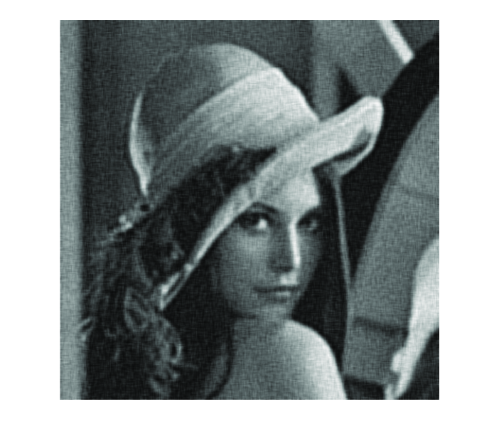
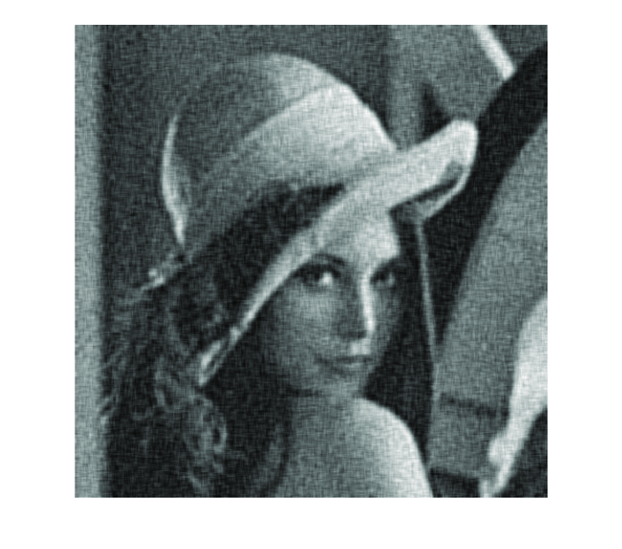
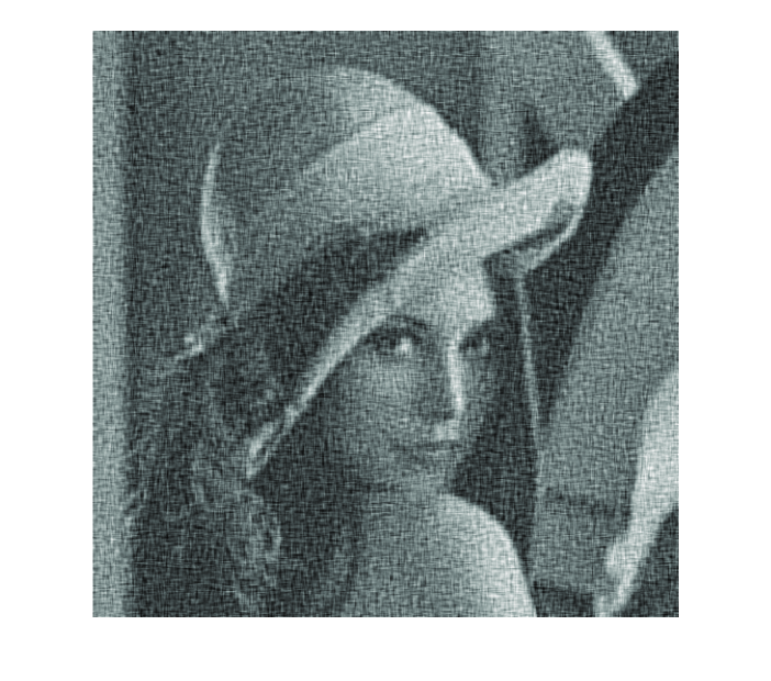
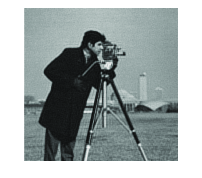
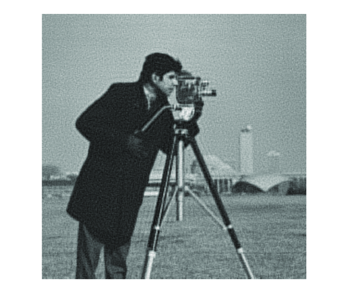
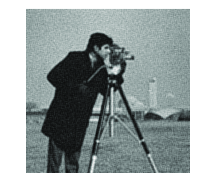
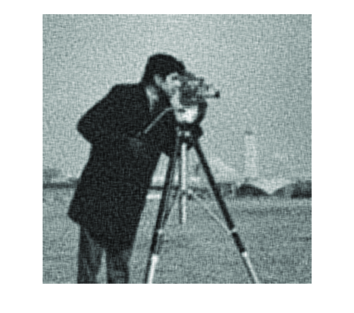
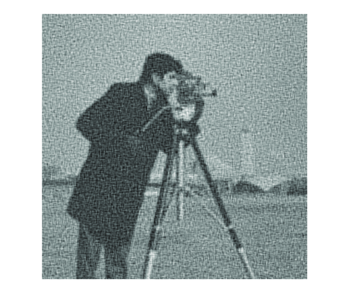
To demonstrate the performance of the proposed regularization method, we tested it in the context of image deblurring using the HNO deblurring package for Matlab based on [36]. We chose several test images, and blurred them using a Gaussian point-spread function of dimension 9 with standard deviation 6 using the function psfGauss. We then added zero-mean, Gaussian white noise with variance $\sigma^{2}$. In Figs. 1 and 2 we compare the deblurred images resulting from using the Tikhonov estimate (59) with ${\mathbf{L}}={{\bf I}}$ where the regularization parameter is chosen according to our new SURE criterion (left) and the GCV method (right), for different noise levels.

(a)                                            (b)

(c)                                            (d)

(e)                                            (f)

Figure 1: Deblurring of Lena using Tikhonov regularization with SURE (left) and GCV (right) choices of regularization and different noise levels: (a), (b) $\sigma=0.01$ (c),(d) $\sigma=0.05$ (e),(f) $\sigma=0.1$.

(a)                                            (b)

(c)                                            (d)

(e)                                            (f)

Figure 2: Deblurring of Cameraman using Tikhonov regularization with SURE (left) and GCV (right) choices of regularization and different noise levels: (a), (b) $\sigma=0.01$ (c),(d) $\sigma=0.05$ (e),(f) $\sigma=0.1$.

As can be seen from the figures, our SURE based approach leads to a substantial performance improvement over the standard GCV criterion. This can also be seen in Tables I and II in which we report the resulting MSE values.

TABLE I: MSE for Tikhonov Deblurring of Lena

	$\sigma=0.01$	$\sigma=0.05$	$\sigma=0.1$
GCV	0.0022	0.0077	0.0133
SURE	0.0011	0.0025	0.0042

TABLE II: MSE for Tikhonov Deblurring of Cameraman

	$\sigma=0.01$	$\sigma=0.05$	$\sigma=0.1$
GCV	0.0033	0.0121	0.0221
SURE	0.0016	0.0039	0.0064

VI-B Deconvolution Example

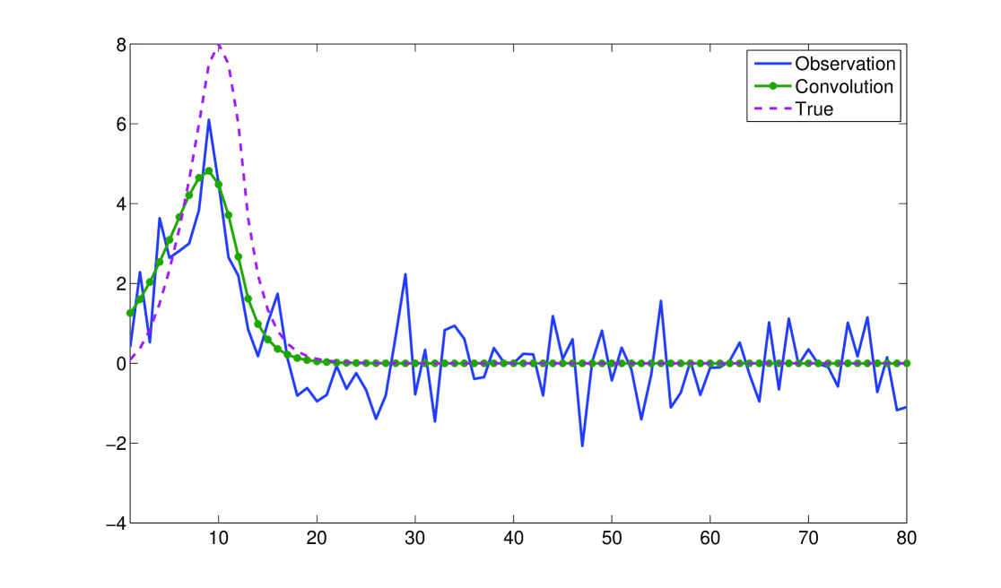
As another application of the SURE, consider the standard deconvolution problem in which a signal $\theta[\ell]$ is convolved by an impulse response $h[\ell]$ and contaminated by additive white Gaussian noise with variance $\sigma^{2}$. The observations $x[\ell]$ can be written in the form of the linear model (3) where ${{{\bf x}}}$ is the vector containing the observations $x[\ell]$, $\theta$ consists of the input signal $\theta[\ell]$, and ${{\bf H}}$ is a Toeplitz matrix, representing convolution with the impulse response $h[\ell]$.

To recover $\theta[\ell]$ we may use a penalized LS approach (58) where we assume that the original signal $\theta[\ell]$ is smooth. This can be accounted for by choosing a penalization of the form $\|{\mathbf{L}}\mbox{\boldmath{$\theta$}}\|_{1}$ where ${\mathbf{L}}$ represents a second order derivative operator. The resulting penalized LS estimate can be determined by solving a quadratic optimization problem. In our simulations, we used CVX, a package for specifying and solving convex programs in Matlab [37].

Since the resulting estimate is non-linear, due to the $\ell_{1}$ penalization, we cannot apply the GCV equation (61). Instead, a popular approach to tune the parameter $\lambda$ is to use the discrepancy principle in which $\lambda$ is chosen such that the residual $\|{{{\bf x}}}-{{\bf H}}\hat{\mbox{\boldmath{$\theta$}}}\|^{2}$ is equal to the noise level $n\sigma^{2}$ [26, 25].

To evaluate the performance of the SURE principle in this context, we consider an example from the Regularization Tools [38] for Matlab. All the problems in this toolbox are discretized versions of the Fredholm integral equation of the first kind:

$$g(s)=\int_{a}^{b}K(s,t)\theta(t)dt$$ (62)

where $K(s,t)$ is the kernel and $\theta(t)$ is the solution for a given $g(s)$. The problem is to estimate $\theta(t)$ from noisy samples of $g(s)$. Using a midpoint rule with $n$ points, (62) reduces to an $n\times n$ linear system ${{{\bf x}}}_{T}={{\bf H}}\mbox{\boldmath{$\theta$}}$. The functions in this toolbox differ in $K(t,s)$ and $\theta(s)$. Below we consider the function heat(n) with $n=80$. The output of the function is the matrix ${{\bf H}}$ and the true vector $\theta$ (which represents $\theta(t)$). The observations are ${{{\bf x}}}={{{\bf x}}}_{T}+{\bf w}$ where ${\bf w}$ is a white Gaussian noise vector with variance $\sigma^{2}=1$.

In Fig. 3 we plot the original signal along with the observations ${{{\bf x}}}$, and the clean convolved signal ${{{\bf x}}}_{T}={{\bf H}}\mbox{\boldmath{$\theta$}}$.

Figure 3: The original signal $\theta$ (dashed), the clean convolved signal (star) and the observations ${{{\bf x}}}$ with $\sigma=1$.

The original signal along with the estimates using the SURE principle and the discrepancy method are plotted in Fig. 4.

Figure 4: Deconvolution using weighted $\ell_{1}$ regularization with the discrepancy principle, SURE (star) and the true signal (dashed) with $\sigma=1$.

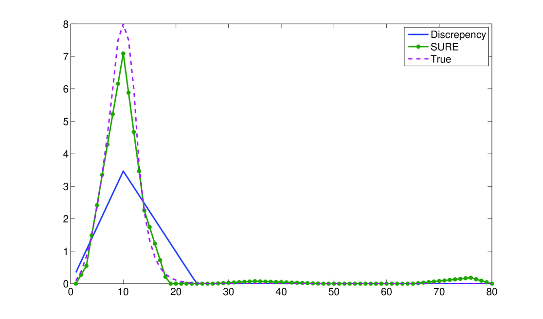
To evaluate the gradient of the estimate, we used the Monte-Carlo SURE approach proposed in [39]. Evidently, the SURE method leads to superior performance. The MSE using the SURE approach in this example is 0.10 while the discrepancy strategy leads to an MSE of 1.16.

VII Regularized SURE Method

A crucial element in guaranteeing success of the SURE method is to choose a good parameterization of ${{\bf h}}({\mathbf{u}})$. However, in many contexts, such a structure may be hard to find. On the other hand, letting the SURE criterion select many free parameters can deteriorate its performance. One way to treat this inherent tradeoff is by regularization. Thus, instead of minimizing the SURE objective we suggest minimizing a regularized version:

$$S({{\bf h}},\lambda)=S({{\bf h}})+\lambda r({{\bf h}}({\mathbf{u}}))$$ (63)

where $\lambda$ is a regularization parameter and $r({{\bf h}}({\mathbf{u}}))$ is a regularization function. For example, we may choose $r({\mathbf{v}})=\|{\mathbf{v}}\|$ where the norm is arbitrary. The parameter $\lambda$ is determined by applying the conventional SURE (29) (or (38)) to the estimate ${{\bf h}}({\mathbf{u}},\lambda)$ resulting from solving (63) with $\lambda$ fixed.

As an example, consider the iid Gaussian model in which ${{{\bf x}}}=\mbox{\boldmath{$\theta$}}+{\bf w}$ where ${\bf w}$ is a Gaussian noise vector with iid zero-mean components of variance $\sigma^{2}$. Assuming that $\theta$ represents the wavelet coefficients of some underlying signal ${{{\bf x}}}$, a popular estimation strategy is wavelet denoising in which each component of ${{{\bf x}}}$ is replaced by a soft or hard-thresholded version. In particular, in their landmark paper, Donoho and Johnstone [11] developed a soft-threshold wavelet denoising method in which

$$\hat{\theta}_{i}=\left\{\begin{array}[]{ll}|x_{i}|-t,&|x_{i}|\geq t;\\ 0,&|x_{i}|<t,\end{array}\right.$$ (64)

where $t$ is a threshold value. They suggest selecting $t$ to minimize the SURE criterion, and refer to the resulting estimate as SureShrink (to be more precise, in SureShrink $t$ is determined by SURE only if it lower than some upper limit). In developing the SureShrink method, the function ${{\bf h}}({{{\bf x}}})$ is restricted to be a component-wise soft threshold. The motivation for this choice is that the wavelet coefficients below a certain level tend to be sparse. It is well known that soft-thresholding can be obtained as the solution to a LS criterion with an $\ell_{1}$ penalty:

$$\min\left\{\|{{{\bf x}}}-\mbox{\boldmath{$\theta$}}\|^{2}+\lambda\|\mbox{\boldmath{$\theta$}}\|_{1}\right\}.$$ (65)

Thus, in principle we can view the SureShrink approach as a 2-step procedure: We first determine the estimate that minimizes an $\ell_{1}$ penalized LS criterion. We then choose the penalization factor to minimize SURE.

Instead, we suggest choosing an estimate that directly minimizes an $\ell_{1}$ regularized SURE objective, where the only assumption we make is that the processing is performed component wise. Thus, $\hat{\theta}_{i}=\alpha_{i}x_{i}$ for some coefficients $\alpha_{i}({{{\bf x}}})\geq 0$. Since ${\mathbf{u}}=(1/\sigma^{2})x_{i}$, $h_{i}({\mathbf{u}})=\sigma^{2}\alpha_{i}u_{i}$. With this choice of ${{\bf h}}({\mathbf{u}})$, minimizing (63) is equivalent to minimizing the following objective:

$$S(\mbox{\boldmath{$\alpha$}},\lambda)=\sum_{i=1}^{n}\alpha_{i}^{2}x_{i}^{2}+2\sum_{i=1}^{n}\alpha_{i}\left(\sigma^{2}-x_{i}^{2}\right)+\lambda\sum_{i=1}^{n}|\alpha_{i}||x_{i}|.$$ (66)

The optimal choice of $\alpha_{i}\geq 0$ is

$$\alpha_{i}=\left[1-\frac{\sigma^{2}+\lambda|x_{i}|}{x_{i}^{2}}\right]_{+}.$$ (67)

The resulting estimate can be viewed as a soft-thresholding method, with a particular choice of shrinkage (different than the standard approach (64)) when the value of $x_{i}$ exceeds the threshold. The precise threshold value is equal to the largest value $x_{i}$ for which $\alpha_{i}=0$ and is given by

$$t=\frac{1}{2}\left(\lambda+\sqrt{\lambda^{2}+4\sigma^{2}}\right).$$ (68)

To choose $\lambda$, we substitute the estimate $\hat{\theta}_{i}=\alpha_{i}(\lambda)x_{i}$ with $\alpha_{i}(\lambda)$ given by (67) into the SURE criterion (48) with ${{\bf P}}={{\bf I}}$, and minimize with respect to $\lambda$. The value of $\lambda$ can be easily determined numerically.

To demonstrate the advantage of our method over conventional soft-thresholding we implemented our approach on the examples taken from [11]. Specifically, we used the test functions Blocks, Bumps, HeaviSine and Doppler defined in [11]. The length of all signals is $2048$ and the noise variance is $\sigma^{2}=4$. We used the Daubechies 8 symmetrical wavelet, and $L=5$ levels are considered. In Table III we report the empirical MSE values of the original noisy signals, and 3 wavelet denoising schemes: SureShrink which is the method of [11] with the threshold selected using SURE, our proposed regularized SURE method (RSURE), and OracleShrink which is a soft-threshold where the threshold value is selected to minimize the squared-error between the true unknown wavelet coefficient, and its denoised version. Clearly this approach is only for comparison and serves as a benchmark on the best possible performance that can be obtained using any soft threshold.

TABLE III: MSE for Different Soft Denoising Schemes

	Blocks	Bumps	HeaviSine	Doppler
Original	4.054	4.072	4.153	3.945
SureShrink	0.744	0.875	0.205	0.290
RSure	0.694	0.816	0.169	0.273
OracleShrink	0.690	0.828	0.118	0.283

As can be seen from the table, the regularized SURE method performs better in all cases than SureShrink. It is also interesting to see that it sometimes even outperforms OracleShrink which is based on the true unknown $\theta$. The reason the performance can be better than the oracle is that the shrinkage performed in RSURE is different than the conventional soft threshold.

In Table IV we repeat our experiments where now we use the estimates resulting from the standard SURE criterion. Specifically, we consider the positive-part Stein estimate (51) referred to as SteinShrink and the estimate (57) which we refer to as ScalarShrink.

TABLE IV: MSE for Different Denoising Schemes

	Blocks	Bumps	HeaviSine	Doppler
ScalarShrink	1.043	1.362	0.161	0.594
SteinShrink	1.681	1.730	1.508	1.413

Evidently, using the SURE estimate without regularization deteriorates the performance significantly. Thus, SURE alone is not generally sufficient to obtain good estimates. However, adding regularization dramatically improves the behavior without the need to pre-specify the desired structure.

Finally, in Table V we repeat the experiments of Table III to determine the threshold values, but once the values are found we apply hard-thresholding on the coefficients.

TABLE V: MSE for Different Hard-Thresholding Schemes

	Blocks	Bumps	HeaviSine	Doppler
SureShrink	1.902	1.961	0.988	0.630
RSure	1.560	1.912	0.766	0.700

As can be seen from the table, even though the thresholding operation is now the same in both methods, RSURE performs significantly better. Thus, the threshold determined from this method is superior to that resulting from the SURE criterion without regularization. Here again the importance of regularization is demonstrated.

VIII Conclusion

In this paper, we developed an unbiased estimate of the MSE in multivariate exponential families by extending the SURE method. This generalized principle can now be used in exponential multivariate estimation problems to develop estimators with improved performance over existing approaches. As an application, we suggested a new strategy for choosing the regularization parameter in penalized inverse problems. We demonstrated via several examples that this method can significantly improve the MSE over the standard GCV and discrepancy approaches. We also suggested a regularized SURE criterion for selecting estimators without the need for pre-specifying their structure. Applying this objective in the context of wavelet denoising, we proposed a new type of soft-thresholding which minimizes a penalized estimate of the MSE. As we demonstrated, this strategy can lead to improved MSE behavior in comparison with soft and hard thresholding methods.

The main contribution of this work is in introducing the generalized SURE criterion and the regularized SURE method and demonstrating their applicability in several examples. In future work, we intend to develop these applications in more detail and further explore the practical use of the proposed design objectives.

IX Acknowledgement

The author would like to thank Zvika Ben-Haim and Michael Elad for many fruitful discussions.

Yonina C. Eldar (S’98–M’02–SM’07) Yonina C. Eldar received the B.Sc. degree in Physics in 1995 and the B.Sc. degree in Electrical Engineering in 1996 both from Tel-Aviv University (TAU), Tel-Aviv, Israel, and the Ph.D. degree in Electrical Engineering and Computer Science in 2001 from the Massachusetts Institute of Technology (MIT), Cambridge.

From January 2002 to July 2002 she was a Postdoctoral Fellow at the Digital Signal Processing Group at MIT. She is currently an Associate Professor in the Department of Electrical Engineering at the Technion - Israel Institute of Technology, Haifa, Israel. She is also a Research Affiliate with the Research Laboratory of Electronics at MIT. Her research interests are in the general areas of signal processing, statistical signal processing, and computational biology.

Dr. Eldar was in the program for outstanding students at TAU from 1992 to 1996. In 1998, she held the Rosenblith Fellowship for study in Electrical Engineering at MIT, and in 2000, she held an IBM Research Fellowship. From 2002-2005 she was a Horev Fellow of the Leaders in Science and Technology program at the Technion and an Alon Fellow. In 2004, she was awarded the Wolf Foundation Krill Prize for Excellence in Scientific Research, in 2005 the Andre and Bella Meyer Lectureship, in 2007 the Henry Taub Prize for Excellence in Research, and in 2008 the Hershel Rich Innovation Award and Award for Women with Distinguished Contributions. She is a member of the IEEE Signal Processing Theory and Methods technical committee, an Associate Editor for the IEEE Transactions on Signal Processing, the EURASIP Journal of Signal Processing, and the SIAM Journal on Matrix Analysis and Applications, and on the Editorial Board of Foundations and Trends in Signal Processing.

References

- [1] C. Stein, “Inadmissibility of the usual estimator for the mean of a multivariate normal distribution,” in Proc. Third Berkeley Symp. Math. Statist. Prob. 1956, vol. 1, pp. 197–206, University of California Press, Berkeley.
- [2] W. James and C. Stein, “Estimation of quadratic loss,” in Proc. Fourth Berkeley Symp. Math. Statist. Prob. 1961, vol. 1, pp. 361–379, University of California Press, Berkeley.
- [3] W. E. Strawderman, “Proper Bayes minimax estimators of multivariate normal mean,” Ann. Math. Statist., vol. 42, pp. 385–388, 1971.
- [4] K. Alam, “A family of admissible minimax estimators of the mean of a multivariate normal distribution,” Ann. Statist., vol. 1, pp. 517–525, 1973.
- [5] J. O. Berger, “Admissible minimax estimation of a multivariate normal mean with arbitrary quadratic loss,” Ann. Statist., vol. 4, no. 1, pp. 223– 226, Jan. 1976.
- [6] Z. Ben-Haim and Y. C. Eldar, “Blind minimax estimators: Improving on least squares estimation,” in IEEE Workshop on Statistical signal Processing (SSP’05), Bordeaux, France, July 2005.
- [7] Z. Ben-Haim and Y. C. Eldar, “Blind minimax estimation,” IEEE Trans. Inform. Theory, vol. 53, pp. 3145–3157, Sep. 2007.
- [8] Y. C. Eldar, A. Ben-Tal, and A. Nemirovski, “Robust mean-squared error estimation in the presence of model uncertainties,” IEEE Trans. Signal Processing, vol. 53, pp. 168–181, Jan. 2005.
- [9] C. M. Stein, “Estimation of the mean of a multivariate distribution,” Proc. Prague Symp. Asymptotic Statist., pp. 345–381, 1973.
- [10] C. M. Stein, “Estimation of the mean of a multivariate normal distribution,” Ann. Stat., vol. 9, no. 6, pp. 1135–1151, Nov. 1981.
- [11] D. L. Donoho and I. M. Johnstone, “Adapting to unknown smoothness via wavelet shrinkage,” J. Am. Stat. Assoc., vol. 90, no. 432, pp. 1200–1224, Dec. 1995.
- [12] X. P. Zhang and M. D. Desai, “Adapting denoising based on SURE risk,” IEEE Signal Process. Lett., vol. 5, no. 10, pp. 265–267, 1998.
- [13] F. Luisier, T. Blu, and M. Unser, “A new SURE approach to image denoising: Interscale orthonormal wavelet thresholding,” IEEE Trans. Image Process., vol. 16, no. 3, pp. 593–606, 2007.
- [14] A. Benazza-Benyahia and J.-C. Pesquet, “Building robust wavelet estimators for multicomponent images using Stein’s principle,” IEEE Trans. Image Process., vol. 14, no. 11, pp. 1814–1830, 2005.
- [15] R. Averkamp and C. Houdre, “Stein estimation for infinitely divisible laws,” ESAIM: Probability and Statistics, p. 269, 2006.
- [16] H. M. Hudson, “A natural identity for exponential families with applications in multiparameter estimation,” Ann. Statist., vol. 6, no. 3, pp. 473–484, 1978.
- [17] J. Berger, “Improving on inadmissible estimators in continuous exponential families with applications to simultaneous estimation of gamma scale parameters,” Ann. Stat., vol. 8, no. 3, pp. 545–571, 1980.
- [18] J. T. Hwang, “Improving upon standard estimators in discrete exponential families with applications to Poisson and negative binomial cases,” Ann. Statist., vol. 10, no. 3, pp. 857–867, 1982.
- [19] E. Pitman, “Sufficient statistics and intrinsic accuracy,” Proc. Camb. phil. Soc., vol. 32, pp. 567–579, 1936.
- [20] G. Darmois, “Sur les lois de probabilites a estimation exhaustive,” C.R. Acad. sci. Paris, vol. 200, pp. 1265–1266, 1935.
- [21] B. Koopman, “On distribution admitting a sufficient statistic,” Trans. Amer. math. Soc., vol. 39, pp. 399–409, 1936.
- [22] E. L. Lehmann and G. Casella, Theory of Point Estimation, New York, NY: Springer-Verlag, Inc., second edition, 1998.
- [23] A. N. Tikhonov and V. Y. Arsenin, Solution of Ill-Posed Problems, Washington, DC: V.H. Winston, 1977.
- [24] J. Rice, “Choice of smoothing parameter in deconvolution problems,” Contemporary Math., vol. 59, pp. 137–151, 1986.
- [25] L. Desbat and D. Girard, “The “minimum reconstruction error” choice of regularization parameters: Some effective methods and their application to deconvolution problem,” SIAM J. Sci. Comput., vol. 16, no. 6, pp. 1387–1403, Nov. 1995.
- [26] N. P. Galatsanos and A. K. Katsaggelos, “Methods for choosing the regularization parameter and estimating the noise variance in image restoration and their relation,” IEEE Trans. Image Process., vol. 1, no. 3, pp. 322–336, 1992.
- [27] P. C. Hansen, “The use of the L-curve in the regularization of discrete ill-posed problems,” SIAM J. Sci. Stat. Comput., vol. 14, pp. 1487–1503, 1993.
- [28] M. Hanke and P. C. Hansen, “Regularization methods for large-scale problems,” Surveys Math. Indust., vol. 3, no. 4, pp. 253–315, 1993.
- [29] A. Björck, Numerical Methods for Least-Squares Problems, Philadelphia, PA: SIAM, 1996.
- [30] R. Molina, A. K. Katsaggelos, and J. Mateos, “Bayesian and regularization methods for hyperparameter estimation in image restoration,” IEEE Trans. Image Process., vol. 8, no. 2, pp. 231–246, 1999.
- [31] W. C. Karl, “Regularization in image restoration and reconstruction,” in Handbook of Image and Video Processing, A. Bovik, Ed., pp. 183 –202. ELSEVIER, 2nd edition, 2005.
- [32] G.H. Golub, M. Heath, and G. Wahba, “Generalized cross-validation as a method for choosing a good ridge parameter,” Technometrics, vol. 21, no. 2, pp. 215–223, May 1979.
- [33] S. M. Kay, Fundamentals of Statistical Signal Processing: Estimation Theory, Upper Saddle River, NJ: Prentice Hall, Inc., 1993.
- [34] E. H. Lieb and M. Loss, Analysis, American Mathematical Society, second edition, 2001.
- [35] A. J. Baranchik, “Multiple regression and estimation of the mean of a multivariate normal distribution,” Tech. Rep. 51, Stanford University, 1964.
- [36] P. C. Hansen, J. G. Nagy, and D. P. OLeary, Deblurring Images: Matrices, Spectra, and Filtering, Philadelphia, PA: SIAM, 2006.
- [37] M. Grant and S. Boyd, “CVX: Matlab software for disciplined convex programming (web page and software),” March 2008, http://stanford.edu/~boyd/cvx.
- [38] P. C. Hansen, “Regularization tools, a matlab package for analysis of discrete regularization problems,” Numerical Algorithms, vol. 6, pp. 1–35, 1994.
- [39] S. Ramani, T. Blu, and M. Unser, “Blind optimization of algorithm parameters for signal denoising by Monte-Carlo SURE,” in Proc. Int. Conf. Acoust., Speech, Signal Processing (ICASSP-2008), (Las-Vegas, NV), April 2008.