Flow instabilities of magnetic flux tubes

Abstract

Context. The stability properties of toroidal magnetic flux tubes are relevant for the storage and emergence of magnetic fields in the convective envelope of cool stars. In addition to buoyancy- and magnetic tension-driven instabilities, flux tubes are also susceptible to an instability induced by the hydrodynamic drag force.

Aims. Following our investigation of the basic instability mechanism in the case of straight flux tubes, we now investigate the stability properties of magnetic flux rings. The focus lies on the influence of the specific shape and equilibrium condition on the thresholds of the friction-induced instability and on their relevance for emerging magnetic flux in solar-like stars.

Methods. We substitute the hydrodynamic drag force with Stokes law of friction to investigate the linear stability properties of toroidal flux tubes in mechanical equilibrium. Analytical instability criteria are derived for axial symmetric perturbations and for flux rings in the equatorial plane by analysing the sequence of principal minors of the coefficient matrices of dispersion polynomials. The general case of non-equatorial flux rings is investigated numerically by considering flux tubes in the solar overshoot region.

Results. The friction-induced instability occurs when an eigenmode reverses its direction of propagation due to advection, typically from the retrograde to the prograde direction. This reversal requires a certain relative velocity difference between plasma inside the flux tube and the environment. Since for flux tubes in mechanical equilibrium the relative velocity difference is determined by the equilibrium condition, the instability criterion depends on the location and field strength of the flux ring. The friction-induced instability sets in at lower field strengths than buoyancy- and tension-driven instabilities. Its threshold is independent of the strength of friction, but the growth rates depend on the strength of the frictional coupling between flux tube and environment.

Conclusions. The friction-induced instability lowers the critical magnetic field strength beyond which flux tubes are subject to growing perturbations. Since its threshold does not depend explicitely on the friction parameter, this mechanism also applies in case of the quadratic velocity dependence of the hydrodynamic drag force. Whereas buoyancy- and tension-driven instabilities depend on the magnetic field strength alone, the dependence of hydrodynamic drag on the tube diameter gives rise to an additional dependence of growth times on the magnetic flux.

1 Introduction

The magnetic field observed on the surfaces of cool, solar-like stars is assumed to originate in the bottom of the stellar convection zone. It is amplified by the shear flow in the tachocline and stored in the stably stratified overshoot region at the interface to the radiative core. The toroidal magnetic fields are subject to perturbations through overshooting gas plumes penetrating from the convection zone above. Beyond a critical field strength, unstable perturbations lead to growing magnetic flux loops, which rise through the convection zone and eventually emerge at the stellar surface (e.g. 1982A&A...106...58S; 1996A&A...314..503S). In the solar overshoot region, critical field strengths are of the order of $10^{5}{\,{\rm G}}$ (e.g. 1993GAFD...72..209; 1995GAFD...81..233). Simulations of rising flux tubes with such initial field strengths yield emergence properties which are consistent with observed properties of sunspots such as their eruption latitudes, tilt angles, proper motions, and asymmetries between the leading and the following component of bipolar spot groups (1993A&A...272..621D; 1994ApJ...436..907F; 1994SoPh..153..449M; 1995ApJ...441..886C).

The stability properties of magnetic flux tubes are relevant for the amplification, storage, and emergence of magnetic fields. An efficient generation of magnetic flux requires the field to remain within the convection zone for time periods which are comparable with or longer than the amplification timescale of the (here, unspecified) dynamo mechanism. Instability mechanisms limit the storage time and lead to their leakage of magnetic fields from the overshoot region with field-dependent growth times. The main driving mechanism of unstable, non-axisymmetric perturbations is magnetic buoyancy, which gives rise to undulatory, Parker-type instabilities (1955ApJ...121..491P). If the flux tube dynamics is dominated by the magnetic tension force, an axial-symmetric poleward slip instability can occur (1982A&A...106...58S).

The hydrodynamic drag force reduces the relative motion of a flux tube perpendicular to its environment, similar to the case of a solid cylinder immersed in an external flow. The intrinsically dissipative interaction with the environment can cause under certain conditions the onset of flux tube instabilities (e.g. 1988JETP...67.1594R; 1997SoPh..176..285J). A friction-induced instability occurs if the relative flow velocity along the magnetic flux tube is higher than a critical value. In paper II of this series (2007A&A...469...11H), we have investigated friction-induced instabilities of straight, horizontal flux tubes with parallel flows to elucidate the basic instability mechanism. In that case, the velocity difference between the internal and external plasma was a free parameter. Here we consider magnetic flux rings in a stratified environment to investigate the influence of the toroidal geometry and of the equilibrium condition on the stability properties. Both aspects affect the velocity difference between the internal and external plasma.

In Sect. 2 we describe the linearisation of the equations of motion in the framework of the thin flux tube-model, including a frictional interaction with the environment. In the linear stability analysis in Sect. 3, analytical instability criteria are derived for some special cases. The general case is analysed numerically on the basis of flux rings located in the solar overshoot region. Section 4 contains the discussion of the results and Sect. 5 the conclusions.

2 Model description

2.1 Thin flux tube approximation

The stability analysis is carried out in the framework of the thin flux tube approximation (1981A&A...102..129S). The radius of the flux tube is small compared with the radius of curvature, the wavelength of a perturbation, and the pressure scale height. Cross-sectional variations are taken to be negligible. All quantities are given by their values on the tube axis and are functions of time, $t$, and arc length, $s$, only. The flux tube is assumed to always retain a circular cross section.

The dynamics of the magnetic flux tube is determined through the equation of motion

$$\rho\frac{d}{dt}\@vec{u}=-\nabla\left(p+\frac{\@vec{B}^{2}}{8\pi}\right)+\rho\@vec{g}+\@vec{n}\frac{\@vec{B}^{2}}{4\pi}\,\kappa+\@vec{t}\frac{\partial}{\partial s}\frac{\@vec{B}^{2}}{8\pi}+2\rho\left(\@vec{u}\times\@vec{\Omega}\right)+\@vec{f}_{\scriptstyle\mathrm{D}}\ ,$$ (1)

where $\@vec{u}$ is the plasma velocity, $\@vec{B}$ is the magnetic field, $\rho$ is the density, $p$ is the gas pressure, $\kappa$ is the curvature of the tube, and $\@vec{\Omega}$ is the constant rotation vector of the star. For most but the fastest rotating stars the contribution of the centrifugal acceleration to the effective gravitation is small. We therefore take $\@vec{g}\simeq-g\@vec{e}_{r}$, with $\@vec{e}_{r}$ being the radial unit vector in a spherical coordinate system and $g\,(=\textrm{const})$ being the local gravitation. The adopted coordinate system is the tripod co-moving with the magnetic flux tube (Frenet basis), consisting of the tangential vector $\@vec{t}$, the normal vector $\@vec{n}$, and the binormal vector $\@vec{b}$. The tangential vector defines the axis of the flux tube, implying $\@vec{B}=B\@vec{t}$.

2.2 Drag force

In the limit of infinite conductivity, plasma cannot cross the magnetic surface of a flux tube. Consequently, a motion of the flux tube perpendicular to its tube axis implies a flow of the external plasma around the tube. Analogous to a cylinder immersed in a non-ideal streaming fluid, this flow gives rise to a hydrodynamic drag force

$$\@vec{f}_{\scriptstyle\mathrm{D}}=-\rho_{\scriptstyle\mathrm{e}}\frac{C_{\scriptstyle\mathrm{D}}}{\pi a}\left|\@vec{u}_{\scriptstyle\mathrm{rel,\perp}}\right|\@vec{u}_{\scriptstyle\mathrm{rel,\perp}}\ ,$$ (2)

where $\rho_{\scriptstyle\mathrm{e}}$ is the density of the external plasma, $a$ is the tube radius, $C_{\scriptstyle\mathrm{D}}$ is the (empirical) drag coefficient, and $\@vec{u}_{\scriptstyle\mathrm{rel,\perp}}$ is the component perpendicular to the tube axis of the velocity difference between the internal and the external plasma. In the reference frame co-rotating with the star, the external plasma is at rest and the relative perpendicular flow velocity thus given by

$$\@vec{u}_{\scriptstyle\mathrm{rel,\perp}}=\@vec{u}-\left(\@vec{u}\cdot\@vec{t}\right)\@vec{t}\ .$$ (3)

In stationary equilibrium, the plasma flow inside the flux tube is parallel to the tube axis. Owing to its quadratic dependence on the velocity, the hydrodynamic drag force drops out of the linearised equation of motion (e.g. 1993GAFD...72..209). To investigate the principal influence of friction on the stability properties of magnetic flux tubes, we consider the case of a linear velocity dependence according to Stokes’s law:

$$\@vec{f}_{\scriptstyle\mathrm{D}}\rightarrow\@vec{f}_{\scriptstyle\mathrm{St}}=-\rho_{\scriptstyle\mathrm{e}}\alpha\@vec{u}_{\scriptstyle\mathrm{rel,\perp}}\ .$$ (4)

The friction parameter, $\alpha>0$, is taken to be constant.

2.2.1 External stratification

Disregarding any differential rotation or meridional circulation, the stellar stratification in the co-rotating reference frame is determined through

$$\nabla p_{\scriptstyle\mathrm{e}}=\rho_{\scriptstyle\mathrm{e}}\,\@vec{g}\ ,$$ (5)

where $p_{\scriptstyle\mathrm{e}}$ and $\rho_{\scriptstyle\mathrm{e}}$ are the external gas pressure and density, respectively. The flux tube is in lateral pressure balance with its field-free environment:

$$p_{\scriptstyle\mathrm{e}}=p+\frac{B^{2}}{8\pi}\ .$$ (6)

Subtracting Eq. (5) from Eq. (1) yields

$$\frac{d}{dt}\@vec{u} = \frac{\Delta\rho}{\rho}\@vec{g}_{\scriptstyle\mathrm{eff}}+\@vec{n}\kappa\frac{B^{2}}{4\pi\rho}+\@vec{t}\frac{1}{\rho}\frac{\partial}{\partial s}\frac{B^{2}}{8\pi}+2\left(\@vec{u}\times\@vec{\Omega}\right)-\frac{\rho_{\scriptstyle\mathrm{e}}}{\rho}\alpha\@vec{u}_{\scriptstyle\mathrm{\perp}}\ ,$$ (7)

where $\Delta\rho=\rho-\rho_{\scriptstyle\mathrm{e}}$ is the density contrast. Equation (7) is the starting point for the linear stability analysis.

2.3 Linearised equation of motion

2.3.1 Equilibrium condition

We consider magnetic flux rings in mechanical equilibrium located parallel to the equatorial plane. A detailed description of this equilibrium and how it is obtained is given by 1992A&A...264..686M and 1995ApJ...441..886C.

In the following, the index ‘0’ indicates equilibrium values. Since the equilibrium flux ring is axially symmetric, the tangential component of Eq. (7) vanishes. From the binormal component follows that the density contrast is nil, because buoyancy provides the only force component parallel to the rotation axis. With $\Delta\rho_{\scriptstyle\mathrm{0}}=0$ the normal component of Eq. (7) yields

$$u_{0}^{2}+2u_{0}v_{\scriptstyle\mathrm{e,0}}-c_{\scriptstyle\mathrm{A,0}}^{2}=0\ ,$$ (8)

where $c_{\scriptstyle\mathrm{A,0}}=B_{0}/\sqrt{4\pi\rho_{0}}$ is the Alfvén velocity and $v_{\scriptstyle\mathrm{e,0}}=\Omega/\kappa_{\scriptstyle\mathrm{0}}$ is the rotation velocity of the tube’s environment. Equation (8) determines the velocity,

$$u_{0}=v_{\scriptstyle\mathrm{e,0}}\left(\sqrt{1+\left(\frac{c_{\scriptstyle\mathrm{A,0}}}{v_{\scriptstyle\mathrm{e,0}}}\right)^{2}}-1\right)>v_{\scriptstyle\mathrm{e,0}}\ ,$$ (9)

of the plasma inside the flux ring which is required to balance the magnetic tension force through Coriolis and inertial forces. This internal plasma flow is in prograde direction. We shall refer to the dimensionless quantity

$$\eta=\frac{c_{\scriptstyle\mathrm{A,0}}}{v_{\scriptstyle\mathrm{e,0}}}=\frac{c_{\scriptstyle\mathrm{A,0}}\,\kappa_{0}}{\Omega}=\frac{c_{\scriptstyle\mathrm{A,0}}}{\Omega\,R_{0}}=\frac{c_{\scriptstyle\mathrm{A,0}}}{\Omega\,r_{0}\,\cos\lambda_{0}}$$ (10)

as the equilibrium parameter of the flux tube, where $R_{0}$ is the equilibrium radius of the flux ring in cylindrical coordinates, and $r_{0}$ and $\lambda_{0}$ its radius and latitude, respectively, in spherical coordinates.

2.3.2 First-order perturbations

The linear stability properties are determined through the first-order perturbation terms of Eq. (7). In the co-moving Frenet basis, the tangential, normal, and binormal components are

$$\left(\frac{d}{dt}\@vec{u}\right)_{1}\cdot\@vec{t}_{0}-\left(\frac{1}{\rho}\frac{\partial}{\partial s}\frac{B^{2}}{8\pi}\right)_{1}+\kappa_{0}c_{\scriptstyle\mathrm{A,0}}^{2}\left(\@vec{n}_{0}\cdot\@vec{t}_{1}\right)-2\Omega\left(\@vec{n}_{0}\cdot\@vec{u}_{1}\right) = 0$$ (11)

$$\left(\frac{d}{dt}\@vec{u}\right)_{1}\cdot\@vec{n}_{0}-\frac{\Delta\rho}{\rho}\bigg{|}_{1}g_{0}g_{n}+2\Omega\left(\@vec{t}_{0}\cdot\@vec{u}_{1}\right)+\alpha\left(\@vec{u}_{\scriptstyle\mathrm{rel,\perp,1}}\cdot\@vec{n}_{0}\right)$$

$${}-\kappa_{0}c_{\scriptstyle\mathrm{A,0}}^{2}\left(\frac{\kappa_{1}}{\kappa_{0}}+2\frac{B_{1}}{B_{0}}-\frac{\rho_{1}}{\rho_{0}}\right) = 0$$ (12)

$$\left(\frac{d}{dt}\@vec{u}\right)_{1}\cdot\@vec{b}_{0}-\frac{\Delta\rho}{\rho}\bigg{|}_{1}g_{0}g_{b}+\kappa_{0}c_{\scriptstyle\mathrm{A,0}}^{2}\left(\@vec{n}_{0}\cdot\@vec{b}_{1}\right)+\alpha\left(\@vec{u}_{\scriptstyle\mathrm{rel,\perp,1}}\cdot\@vec{b}_{0}\right) = 0\ ,$$ (13)

with $g_{n}=\left(\@vec{g}\cdot\@vec{n}_{0}\right)/g_{0}$ and $g_{b}=\left(\@vec{g}\cdot\@vec{b}_{0}\right)/g_{0}$. For magnetic flux rings perpendicular to the stellar rotation axis it is $\@vec{t}_{0}=\@vec{e}_{\phi},\@vec{n}_{0}=-\@vec{e}_{R}$, and $\@vec{b}_{0}=\@vec{e}_{z}$. The first-order perturbations of all quantities (indicated by the index ‘1’) depend linearly on the Lagrangian displacement vector $\@vec{\xi}=\left(\xi_{t},\xi_{n},\xi_{b}\right)^{T}$, and are summarised in Appendix A. Their detailed derivation can be found, for example, in 1993GAFD...72..209; 1995GAFD...81..233 and 1998GApFD..89...75S.

Except for the drag force, which comes from the perturbation of the exterior, the velocity of the external plasma is taken to be unchanged by the perturbation of the flux tube, that is, $\@vec{u}_{\scriptstyle\mathrm{e,1}}=0$. The perturbations of the internal flow velocity and of the tube’s axis given by Eqs. (101) and (97), respectively, yield the perturbation of the relative perpendicular flow velocity:

$$\@vec{u}_{\scriptstyle\mathrm{rel,\perp,1}}=\@vec{u}_{1}-\left(\@vec{u}_{1}\cdot\@vec{t}_{0}\right)\@vec{t}_{0}-u_{0}\@vec{t}_{1}=\xi_{n,t}\@vec{n}_{0}+\xi_{b,t}\@vec{b}_{0}\ .$$ (14)

Derivatives with respect to time and arc length are indicated by the indices $t$ and $s$, respectively. At the bottom of stellar convection zones, the plasma pressure is typically much higher than the magnetic pressure. The stability analysis is therefore carried out in the approximation $\beta=8\pi p_{0}/B_{0}^{2}\gg 1$. In the limit of an infinite radius of curvature and vanishing stellar rotation (i.e. $\kappa\rightarrow 0,\Omega\rightarrow 0$), Eqs. (11)-(13) reduce to the case of a horizontal flux tube in a stratified atmosphere, which was investigated in 2007A&A...469...11H. Note that the present investigation disregards the possible influence of enhanced inertia (factor $\mu$ in 2007A&A...469...11H), owing to its conceptual difficulties in the case of curved thin flux tubes (cf. 1996A&A...312..317M, and references therein).

2.3.3 Non-dimensional form

The linearised equations of motion are transferred to non-dimensional form by multiplying Eqs. (11)-(13) with the timescale $\tau=1/\Omega$, which yields

$$\tau^{2}\@vec{\xi}_{,tt}+\mathcal{M}_{st}\frac{\tau}{\kappa_{0}}\@vec{\xi}_{,st}+\mathcal{M}_{ss}\frac{1}{\kappa_{0}^{2}}\@vec{\xi}_{,ss}+\mathcal{M}_{t}\tau\@vec{\xi}_{,t}+\mathcal{M}_{s}\frac{1}{\kappa_{0}}\@vec{\xi}_{,s}+\mathcal{M}_{\xi}\@vec{\xi}=\@vec{0}\ .$$ (15)

The coefficient matrices are

$$\mathcal{M}_{st} = 2\,Ro\,\mathcal{E}$$ (16)

$$\mathcal{M}_{ss} = -2\,Ro\,\mathcal{E}$$ (17)

$$\mathcal{M}_{t} = 2\,\left(Ro+1\right)\,\mathcal{Y}+\tilde{\alpha}\,\mathcal{X}$$ (18)

$$\mathcal{M}_{s} = -2\,Ro\,\mathcal{Y}+\frac{\eta^{2}}{\gamma f_{0}}\left(g_{\scriptstyle\mathrm{n}}\,\mathcal{Y}+g_{\scriptstyle\mathrm{b}}\,\mathcal{Z}\right)$$ (19)

$$\mathcal{M}_{\xi} = \tilde{\omega}_{\scriptstyle\mathrm{MBV}}^{2}\left(\begin{array}[]{ccc}0&0&0\\ 0&g_{\scriptstyle\mathrm{n}}g_{\scriptstyle\mathrm{n}}&g_{\scriptstyle\mathrm{n}}g_{\scriptstyle\mathrm{b}}\\ 0&g_{\scriptstyle\mathrm{n}}g_{\scriptstyle\mathrm{b}}&g_{\scriptstyle\mathrm{b}}g_{\scriptstyle\mathrm{b}}\end{array}\right)-\frac{\eta^{2}}{\gamma f_{0}}\left(\begin{array}[]{ccc}0&0&0\\ 0&2g_{\scriptstyle\mathrm{n}}&g_{\scriptstyle\mathrm{b}}\\ 0&g_{\scriptstyle\mathrm{b}}&0\end{array}\right)\ ,$$ (26)

where

$$\mathcal{X}=\left(\begin{array}[]{ccc}0&0&0\\ 0&1&0\\ 0&0&1\end{array}\right),\quad\mathcal{Y}=\left(\begin{array}[]{ccc}0&-1&0\\ 1&0&0\\ 0&0&0\end{array}\right),\quad\mathcal{Z}=\left(\begin{array}[]{ccc}0&0&-1\\ 0&0&0\\ 1&0&0\end{array}\right)\ ,$$ (36)

$\mathcal{E}$ is the unity matrix,

$$Ro=\frac{u_{0}\kappa_{0}}{\Omega}=\sqrt{1+\eta^{2}}-1$$ (37)

is the Rossby number,

$$f_{0}=H_{p}\,\kappa_{0}$$ (38)

is the ratio between the local pressure scale height and the radius of curvature, and $\tilde{\alpha}=\tau\alpha$ is the dimensionless friction parameter. The (dimensionless) magnetic Brunt-Väisälä frequency,

$$\tilde{\omega}_{\scriptstyle\mathrm{MBV}}^{2} = \tau^{2}\omega_{\scriptstyle\mathrm{MBV}}^{2}=-\frac{\eta^{2}}{2f_{0}^{2}}\left[\beta\,\delta-\frac{2}{\gamma}\,\left(\frac{1}{\gamma}-\frac{1}{2}\right)\right]$$ (39)

$$= \tau^{2}\,N^{2}+\frac{\eta^{2}}{\gamma^{2}f_{0}^{2}}\left(1-\frac{\gamma}{2}\right)\ ,$$

is a measure for axisymmetric buoyancy oscillations of magnetic flux rings. Owing to the stabilising effect of the magnetic field, its value is higher than the non-magnetic Brunt-Väisälä frequency,

$$N^{2}=-\frac{g}{H_{\scriptstyle\mathrm{p}}}\delta\ ,$$ (40)

which depends on the superadiabaticity $\delta=\nabla-\nabla_{\scriptstyle\mathrm{ad}}$ and quantifies the stability of the stratification against convective turnover. Positive (negative) values of $\omega_{\scriptstyle\mathrm{MBV}}^{2}$ and $N^{2}$ indicate stable (unstable) perturbations of the plasma in the presence and absence of a magnetic field, respectively.

2.3.4 Solar reference case

For the numerical evaluation of linear stability properties, we shall refer to a magnetic flux ring located in the middle of the solar overshoot region. At radius $r_{0}=5.07\cdot 10^{10}{\,{\rm cm}}$, the local density is $\rho_{0}=0.15{\,{\rm g/cm^{3}}}$, the gravitation is $g_{0}=5.06\cdot 10^{4}{\,{\rm cm/s^{2}}}$, the pressure scale heigh is $H_{\scriptstyle\mathrm{p}}=5.52\cdot 10^{9}{\,{\rm cm}}$, and the superadiabaticity is $\delta_{0}=-10^{-6}$. The solar rotation rate is taken to be $\Omega_{\odot}=2.69\cdot 10^{-6}{\,{\rm s^{-1}}}$ (i.e. $P_{\scriptstyle\mathrm{rot}}=27{\,{\rm d}}$) and the ratio of specific heats $\gamma=5/3$. The local Brunt-Väisälä frequency is $N_{0}=3\cdot 10^{-6}{\,{\rm s^{-1}}}$ and $\tilde{N}_{0}=N/\Omega=1.11$.

3 Linear stability analysis

3.1 Method based on sequence of determinants

We consider perturbations in the form of discrete harmonic functions. The exponential ansatz

$$\@vec{\xi}=\@vec{\hat{\xi}}\,\exp\left[i\,\left(m\,\kappa\,s-\tilde{\omega}\,\Omega\,t\right)\right]$$ (41)

transforms Eq. (15) into the homogeneous algebraic system

$$\left[\tilde{\omega}^{2}-m\,\tilde{\omega}\,\mathcal{M}_{st}+m^{2}\,\mathcal{M}_{ss}+i\,\tilde{\omega}\,\mathcal{M}_{t}-i\,m\,\mathcal{M}_{s}-\mathcal{M}_{\xi}\right]\,\@vec{\hat{\xi}}=\@vec{0}\ ,$$ (42)

where $\tilde{\omega}=\tilde{\omega}_{\scriptstyle\mathrm{r}}+i\tilde{\omega}_{\scriptstyle\mathrm{i}}$ is the (dimensionless) complex eigenfrequency and $m$ is the azimuthal wave number; owing to the $2\pi$-periodicity of the flux ring, the latter is an integral number. The determinant of the coefficient matrix of Eq. (42) defines a 6th-degree dispersion polynomial in $\tilde{\omega}$, which determines the stability properties of the magnetic flux ring: eigenmodes with $\tilde{\omega}_{\scriptstyle\mathrm{i}}\leq 0$ are (asymptotically) stable, while those with $\tilde{\omega}_{\scriptstyle\mathrm{i}}>0$ are unstable. The coefficients of the dispersion polynomial are given in Appendix B.1.

An explicit calculation of eigenfrequencies is not essential for the determination of the stability criteria of a dynamical system, which can be inferred from the coefficients of the dispersion polynomial by using theorems from stability and control theory. In our case, an instability implies a root of the dispersion equation in the upper half of the complex plane. We therefore use a generalised version of the Routh-Hurwitz theorem (marden1966, Sect. 39): Assume the monic complex polynomial $f(z)=c_{0}+c_{1}z+\ldots+c_{n-1}z^{n-1}+z^{n}\neq 0$ for $z$ real, and define the quantities

$$\Delta_{k}=\left(\frac{i}{2}\right)^{k}D_{k}$$ (43)

through the determinants $D_{k}$ of the $2k\times 2k$-principal minors (i.e. the first $2k$ elements in the first $2k$ rows and columns) of the square $2n\times 2n$-matrix

$$\mathcal{D}=\left(\begin{array}[]{cccccccc}1&c_{n-1}&c_{n-2}&\ldots&c_{0}&0&0&\ldots\\ 1&\bar{c}_{n-1}&\bar{c}_{n-2}&\ldots&\bar{c}_{0}&0&0&\ldots\\ 0&1&c_{n-1}&c_{n-2}&\ldots&c_{0}&0&\ldots\\ 0&1&\bar{c}_{n-1}&\bar{c}_{n-2}&\ldots&\bar{c}_{0}&0&\ldots\\ \vdots&\vdots&\vdots&\vdots&\vdots&\vdots&\vdots&\vdots\\ \ldots&0&1&c_{n-1}&c_{n-2}&\ldots&c_{0}&0\\ \ldots&0&1&\bar{c}_{n-1}&\bar{c}_{n-2}&\ldots&\bar{c}_{0}&0\\ \ldots&0&0&1&c_{n-1}&c_{n-2}&\ldots&c_{0}\\ \ldots&0&0&1&\bar{c}_{n-1}&\bar{c}_{n-2}&\ldots&\bar{c}_{0}\end{array}\right).$$ (44)

Then if $\Delta_{k}\neq 0$ for $k=1,2,\ldots,n$, the number of zeros of $f(z)$ in the upper half of the complex plane is equal to the number sign changes in the sequence $\mathcal{V}=(1,\Delta_{1},\Delta_{2},\ldots,\Delta_{n})$.

The method is used in the following sections, which focus on special cases of flux tube perturbations.

3.2 Axisymmetric perturbations

The flux tube equilibrium is indifferent with respect to axially symmetric perturbations in the azimuthal direction. Such perturbations are marginally stable and the associated eigenfrequencies zero. The remaining eigenfrequencies are determined by the quartic dispersion polynomial

$$\tilde{\omega}^{4}+2\,i\,\tilde{\alpha}\,\tilde{\omega}^{3}+\left(c_{2}-\tilde{\alpha}^{2}\right)\,\tilde{\omega}^{2}+i\,\tilde{\alpha}\,c_{2}\,\tilde{\omega}+c_{0}=0\ ,$$ (45)

with the real coefficients $c_{2}$ and $c_{0}$ given in Eqs. (115) and (116), respectively. The elements of the $\mathcal{V}$-sequence are:

$$\Delta_{1} = \frac{i}{2}D_{1}=\frac{i}{2}\left|\begin{array}[]{cc}1&2\,i\,\tilde{\alpha}\\ 1&-2\,i\,\tilde{\alpha}\end{array}\right|=2\,\tilde{\alpha}$$ (48)

$$\Delta_{2} = -\frac{1}{4}D_{2}=-\frac{1}{4}\left|\begin{array}[]{cccc}1&2\,i\,\tilde{\alpha}&c_{2}-\tilde{\alpha}^{2}&i\,\tilde{\alpha}\,c_{2}\\ 1&-2\,i\,\tilde{\alpha}&c_{2}-\tilde{\alpha}^{2}&-i\,\tilde{\alpha}\,c_{2}\\ 0&1&2\,i\,\tilde{\alpha}&c_{2}-\tilde{\alpha}^{2}\\ 0&1&-2\,i\,\tilde{\alpha}&c_{2}-\tilde{\alpha}^{2}\end{array}\right|$$ (53)

$$= -2\,\tilde{\alpha}^{2}\,\left(c_{2}-2\,\tilde{\alpha}^{2}\right)$$ (54)

$$\Delta_{3} = -\frac{i}{8}D_{3}$$ (61)

$$= -\frac{i}{8}\left|\begin{array}[]{cccccc}1&2\,i\,\tilde{\alpha}&c_{2}-\tilde{\alpha}^{2}&i\,\tilde{\alpha}\,c_{2}&c_{0}&0\\ 1&-2\,i\,\tilde{\alpha}&c_{2}-\tilde{\alpha}^{2}&-i\,\tilde{\alpha}\,c_{2}&c_{0}&0\\ 0&1&2\,i\,\tilde{\alpha}&c_{2}-\tilde{\alpha}^{2}&i\,\tilde{\alpha}\,c_{2}&c_{0}\\ 0&1&-2\,i\,\tilde{\alpha}&c_{2}-\tilde{\alpha}^{2}&-i\,\tilde{\alpha}\,c_{2}&c_{0}\\ 0&0&1&2\,i\,\tilde{\alpha}&c_{2}-\tilde{\alpha}^{2}&i\,\tilde{\alpha}\,c_{2}\\ 0&0&1&-2\,i\,\tilde{\alpha}&c_{2}-\tilde{\alpha}^{2}&-i\,\tilde{\alpha}\,c_{2}\\ \end{array}\right|$$

$$= -\tilde{\alpha}^{3}\,\left(c_{2}-2\,\tilde{\alpha}^{2}\right)\,\left(c_{2}^{2}-2\,\tilde{\alpha}^{2}\,c_{2}-4\,c_{0}\right)$$ (62)

$$\Delta_{4} = \frac{1}{16}D_{4}=\frac{1}{16}\left|\mathcal{D}\right|$$ (63)

$$= \tilde{\alpha}^{4}\,c_{0}\,\left(c_{2}^{2}-2\,\tilde{\alpha}^{2}\,c_{2}-4\,c_{0}\right)^{2}$$

According to $\Delta_{2}$, $\Delta_{3}$, and $\Delta_{4}$, instabilities occur if $c_{2}>2\,\tilde{\alpha}^{2}$ or $c_{2}^{2}-4c_{0}-2\tilde{\alpha}^{2}c_{2}<0$ or $c_{0}<0$, respectively.

The $\Delta_{2}$-criterion implies the condition

$$\tilde{\omega}_{\scriptstyle\mathrm{MBV}}^{2} < \frac{2}{g_{\perp}^{2}}\left(\frac{g_{\scriptstyle\mathrm{n}}}{\gamma f_{0}}-2\right)Ro\left(Ro+2\right)-\frac{4}{g_{\perp}^{2}}-\frac{2}{g_{\perp}^{2}}\tilde{\alpha}^{2}\ .$$ (64)

In the frictionless case, $\tilde{\alpha}=0$, this criterion describes a monotonic buoyancy-driven instability (1995GAFD...81..233). Here, friction has a stabilising effect and reduces the critical magnetic Brunt-Väisälä frequency below which the instability sets in.

In our analysis of the $\Delta_{3}$-criterion, we follow the approach of 1995GAFD...81..233 and combine the coefficients $c_{0}$ and $c_{2}$ to eliminate $\tilde{\omega}_{\scriptstyle\mathrm{MBV}}^{2}$. The resulting expression is used to eliminate $c_{0}$ from the $\Delta_{3}$-criterion, which yields a quadratic expression in $c_{2}$. If the discriminant,

$$\frac{d_{c_{2}}}{4}=\tilde{\alpha}^{4}-16\frac{g_{\scriptstyle\mathrm{b}}^{2}}{g_{\perp}^{2}}\left(Ro+1\right)^{2}\tilde{\alpha}^{2}$$ (65)

$$-4\frac{g_{\scriptstyle\mathrm{b}}^{2}}{g_{\perp}^{2}}\left[\frac{g_{\perp}}{\gamma f_{0}}Ro\left(Ro+2\right)-4\frac{g_{\scriptstyle\mathrm{n}}}{g_{\perp}}\left(Ro+1\right)^{2}\right]^{2}\ ,$$

of this quadratic expression is positive and the magnetic Brunt-Väisälä frequency in the range

$$\tilde{\omega}_{\scriptstyle\mathrm{c,-}}^{2}<\tilde{\omega}_{\scriptstyle\mathrm{MBV}}^{2}<\tilde{\omega}_{\scriptstyle\mathrm{c,+}}^{2}\ ,$$ (66)

where

$$\tilde{\omega}_{\scriptstyle\mathrm{c,\pm}}^{2}=\frac{1}{g_{\perp}^{2}}\left[\frac{8g_{\scriptstyle\mathrm{b}}^{2}}{g_{\perp}^{2}}-\left(4-\frac{2g_{\scriptstyle\mathrm{n}}}{\gamma f_{0}}-\frac{8g_{\scriptstyle\mathrm{b}}^{2}}{g_{\perp}^{2}}\right)\eta^{2}-4-\tilde{\alpha}^{2}\pm\sqrt{\frac{d_{c_{2}}}{4}}\right]\ ,$$ (67)

then $\Delta_{3}$ is negative. In the frictionless case this criterion describes a buoyancy-driven overstability which occurs if the environment is rotating differentially (1995GAFD...81..233).

The $\Delta_{4}$-criterion applies to flux tubes outside the equatorial plane only and implies

$$\tilde{\omega}_{\scriptstyle\mathrm{MBV}}^{2} < \frac{1}{4}\left(\frac{1}{\gamma f_{0}}\right)^{2}\frac{\eta^{4}}{1+\eta^{2}}\ .$$ (68)

This instability is driven by the tension of magnetic field lines and causes a monotonic movement of the flux ring to higher latitudes (cf. 1982A&A...106...58S). In contrast to the $\Delta_{2}$- and $\Delta_{3}$-criteria, the threshold of this ‘poleward slip instability’ depends neither on the friction parameter nor on the local pressure scale height; the latter is indicative for buoyancy-driven instabilities.

The poleward slip instability is the governing mechanism regarding axially symmetric perturbations of flux rings outside the equatorial plane. This is shown by verifying that the sign change in the $\mathcal{V}$-sequence first occurs between its last two elements. At the $\Delta_{4}$-threshold, defined by equality of both sides of relation (68), that is $c_{0}=0$, we have

$$\left[c_{2}-2\tilde{\alpha}^{2}\right]_{c_{0}=0} < \left[c_{2}\right]_{c_{0}=0}$$ (69)

$$= -\left(\frac{1}{\gamma f_{0}}\right)^{2}\,\frac{\eta^{4}}{4\,\left(Ro+1\right)^{2}}+2\,\left(\frac{g_{\scriptstyle\mathrm{n}}}{\gamma f_{0}}-2\right)\eta^{2}-4$$

$$\leq -\left(\frac{1}{\gamma f_{0}}\right)^{2}\,\frac{\eta^{4}}{4\,\left(Ro+1\right)^{2}}+2\,\left(\frac{1}{\gamma f_{0}}-2\right)\eta^{2}-4$$

$$= -\frac{\left[\frac{\eta^{2}}{\gamma f_{0}}-4\,\left(1+\eta^{2}\right)\right]^{2}}{4\,\left(1+\eta^{2}\right)}\leq 0$$

and, by applying these relations,

$$\left[c_{2}^{2}-4c_{0}-2\tilde{\alpha}^{2}c_{2}\right]_{c_{0}=0} = \left[c_{2}^{2}-2\tilde{\alpha}^{2}c_{2}\right]_{c_{0}=0}$$ (70)

$$= \left[c_{2}\left(c_{2}-2\tilde{\alpha}^{2}\right)\right]_{c_{0}=0}$$

$$= \left[c_{2}\right]_{c_{0}=0}\left[c_{2}-2\tilde{\alpha}^{2}\right]_{c_{0}=0}>0\ .$$

A magnetic flux ring which becomes subject to the poleward slip instability is therefore still insusceptible to buoyancy-driven instability mechanisms. This applies to flux rings outside the equatorial plane only, where the absolute term of the dispersion equation is not zero per se.

In the equatorial plane, buoyancy-driven instabilities occur if $c_{2}>0$. Since the discriminant $d_{c_{2}}=4\tilde{\alpha}^{2}$ is positive, the $\Delta_{3}$-criterion covers the range

$$2\left(\frac{g_{\scriptstyle\mathrm{n}}}{\gamma f_{0}}-2\right)\eta^{2}-4-2\tilde{\alpha}^{2}<\tilde{\omega}_{\scriptstyle\mathrm{MBV}}^{2}<2\left(\frac{g_{\scriptstyle\mathrm{n}}}{\gamma f_{0}}-2\right)\eta^{2}-4\ ,$$ (71)

and therefore extends the instability criterion (64) to higher magnetic Brunt-Väisälä frequencies. In analogy with the results of 1995GAFD...81..233 for the frictionless case, we expect that in the presence of differential rotation the $\Delta_{3}$-criterion describes a buoyancy-driven overstability. In the present case of solid body rotation, explicit calculations of the eigenfrequencies show that (within computational accuracy) axially symmetric instabilities are monotonic.

In the determination of the critical equilibrium parameter, beyond which magnetic flux rings are subject to unstable axially symmetric perturbations, the dependence of the magnetic Brunt-Väisälä frequency on the field strength must be taken into account. To this end, we use Eq. (39) to substitute $\tilde{\omega}_{\scriptstyle\mathrm{MBV}}^{2}$ in Eqs. (68) and (71). The equation for the threshold of the poleward slip instability is

$$\left(3-2\gamma\right)\,\left(\frac{1}{\gamma f_{0}}\right)^{2}\eta^{4}+\left[4\tilde{N}^{2}+\left(4-2\gamma\right)\left(\frac{1}{\gamma f_{0}}\right)^{2}\right]\eta^{2}+4\tilde{N}^{2}=0\ .$$ (72)

This instability occurs in a stably stratified environment (i.e. $\tilde{N}^{2}>0$) if the equilibrium parameter is sufficiently large (Fig. 1).

Figure 1: Thresholds of the poleward slip instability and axially symmetric equatorial instability for different length scale ratios $f_{0}=H_{\scriptstyle\mathrm{p}}\,\kappa_{0}$. Flux tube equilibria with parameters located above (below) a curve are insusceptible (susceptible) to the respective instability.

In contrast, a flux ring located in a convectively unstable environment is insusceptible to this instability mechanism if the local Brunt-Väisälä frequency is higher than

$$\tilde{N}_{\scriptstyle\mathrm{min}}^{2}=\frac{\sqrt{2\gamma-3}-\gamma+1}{2\gamma^{2}f_{0}^{2}}\simeq-1.6\cdot 10^{-2}/f_{0}^{2}$$ (73)

and the equilibrium parameter is within a range of values delimited by the solutions of Eq. (72); an upper boundary of this range is

$$\eta(\tilde{N}^{2}=0)=\sqrt{\frac{4-2\gamma}{2\gamma-3}}=\sqrt{2}\ .$$ (74)

The threshold of the buoyancy-driven instability in the equatorial plane is determined by

$$\left[\left(1-\frac{\gamma}{2}\right)\left(\frac{g_{\scriptstyle\mathrm{n}}}{\gamma f_{0}}\right)^{2}-2\frac{g_{\scriptstyle\mathrm{n}}}{\gamma f_{0}}+4\right]\eta^{2}+g_{\scriptstyle\mathrm{n}}^{2}\tilde{N}^{2}+4=0\ .$$ (75)

In a stably stratified environment a flux ring is susceptible to this instability mechanism provided that the equilibrium parameter is sufficiently large and the ratio between pressure scale height and radius of curvature is in the range

$$g_{\scriptstyle\mathrm{n}}\frac{1-\sqrt{2\,\gamma-3}}{4\,\gamma}<f_{0}<g_{\scriptstyle\mathrm{n}}\frac{1+\sqrt{2\,\gamma-3}}{4\,\gamma}\ .$$ (76)

If the length scale ratio is outside this range, the axisymmetric equatorial instability can only occur in a convectively unstable environment (Fig. 1, thin lines). With $\gamma=5/3$ and $g_{\scriptstyle\mathrm{n}}=1$, the range is $0.063<f_{0}<0.24$. In the overshoot region of the Sun it is (at the equator) $f_{0}\approx 0.1$.

Both poleward slip and equatorial instabilities are not caused by friction in the first place and occur in the frictionless case as well. There are no specific friction-induced instabilities regarding axially symmetric perturbations of magnetic flux rings, though friction may affect the occurrence of overstabilities in the presence of differential rotation. The absence of friction-induced instabilities is consistent with our finding in 2007A&A...469...11H that their occurrence depends on the relation between flow and phase velocity. Since axially symmetric perturbations do not yield propagating wave signals the method of principal minors recovers the (modified) instability mechanisms which also occur in the frictionless case.

3.3 Flux tubes in the equatorial plane

We now consider flux rings in the equatorial plane and derive analytical criteria for friction-induced instabilities with azimuthal wave numbers $m\geq 1$. In the equatorial plane binormal perturbations are decoupled from perturbations within the osculating plane, so that the dispersion equation factorises into a quadratic and a quartic polynomial.

The eigenfrequencies of binormal perturbations,

$$\tilde{\omega}=m\,Ro-i\,\frac{\tilde{\alpha}}{2}\pm\sqrt{m^{2}\,\eta^{2}-i\,\tilde{\alpha}\,m\,Ro-\frac{\tilde{\alpha}^{2}}{4}}\ ,$$ (77)

reduce in the frictionless case to $m\left(Ro\pm\eta\right)$. The corresponding phase velocities $v_{\scriptstyle\mathrm{ph}}=u_{0}\pm c_{\scriptstyle\mathrm{A}}$ imply perturbations which propagate with the Alfvén velocity in the prograde and the retrograde direction relative to the internal plasma flow. In the frictional case, a binormal eigenmode is unstable if

$$\Im\left(\sqrt{m^{2}\,\eta^{2}-i\,\tilde{\alpha}\,m\,Ro-\frac{\tilde{\alpha}^{2}}{4}}\right)>\frac{\tilde{\alpha}}{2}\ ,$$ (78)

which requires flow velocities $u_{0}>c_{\scriptstyle\mathrm{A}}$. This requirement is never fulfilled, because the mechanical equilibrium permits sub-Alfvénic flow velocities only. Binormal perturbations of flux rings in the equatorial plane are thus stable both in the presence and in the absence of friction.

The eigenfrequencies of perturbations in the osculating plane are determined by a monic quartic polynomial, whose coefficients are given by Eqs. (117)-(120) in Appendix B.3. The associated $\mathcal{V}$-sequence is

$$\Delta_{1} = \tilde{\alpha}$$ (79)

$$\Delta_{2} = \tilde{\alpha}^{2}\,\left[4\,\left(1+\eta^{2}\right)+2\,m^{2}\,Ro-2\,\frac{g_{\scriptstyle\mathrm{n}}}{\gamma f_{0}}\,\eta^{2}+g_{\scriptstyle\mathrm{n}}^{2}\,\tilde{\omega}_{\scriptstyle\mathrm{MBV}}^{2}\right]$$ (80)

$$\Delta_{3} = \tilde{\alpha}^{3}\,m^{2}\,\eta^{2}\,\left[\left(2\,m^{2}\,Ro+g_{\scriptstyle\mathrm{n}}^{2}\,\tilde{\omega}_{\scriptstyle\mathrm{MBV}}^{2}\right)\,F_{1}-F_{2}\right]$$ (81)

$$\Delta_{4} = \tilde{\alpha}^{4}\,m^{6}\,\eta^{4}\,\left[\left(\frac{g_{\scriptstyle\mathrm{n}}}{\gamma f_{0}}\right)^{2}\,\eta^{2}-4\,\frac{g_{\scriptstyle\mathrm{n}}}{\gamma f_{0}}\,\eta^{2}-4\right]^{2}\,$$ (82)

$$\times\left[4\,\left(m^{2}-1\right)\,Ro^{2}-\left(\frac{g_{\scriptstyle\mathrm{n}}}{\gamma f_{0}}\right)^{2}\,\eta^{4}+2\,g_{\scriptstyle\mathrm{n}}^{2}\,\tilde{\omega}_{\scriptstyle\mathrm{MBV}}^{2}\,Ro\right]$$

with

$$F_{1} = 4\left(4\eta^{2}-2Ro+1\right)+4\frac{g_{\scriptstyle\mathrm{n}}}{\gamma f_{0}}\left(Ro-2\eta^{2}\right)+\left(\frac{g_{\scriptstyle\mathrm{n}}}{\gamma f_{0}}\right)^{2}\eta^{2}$$ (83)

$$F_{2} = 16\left(1+\eta^{2}\right)\left(2Ro-1\right)-8\frac{g_{\scriptstyle\mathrm{n}}}{\gamma f_{0}}Ro\left(4\eta^{2}+3Ro+8\right)$$ (84)

$${}-4\left(\frac{g_{\scriptstyle\mathrm{n}}}{\gamma f_{0}}\right)^{2}\eta^{2}\left(Ro^{2}-3\right)+2\left(\frac{g_{\scriptstyle\mathrm{n}}}{\gamma f_{0}}\right)^{3}\eta^{4}$$

In Eqs. (79)-(82), the friction parameter occurs as a multiplicative factor only: $\Delta_{k}\propto\tilde{\alpha}^{k}$. The instability thresholds therefore depend on the presence of friction only, but not on its strength.

It is sufficient to analyse the lowest-order eigenmode, because $\Delta_{2},\Delta_{3}$, and $\Delta_{4}$ increase with the azimuthal wave number:

$$\frac{d\Delta_{k}}{dm}>0\quad\Rightarrow\quad\Delta_{k}(m_{1})<\Delta_{k}(m_{2})\quad\textrm{for}\quad 0<m_{1}<m_{2}$$ (85)

The increase of $\Delta_{3}$ with $m$ is not obvious, since it depends on $F_{1}$. Regarding $F_{1}$ as a quadratic function in $g_{\scriptstyle\mathrm{n}}$, for example, its roots $g_{\scriptstyle\mathrm{n,\pm}}$ are complex-conjugate, so that for real-valued $g_{\scriptstyle\mathrm{n}}$ the sign of $F_{1}$ is unique. Since the function is positive for, say, $g_{n}=0$, it follows $F_{1}>0$.

An instability is indicated by $\Delta_{2}<0$, that is,

$$\tilde{\omega}_{\scriptstyle\mathrm{MBV}}^{2} < \frac{2\,\left(Ro+2\right)}{g_{\scriptstyle\mathrm{n}}^{2}}\left[\left(\frac{g_{\scriptstyle\mathrm{n}}}{\gamma f_{0}}-2\right)\,Ro-1\right]\ ,$$ (86)

or by $\Delta_{3}<0$, implying

$$\tilde{\omega}_{\scriptstyle\mathrm{MBV}}^{2} < \frac{F_{2}-2\,Ro\,F_{1}}{g_{\scriptstyle\mathrm{n}}^{2}\,F_{1}}\ .$$ (87)

The $\Delta_{4}$-instability occurs for

$$\tilde{\omega}_{\scriptstyle\mathrm{MBV}}^{2} < \frac{1}{2}\left(\frac{1}{\gamma f_{0}}\right)^{2}Ro\,\left(Ro+2\right)^{2}\ .$$ (88)

We shall show that the first sign change in the sequence $\mathcal{V}$ occurs at its end, so that at the threshold of the $\Delta_{4}$-instability both $\Delta_{2}$ and $\Delta_{3}$ are still positive; from $\tilde{\alpha}>0$ follows $\Delta_{1}>0$. After substitution of $\tilde{\omega}_{\scriptstyle\mathrm{MBV}}^{2}$ in Eq. (80) with the right side of Eq. (88) we get

$$\left[\Delta_{2}\right]_{c_{0}=0}=\frac{\tilde{\alpha}^{2}}{2}\left(Ro+2\right)\left[\left(\frac{g_{\scriptstyle\mathrm{n}}}{f_{0}\,\gamma}\right)^{2}\,\eta^{2}+4\,\left(2-\frac{g_{\scriptstyle\mathrm{n}}}{\gamma f_{0}}\right)\,Ro+4\right]\ .$$ (89)

Following the same argumentation as after Eq. (85) for function $F_{1}$, it can be shown that the term in square brackets is positive. Therefore, $\Delta_{2}>0$. For $\Delta_{3}$ we find

$$\left[\Delta_{3}\right]_{c_{0}=0}=\frac{\tilde{\alpha}^{3}}{2}\eta^{2}\left(Ro+2\right)\left[\left(\frac{g_{\scriptstyle\mathrm{n}}}{\gamma f_{0}}\right)^{2}\,\eta^{2}-4\,\left(\frac{g_{\scriptstyle\mathrm{n}}}{\gamma f_{0}}\right)\,\eta^{2}-4\right]^{2}\ ,$$ (90)

which is non-negative. Relation (88) is therefore the instability criterion for non-axial symmetric perturbations of magnetic flux rings in the equatorial plane.

Taking the field dependence of the magnetic Brunt-Väisälä frequency into account, the threshold of the $\Delta_{4}$-instability is given by

$$\tilde{N}^{2}=\frac{1}{2}{\left(\frac{1}{\gamma f_{0}}\right)^{2}Ro\left(Ro+2\right)\left(Ro+\gamma\right)}\ .$$ (91)

Its dependence on the equilibrium parameter is shown in Fig. 2, together with the thresholds of the $\Delta_{2}$- and $\Delta_{3}$-criteria.

Figure 2: Thresholds of the friction-induced instability (solid line) and of buoyancy-driven instabilities (broken lines) for non-axial symmetric perturbations (for $f_{0}=0.1$). The dotted, horizontal line indicates the stratification parameter $\tilde{N}^{2}=1.23$ in the middle of the solar overshoot region.

In the equatorial plane, magnetic flux rings are unstable against non-axial symmetric perturbations if they are located in a convectively unstable stratification. If the environment is stably stratified, the instability occurs provided the equilibrium parameter is sufficiently large.

Since there is only one sign change in the $\mathcal{V}$-sequence, only one eigenmode is unstable yielding growing perturbations. A comparison with Eq. (39) shows that Eq. (91) is independent of the pressure scale height, so that the underlying instability is not caused by buoyancy. It does not exist in the frictionless case and is therefore specifically induced by the frictional interaction between the magnetic flux tube and its environment. The driving mechanism of the friction-induced instability has been described in detail in 2007A&A...469...11H.

The basic condition which discriminates between stable and unstable flux tube equilibria is the $\Delta_{4}$-criterion with azimuthal wave number $m=1$. Beyond that threshold, higher-order eigenmodes can be unstable with growth rates higher than those of the $m=1$ mode. The determination of the fastest growing perturbations requires the explicit calculation of all eigenfrequencies. Keeping the equilibrium parameter constant, growth rates decrease if friction is strong (Fig. 3).

Figure 3: Growth rates, $\Im(\omega)/\Omega$, of magnetic flux tubes in the equatorial plane. The threshold to the left is determined by the friction-induced instability with azimuthal wave number $m=1$. In the region enclosed by dotted lines, $m=2$ modes have the highest growth rates. The dimensionless Brunt-Väisälä frequency is $N^{2}/\Omega^{2}=1.23$ (cf. Fig.2) and $f_{0}=0.109$.

This is caused by the dissipative nature of friction, which opposes relative plasma motions perpendicular to the tube axis. If friction is weak, the dissipative effect is outbalanced by the energy transfer from the relative motion of internal and external plasma through frictional coupling. Further to friction, the growth times of unstable perturbations still depend on magnetic buoyancy and tension. Growing perturbations of flux tubes which in the frictionless case are subject to Parker-type instabilities experience in the frictional case still a strong magnetic buoyancy which, gives rise to relative high growth rates (cf. Fig. 3, lower-right corner).

An important aspect of our approach using the principal minors of the coefficient matrix $\mathcal{D}$ is that, for a polynomial of degree $n$ with $\Im\left(c_{0}\right)=0$, the last $\Delta_{k}$ in the sequence $\mathcal{V}$ depends linearly on the absolute term of the dispersion polynomial: $\Delta_{n}\propto c_{0}$. This can be seen by comparing Eq. (82) with Eq. (120) and also in Eq. (63). A sign change of the absolute term of the dispersion polynomial thus indicates a friction-induced instability with, at least, one eigenfrequency being zero at the threshold $c_{0}=0$. This result agrees with our finding in 2007A&A...469...11H, that the onset of a friction-induced instability is characterised by the reversal of the propagation direction of a wave mode from retrograde, with $\Re\left(\tilde{\omega}\right)<0$, to prograde, with $\Re\left(\tilde{\omega}\right)>0$.

3.4 General case

In case of magnetic flux rings parallel to but outside the equatorial plane, gravitation causes a coupling of perturbations parallel and perpendicular to the rotation axis. The eigenfrequencies are determined by a 6th-degree dispersion polynomial, whose coefficients are given in Appendix B.1. The method based on the principal minors is still applicable, but the analytical expressions for $\Delta_{k}$ are cumbersome and not of much practical use. Guided by our previous results, we take the reversal of the propagation direction of an eigenmode as the criterion for the friction-induced instability, implying $\Delta_{6}\propto-c_{0}<0$. The resulting instability criterion is formally identical with condition (88).

The latitude-dependence of the instability threshold, Eq. (91), is mediated through the dependence of Rossby number and equilibrium parameter on the curvature of the equilibrium flux tube. Consider, for example, similar magnetic flux rings at a given depth of a spherically symmetric star. Since the Brunt-Väisälä frequency is the same for each flux tube at different latitudes, the critical flow velocity decreases with increasing latitude: $u_{\scriptstyle\mathrm{0,crit}}\propto\cos\lambda_{0}$. Owing to the mechanical equilibrium condition (9), this implies that at higher latitudes the friction-induced instability sets in at lower field strengths (Fig. 4).

Figure 4: Latitude dependence of the friction-induced instability threshold for different Burger numbers; in the solar reference case, it is $Bu=(NH_{\scriptstyle\mathrm{p}}/\Omega r_{0})^{2}=1.47\cdot 10^{-2}$. Note that the equatorial value $\eta_{\scriptstyle\mathrm{r,eq}}$ increases with the Brunt-Väisälä frequency of the stratification (i.e. for high $Bu$).

If the latitude dependence of all parameters is taken into account, the threshold is determined through the bi-cubic polynomial

$$\eta_{r}^{6}-\left(\gamma-2\right)\gamma\cos^{2}\lambda\eta_{r}^{4}+4\left(\gamma-1\right)\gamma^{2}Bu\cos^{2}\lambda\eta_{r}^{2}$$ (92)

$${}-4\gamma^{4}Bu^{2}\cos^{2}\lambda=0\ .$$

The index ‘$r$’ of the equilibrium parameter $\eta_{r}=c_{\scriptstyle\mathrm{A,0}}/\Omega r_{0}$ indicates that this quantity is a function of the equilibrium depth, $r_{0}$, since all latitude dependencies are now explicitely taken into account through the cosine-terms in the coefficients. For $\lambda=0$, Eq. (92) is equivalent to Eq. (91). The Burger number $Bu=(NH_{\scriptstyle\mathrm{p}}/\Omega r_{0})^{2}$ is a measure for the ratio of buoyancy and Coriolis force, with low (high) values indicating dynamics dominated by rotation (stratification). Fig. 4 shows a comparison of the instability threshold for different Burger numbers, corresponding to, for example, different stellar rotation rates or Brunt-Väisälä frequencies.

We numerically investigate the friction-induced instability properties of flux rings outside the equatorial plane on the basis of the solar reference case (Fig. 5).

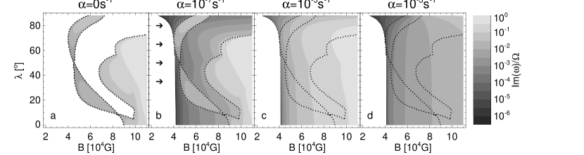
Figure 5: Growth rates of Parker-type and friction-induced instabilities of magnetic flux rings in the middle of the solar overshoot region. Shaded areas indicate unstable equilibria, with dotted lines marking boundaries of Parker-type instabilities in the frictionless case (panel a). Growth rates first increase with friction (panel b), then reach a maximum (panel c), and decrease for very strong friction (panel d). Arrows in panel b indicate the latitudes shown in Fig. 7.

The calculation of the $\mathcal{V}$-sequence confirms that the $\Delta_{6}$-criterion determines the onset of friction-induced instabilities (Fig. 6).

Figure 6: Sign changes of $\Delta_{4}$, $\Delta_{5}$, and $\Delta_{6}$ in the solar reference case, corresponding to the instability diagrams in Fig. 5. Tickmarks along each line indicate the downhill direction of the $\Delta_{k}$-functions. Within the shown range of field strengths and latitudes, $\Delta_{1-3}>0$.

For field strengths beyond this threshold, the sign change in the $\mathcal{V}$-sequence can occur at $\Delta_{5}$ or $\Delta_{4}$, but in the parameter range considered here there is always only one sign change, indicating a single unstable eigenmode. Given that the friction-induced instability sets in once an eigenmode reverses its propagation direction, the retrograde and prograde slow wave modes are liable to become unstable since the moduli of their phase velocities are smallest. Owing to the prograde plasma flow inside the flux tube, the retrograde wave is advected against its propagation direction and (the modulus of) its phase velocity closest to zero. In most cases it is the retrograde eigenmode which becomes frictionally unstable once its propagation reverses into prograde direction. An exception to this rule occurs if the threshold of the friction-induced instability coincides with strong driving caused by magnetic buoyancy. In the frictionless case, Parker-type instabilities are characterised by a merging of two eigenmodes: the phase velocities of both modes are identical and the growth rates of opposite sign (cf. Fig. 7, panel a).

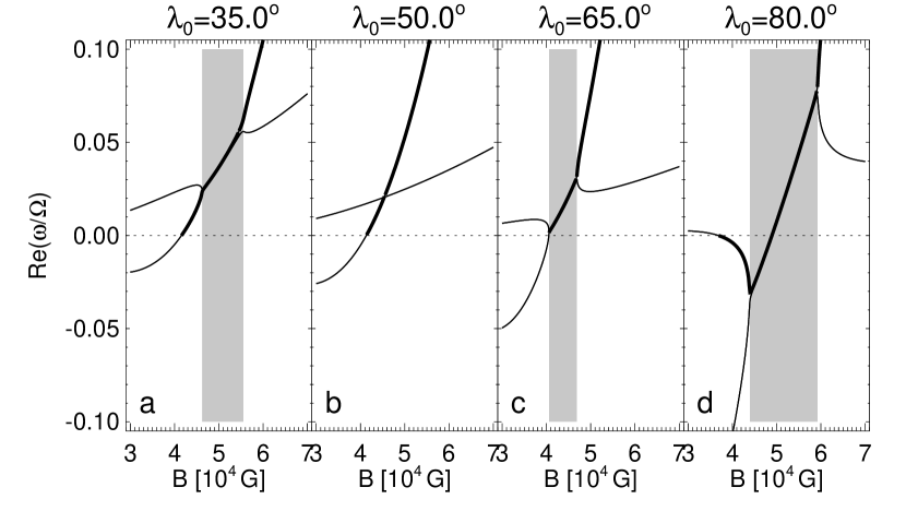
Figure 7: Oscillation frequencies of slow eigenmodes near to the threshold of friction-induced instabilities in the solar reference case. Each panel corresponds to a latitudinal cut in the stability diagram Fig. 5, panel b; the friction parameter is $\alpha=10^{-7}{\,{\rm s^{-1}}}$. Thick lines indicate an unstable eigenmode. In the gray shaded regions the instability is predominantly driven by magnetic buoyancy, outside by frictional coupling. Since the azimuthal wave number is $m=1$, we have $Re(\omega/\Omega)=v_{\scriptstyle\mathrm{ph}}/v_{\scriptstyle\mathrm{rot}}$.

If the merging coincides with the threshold of the friction-induced instability, the phase velocities of both eigenmodes are zero (panel c). In that situation, the prograde eigenmode can reverse its propagation to the retrograde direction and become frictionally unstable (panel d).

In contrast to the frictionless case, where magnetic flux rings at high latitudes may be stable up to high field strengths, flux rings subject to friction are generally unstable if their field strength is beyond the threshold given by Eq. (91). The growth rates depend on the dominating driving mechanisms, which in the parameter range considered here are frictional coupling and magnetic buoyancy; tension-driven poleward slip instabilities typically occur at higher field strengths. If friction is weak, growth rates are significant only if the flux tube equilibrium is in a parameter domain of Parker-type instabilities (Fig. 5, panel b). If friction is strong, a differentiation between Parker-stable and Parker-unstable domains becomes irrelevant, since the growth times are comparable. In case of very strong friction, growth rates decrease as flux tube motions are more and more harnessed by the environment.

4 Discussion

The criteria for friction-induced instability of straight and toroidal magnetic flux tubes are identical. From the equilibrium condition, Eq. (9) follows

$$Ro=\frac{2M_{\scriptstyle\mathrm{A}}^{2}}{1-M_{\scriptstyle\mathrm{A}}^{2}}\ ,$$ (93)

where $M_{\scriptstyle\mathrm{A}}=u_{0}/c_{\scriptstyle\mathrm{A}}$ is the Alfvénic Mach number, which is limited in the toroidal case to values $M_{\scriptstyle\mathrm{A}}<1$. Substitution of the Rossby number in the instability criterion, Eq. (88), yields

$$\omega_{\scriptstyle\mathrm{MBV}}^{2}<\left(\frac{c_{\scriptstyle\mathrm{A}}}{\gamma H_{\scriptstyle\mathrm{p}}}\right)^{2}\frac{1}{1-M_{\scriptstyle\mathrm{A}}^{2}}\ ,$$ (94)

which is the instability criterion of straight, horizontal flux tubes in the limit of long wavelengths (cf. Eq. (32) in 2007A&A...469...11H, ). In the limit of an infinite radius of curvature Eq. (94) becomes

$$\omega_{\scriptstyle\mathrm{MBV}}^{2}<\left(\frac{c_{\scriptstyle\mathrm{A}}}{\gamma H_{\scriptstyle\mathrm{p}}}\right)^{2}\quad\rightarrow\quad\beta\delta>-\frac{1}{\gamma}\ ,$$ (95)

since $u_{0}\rightarrow 0$ for $\kappa_{0}\rightarrow 0$. Relation (95) is the instability criterion of a straight flux tube in a stratified environment without a velocity difference between internal and external plasma (1982A&A...106...58S).

In contrast to the case of straight flux tubes, in which the flow velocity is a free parameter, the relative flow velocity inside toroidal flux tubes is fixed by the equilibrium condition. This implies an explicit dependence of the friction-induced instability on the curvature and field strength of the flux ring. The instability criterion, which relates the flow velocity with the phase velocity of a perturbation, thus determines a critical magnetic field strength (or, more general, Alfvén velocity) beyond which the friction-induced instability sets in. This critical field strength is lower than the threshold of the buoyancy-driven instability. A preliminary numerical parameter study indicates that this property applies to a broad range of stellar rotation rates and equilibrium depths in the overshoot region. From this, we conjecture that it is the friction-induced instability which determines whether flux ring equilibria in the overshoot region are stable or not.

Virtually all flux tube equilibria beyond the instability threshold are unstable. This is important, for example, in the case of fast stellar rotation. Stability analyses of flux rings in rapidly rotating stars (e.g. 1995GAFD...81..233; 2003A&A...405..291H) show that, in the frictionless case, for high magnetic field strengths isolated regions of stable equilibria exist, in which flux tubes are not subject to the Parker-type instability (see Fig. 8, panel a).

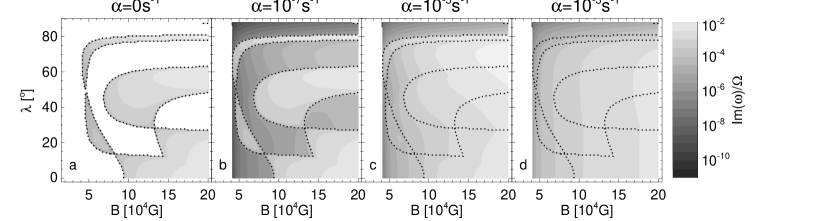
Figure 8: Like Fig. 5, but for a rapidly rotating star with a rotation period of $P_{\scriptstyle\mathrm{rot}}=2{\,{\rm d}}$. The Burger number is $Bu=8.04\cdot 10^{-5}$. In accordance with the results shown in Fig. 4, the latitude dependence of the threshold is weaker than in the solar reference case and only effective at very high latitudes.

These field strengths are well beyond the threshold of the friction-induced instability. Therefore, if friction is taken into account, these equilibria are unstable with high growth rates (Fig. 8, panels c and d).

The possibility to store magnetic flux in the overshoot region depends on the growth rate of the instabilities. An evaluation of the growth rates of friction-induced instabilities requires an estimate for the friction parameter $\alpha$. A comparison of drag force, Eq. (2), and friction force, Eq. (4), yields

$$\alpha\sim\frac{C_{\scriptstyle\mathrm{D}}}{\pi a}\left|\@vec{u}_{\scriptstyle\mathrm{rel,\perp}}\right|\ .$$ (96)

The friction parameter of a magnetic flux tube which gives rise to a small sunspot is estimated through non-linear numerical simulations (see 1995ApJ...441..886C, for a description of the code). With $B_{0}=10^{5}{\,{\rm G}},a_{0}=1000{\,{\rm km}}$ (i.e., $\Phi\simeq 3\cdot 10^{21}{\,{\rm Mx}}$) and $C_{\scriptstyle\mathrm{D}}=1$ we obtain $\alpha\sim 10^{-7}{\,{\rm s^{-1}}}$. The results of the stability analysis in Fig. 5 show that for this value of the friction parameter growth rates are several orders of magnitude lower than the rotation rate. Sunspot-producing flux tubes are thus hardly susceptible to friction-induced instabilities.

Thin magnetic flux tubes are weeded out of the overshoot region on shorter time scales than thick flux tubes, and should therefore occur more often. This agrees with the trend indicated by umbral areas observed on the Sun, which follow a log-normal distribution with small surface features being more numerous than large features (e.g. 2005A&A...443.1061B). If the higher number of small surface features is a consequence of higher friction-induced emergence rates, the dynamics and stability properties of thin magnetic flux tubes are dominated by friction. In that case, the latitudinal distribution of surface features may also depend on the size of the magnetic feature, since thinner flux tubes experience a stronger deflection to higher latitudes by meridional circulation (e.g. 2006MNRAS.369.1703H). The influence of meridional circulation would possibly be diluted by the action of convective motions on rising flux tubes. But since the former effect is systematic and the latter random, a discernable signature may persist in the latitudinal distribution. Even if thin flux tubes do not make it to the surface due to convective interaction, their susceptibility to friction-induced instabilities implies a decrease of magnetic flux in the overshoot region, which affects the budget and amplification of magnetic fields in the tachocline region.

The numerical results shown in Sect. 3.4 are based on magnetic flux rings located in the middle of the solar overshoot layer. Owing to the strong dependence of stability properties on the superadiabaticity, flux tubes located deeper in the overshoot region require significantly higher field strength to become buoyancy unstable. The friction-induced instability eases the need for very high field strengths, since its threshold is below the critical field strength of the buoyancy-driven instability. For example, a flux ring located in the equatorial plane close the radiative core, in an environment with $\delta=-10^{-4}$ ($N=3\cdot 10^{-5}{\,{\rm s^{-1}}}$), becomes frictionally unstable for field strengths above $3.5\cdot 10^{5}{\,{\rm G}}$, which is well below the critical field strength of the Parker-type instability at $6.2\cdot 10^{5}{\,{\rm G}}$.

The friction-induced instability of toroidal flux tubes is also relevant in other astrophysical contexts, such as in circumstellar accretion discs. Accretion of mass implies the transport of angular momentum to larger radii, which requires an efficient coupling of adjacent disc annuli. The coupling of Keplerian shear flow through weak magnetic fields gives rise to the magneto-rotational instability (MRI), which generates magnetic turbulence and efficiently increases the viscous coupling and angular momentum transport (1991ApJ...376..214B). The MRI requires a poloidal magnetic field and is independent of the toroidal field component. This axi-symmetric shear instability occurs for vertical wavelengths larger than a critical, field-dependent value, though growth rates and threshold are independent of field strength. It is an interesting possibility that the friction-induced instability of toroidal fields complements the MRI by supporting the radial magnetic coupling of a disc. Both instability mechanisms produce their highest growth rates on large length scales, yet the friction-induced instability does intrinsically not saturate at high field strengths as the MRI. However, it is unclear what mechanisms aside of Keplerian shear can produce the required velocity difference between the plasma inside and outside the flux tube.

1996A&A...308.1013S investigated the dynamics and evolution of small flux rings in an accretion disc, including the drag force caused by shear flows. If a flux ring is deformed by a strong shear flow, variations of the tension force and density contrast occur along the flux tube, which produce two loops rising vertically through the disc until they emerge into the disc corona. These investigations confirm the strong influence of the drag force on the dynamics of flux tubes with small minor tube radii, but they do not consider friction-induced instabilities. A stability analysis including the drag force would be possible, because there is a flow component perpendicular to the axis of the equilibrium flux tube. Since differential rotation has a significant influence on the stability properties of magnetic flux rings (e.g. 1995GAFD...81..233), it will be necessary to include the effect of shear flows and more general equilibrium conditions in the stability analysis of the friction-induced instability in the framework of accretion discs.

It is not clear to which extend the results based on a linear velocity dependence of friction carry over to the non-linear case. Given the $\alpha$-independence of the instability thresholds, the actual functional form of friction, that is, linear or quadratic, seems to be of secondary importance, provided that it is anti-parallel to the flow velocity perpendicular to the tube axis. Numerical simulations based on the drag force confirm the properties of friction-induced instability derived here. A detailed analysis of the non-linear case and parameter study is the topic of a forthcoming paper in this series.

5 Conclusion

The friction-induced instability determines the stability properties of flux rings at the bottom of the convection zone, as its threshold is at lower field strengths than those of buoyancy- and tension-driven instabilities. The stability properties depend on the magnetic field strength and on the magnetic flux. The threshold also depends on the location of the flux ring, since the toroidal geometry causes a connection between the instability criterion and the equilibrium condition. The analytical results confirm that a magnetic flux tube subject to friction becomes unstable when a backward wave occurs, that is, when an eigenmode reverses its direction of propagation. We expect that friction-induced instabilities are also relevant in other astrophysical contexts, such as the angular momentum transport in accretion discs.

Appendix A Linear perturbations

We summarise the expressions describing adiabatic perturbations of toroidal magnetic flux tubes in mechanical equilibrium. Their detailed derivation can be found, for example, in 1998GApFD..89...75S and 1995GAFD...81..233.

Small displacements, $\@vec{\xi}(s,t)=\left(\xi_{t},\xi_{n},\xi_{b}\right)$, of the flux tube from its equilibrium position change the tangential, normal, and binormal vectors, $\@vec{t},\@vec{n},\@vec{b}$, respectively, of the Frenet basis, the curvature, $\kappa$, the flow velocity, $u$, and the acceleration of the internal plasma:

$$\@vec{t}_{1} = \left(\xi_{n,s}+\kappa_{0}\xi_{t}\right)\@vec{n}_{0}+\xi_{b,s}\@vec{b}_{0}$$ (97)

$$\@vec{n}_{1} = -\left(\xi_{n,s}+\kappa_{0}\xi_{t}\right)\@vec{t}_{0}+\kappa_{0}^{-1}\xi_{b,ss}\@vec{b}_{0}$$ (98)

$$\@vec{b}_{1} = -\xi_{b,s}\@vec{t}_{0}-\kappa_{0}^{-1}\xi_{b,ss}\@vec{n}_{0}$$ (99)

$$\kappa_{1} = \xi_{n,ss}+\kappa_{0}^{2}\xi_{n}$$ (100)

$$\@vec{u}_{1} = \@vec{t}_{0}\left(\xi_{t,t}+u_{0}\xi_{t,s}-u_{0}\kappa_{0}\xi_{n}\right)$$ (101)

$${}+\@vec{n}_{0}\left(\xi_{n,t}+u_{0}\xi_{n,s}+u_{0}\kappa_{0}\xi_{t}\right)$$

$${}+\@vec{b}_{0}\left(\xi_{b,t}+u_{0}\xi_{b,s}\right)$$

$$\left(\frac{d}{dt}\@vec{u}\right)_{1} = \@vec{t}_{0}\left(\xi_{t,tt}+2u_{0}\xi_{t,st}-2u_{0}\kappa_{0}\xi_{n,t}+u_{0}^{2}\xi_{t,ss}\right.$$ (102)

$${}\left.\qquad-2u_{0}^{2}\kappa_{0}\xi_{n,s}-u_{0}^{2}\kappa_{0}^{2}\xi_{t}\right)$$

$${}+\@vec{n}_{0}\left(\xi_{n,tt}+2u_{0}\xi_{n,st}+2u_{0}\kappa_{0}\xi_{t,t}+2u_{0}^{2}\kappa_{0}\xi_{t,s}\right.$$

$${}\left.\qquad-u_{0}^{2}\kappa_{0}^{2}\xi_{n}+u_{0}^{2}\xi_{n,ss}\right)$$

$${}+\@vec{b}_{0}\left(\xi_{b,tt}+2u_{0}\xi_{b,st}+u_{0}^{2}\xi_{b,ss}\right)\ .$$

Quantities with index ’0’ and ’1’ are equilibrium and perturbed values, respectively, and indices ‘$,t$’ and ‘$,s$’ describe partial derivatives with respect to time, $t$, and equilibrium arclength, $s_{0}$.

The flux tube is in pressure equilibrium with its environment. Assuming adiabatic perturbations, the field strength, density, and density contrast, $\Delta\rho=\rho-\rho_{\scriptstyle\mathrm{e}}$, change according to the following equation:

$$\frac{B_{1}}{B_{0}} = \frac{\gamma\beta}{2+\gamma\beta}\frac{\left(\@vec{g}\cdot\@vec{\xi}\right)}{c_{\scriptstyle\mathrm{s,0}}^{2}}+\frac{\gamma\beta}{2+\gamma\beta}\left(\xi_{t,s}-\kappa_{0}\xi_{n}\right)$$ (103)

$$\frac{\rho_{1}}{\rho_{0}} = \frac{\gamma\beta}{2+\gamma\beta}\frac{\left(\@vec{g}\cdot\@vec{\xi}\right)}{c_{\scriptstyle\mathrm{s,0}}^{2}}-\frac{2}{2+\gamma\beta}\left(\xi_{t,s}-\kappa_{0}\xi_{n}\right)$$ (104)

$$\frac{\Delta\rho}{\rho}\bigg{|}_{1} = \frac{2}{\gamma\beta}\Delta\frac{\left(\@vec{g}\cdot\@vec{\xi}\right)}{c_{\scriptstyle\mathrm{s,0}}^{2}}-\frac{2}{2+\gamma\beta}\left(\xi_{t,s}-\kappa_{0}\xi_{n}\right)\ ,$$ (105)

with $\beta=8\pi p_{0}/B_{0}^{2}$ and

$$\Delta=\frac{\beta}{1+\beta}\left[\beta\delta-\frac{2}{\gamma}\left(\frac{1}{\gamma}-\frac{1}{2}\right)\frac{\gamma\beta}{2+\gamma\beta}\right]\ .$$ (106)

The superadiabaticity $\delta=\nabla-\nabla_{\scriptstyle\mathrm{ad}}$ quantifies the stability of the stratification against convective turnover ($\delta>0$: convectively unstable). From the integrated Walen equation, $\frac{B}{\rho}=\frac{B_{0}}{\rho_{0}}\frac{\partial s}{\partial s_{0}}$, follows

$$\left(\frac{1}{4\pi}\frac{B}{\rho}\frac{\partial}{\partial s}B\right)_{1}=\frac{B_{0}^{2}}{4\pi\rho_{0}}\left(\frac{B_{1}}{B_{0}}\right)_{,s}\ .$$ (107)

Appendix B Coefficients of dispersion polynomials

B.1 General case

Based on the linearised equations of motion in the form of Eq. (42), the eigenfrequencies of magnetic flux rings in mechanical equilibrium parallel to the equatorial plane are determined by the monic dispersion polynomial

$$\sum\limits_{j=0}^{6}c_{j}\tilde{\omega}^{j}=0\ ,$$ (108)

which stems from the coefficient matrix of Eq. (42). The coefficients are:

$$c_{5} = -6mRo+2i\tilde{\alpha}$$ (109)

$$c_{4} = 4\left(3m^{2}-1\right)Ro^{2}-2\left(3m^{2}+4\right)Ro-4$$ (110)

$${}-g_{\perp}^{2}\tilde{\omega}_{\scriptstyle\mathrm{MBV}}^{2}+2\frac{g_{\scriptstyle\mathrm{n}}}{\gamma f_{0}}\eta^{2}-8i\tilde{\alpha}mRo-\tilde{\alpha}^{2}$$

$$c_{3} = -8m\left(m^{2}-1\right)Ro^{3}+8m\left(3m^{2}+1\right)Ro^{2}$$ (111)

$${}+4mg_{\perp}^{2}\tilde{\omega}_{\scriptstyle\mathrm{MBV}}^{2}Ro-4m\frac{g_{\scriptstyle\mathrm{n}}}{\gamma f_{0}}\left(Ro-1\right)\eta^{2}$$

$${}+i\tilde{\alpha}\big{[}4\left(2m^{2}-1\right)Ro^{2}-8\left(m^{2}+1\right)Ro-4$$

$$\quad{}-g_{\perp}^{2}\tilde{\omega}_{\scriptstyle\mathrm{MBV}}^{2}+2\frac{g_{\scriptstyle\mathrm{n}}}{\gamma f_{0}}\eta^{2}\big{]}+2\tilde{\alpha}^{2}mRo$$

$$c_{2} = -24m^{2}\left(m^{2}-1\right)Ro^{3}+4m^{2}\left(3m^{2}+7\right)Ro^{2}+8m^{2}Ro$$ (112)

$${}-4\tilde{\omega}_{\scriptstyle\mathrm{MBV}}^{2}\big{[}g_{\perp}^{2}m^{2}\left(Ro-1\right)Ro-g_{\scriptstyle\mathrm{b}}^{2}\left(Ro+1\right)^{2}\big{]}$$

$${}-12m^{2}\frac{g_{\scriptstyle\mathrm{n}}}{\gamma f_{0}}Ro\eta^{2}-\left(\frac{1}{\gamma f_{0}}\right)^{2}\left(g_{\perp}^{2}m^{2}+g_{\scriptstyle\mathrm{b}}^{2}\right)\eta^{4}$$

$${}+2i\tilde{\alpha}m\big{[}4\left(2m^{2}-1\right)Ro^{2}-4Ro$$

$$\quad{}+g_{\perp}^{2}\tilde{\omega}_{\scriptstyle\mathrm{MBV}}^{2}Ro+2\frac{g_{\scriptstyle\mathrm{n}}}{\gamma f_{0}}\eta^{2}\big{]}+2\tilde{\alpha}^{2}m^{2}Ro$$

$$c_{1} = -24m^{3}\left(m^{2}-1\right)Ro^{3}+16m^{3}Ro^{2}$$ (113)

$${}-8m\tilde{\omega}_{\scriptstyle\mathrm{MBV}}^{2}\left[\left(g_{\perp}^{2}m^{2}-g_{\scriptstyle\mathrm{b}}^{2}\right)Ro-g_{\scriptstyle\mathrm{b}}^{2}\right]Ro$$

$${}-8m^{3}\frac{g_{\scriptstyle\mathrm{n}}}{\gamma f_{0}}Ro\eta^{2}+2m\left(\frac{1}{\gamma f_{0}}\right)^{2}\left[\left(g_{\perp}^{2}m^{2}-g_{\scriptstyle\mathrm{b}}^{2}\right)Ro-2g_{\scriptstyle\mathrm{b}}^{2}\right]\eta^{4}$$

$${}+i\tilde{\alpha}m^{2}\big{[}4\left(2m^{2}-1\right)Ro^{2}+2g_{\perp}^{2}\tilde{\omega}_{\scriptstyle\mathrm{MBV}}^{2}Ro-\left(\frac{g_{\perp}}{\gamma f_{0}}\right)^{2}\eta^{4}\big{]}$$

$$c_{0} = -8m^{4}\left(m^{2}-1\right)Ro^{3}$$ (114)

$${}-2m^{2}\left(g_{\perp}^{2}m^{2}-g_{\scriptstyle\mathrm{b}}^{2}\right)\left[2\tilde{\omega}_{\scriptstyle\mathrm{MBV}}^{2}Ro-\left(\frac{1}{\gamma f_{0}}\right)^{2}\eta^{4}\right]Ro$$

B.2 Axi-symmetric perturbations

In the special case of axial symmetric perturbations the dispersion equation reduces to the monic quartic polynomial in Eq. (45). The friction-independent part of the coefficients are:

$$c_{2} = 2\left(\frac{g_{\scriptstyle\mathrm{n}}}{\gamma f_{0}}-2\right)Ro\left(Ro+2\right)-4-g_{\perp}^{2}\,\tilde{\omega}_{\scriptstyle\mathrm{MBV}}^{2}$$ (115)

$$c_{0} = g_{\scriptstyle\mathrm{b}}^{2}\left(4\tilde{\omega}_{\scriptstyle\mathrm{MBV}}^{2}\left(Ro+1\right)^{2}-\left(\frac{1}{\gamma f_{0}}\right)^{2}Ro^{2}\left(Ro+2\right)^{2}\right)$$ (116)

B.3 Flux tubes in the equatorial plane

For flux rings in the equatorial plane the dispersion equation factorises in a quadratic and quartic polynomial, which describe the perturbation perpendicular and parallel to the equatorial plane, respectively. The coefficients of the latter are:

$$c_{3} = -4\,m\,Ro+i\,\tilde{\alpha}$$ (117)

$$c_{2} = 4\,\left(m^{2}-1\right)\,Ro^{2}-4\,\left(m^{2}+2\right)\,Ro-4$$ (118)

$${}-\tilde{\omega}_{\scriptstyle\mathrm{MBV}}^{2}\,g_{n}^{2}+2\,\frac{g_{n}}{\gamma f_{0}}\,\eta^{2}-2\,i\,\tilde{\alpha}\,m\,Ro$$

$$c_{1} = 8\,\left(m^{2}-1\right)\,m\,Ro^{2}-8\,m\,Ro$$ (119)

$${}+2\,m\,g_{\scriptstyle\mathrm{n}}^{2}\,\tilde{\omega}_{\scriptstyle\mathrm{MBV}}^{2}\,Ro+4\,m\,\frac{g_{\scriptstyle\mathrm{n}}}{\gamma f_{0}}\,\eta^{2}-2\,i\,\tilde{\alpha}\,m^{2}\,Ro$$

$$c_{0} = 4\,\left(m^{2}-1\right)\,m^{2}\,Ro^{2}$$ (120)

$${}+2\,m^{2}\,g_{\scriptstyle\mathrm{n}}^{2}\,\tilde{\omega}_{\scriptstyle\mathrm{MBV}}^{2}\,Ro-m^{2}\,\left(\frac{g_{\scriptstyle\mathrm{n}}}{\gamma f_{0}}\right)^{2}\,\eta^{4}$$