Helicity correlations of vector bosons

Abstract

We calculate the helicity and polarization correlation functions in the Einstein-Podolsky-Rosen-type experiments with relativistic vector bosons. We show that the linear polarization correlation function in the appriopriately chosen state in the massless limit is the same as the correlation function in the scalar two-photon state. We show also that the polarization correlation function violate the Clauser-Horne-Shimony-Holt inequality and that the degree of this violation can increase with the particle momentum.

I Introduction

Starting from Czachor’s paper Czachor (1997), Einstein-Podolsky-Rosen (EPR) correlations and other quantum information primitives in the relativistic context have been widely discussed Ahn et al. (2002, 2003a, 2003b); Alsing and Milburn (2002); Bartlett and Terno (2005); Caban and Rembieliński (2003, 2005, 2006); Czachor and Wilczewski (2003); Czachor (2005); Gingrich and Adami (2002); Gingrich et al. (2003); Gonera et al. (2004); Harshman (2005); Jordan et al. (2006a, b); Kosiński and Maślanka (2003); Kim and Son (2005); Li and Du (2003, 2004); Lamata et al. (2006); Lindner et al. (2003); Lee and Chang-Young (2004); Peres et al. (2002, 2005); Peres and Terno (2003a, b, 2004); Rembieliński and Smoliński (2002); Soo and Lin (2004); Terashima and Ueda (2003); You et al. (2004); Caban (2007); Caban et al. (2008). For massive particles mostly the spin degrees of freedom are considered. However, the definition of the spin operator for the relativistic particle is not unique and different operators have been used by different authors Czachor (1997); Terno (2003); Czachor and Wilczewski (2003); Lee and Chang-Young (2004); Czachor (2005); Caban and Rembieliński (2005).

On the other hand the helicity of the massive particle can be defined unambiguously and recent papers He et al. (2007, 2008); Shao et al. (2008) shows that helicity entanglement of fermion pair behaves in a different way than spin entanglement. Moreover, the carrier space of the irreducible, unitary representation of the Poincaré group for photons is spanned by helicity eingenstates. Furthermore, one can expect that the photon case can be received as a massless limit of the spin 1 boson case. In the recent paper Caban et al. (2008) the spin correlation function for the pair of vector bosons in the covariant framework have been discussed and the very surprising behavior of this function has been reported. In the center-of-mass frame for the definite configuration of the particles momenta and directions of the spin projection measurements this correlation function still depends on the value of the particle momentum and for some configurations this dependence is not monotonic. In other words, for fixed spin measurement directions and particle momenta directions, the spin correlation function can have an extremum.

Therefore, it is very interesting to consider helicity correlation function for the boson pair and the massless limit of this function. In this paper we calculate ordinary helicity correlation function of the boson pair in certain scalar states. However, for photons usually the polarization correlations are considered. Therefore, for massive vector bosons we also define polarization states and calculate polarization correlation function. In particular we identify the two-particle scalar state which posseses a proper massless limit, calculate polarization correlation function in this state, and show that the massless limit of this function is the same as the correlation function in the scalar two-photon state. We discuss also the violation of the Clauser-Horne-Shimony-Holt (CHSH) inequality by the polarization correlation function. We show that the degree of violation of the CHSH inequality in the center of mass frame depends on the particle momenta. What is very interesting, we find that the degree of violation of the CHSH inequality can increase with the particle momentum.

In Sec. II we recall basic facts concerning the massive spin 1 representations of the Poincaré group in the helicity basis. Section III is devoted to the discussion of states transforming covariantly with respect to the Poincaré group action. In Sec. IV we calculate explicitly helicity correlations of the boson pair in certain scalar states. In Sec. V we define states corresponding to the longitudal and transversal polarization of vector particle. In the next section we calculate polarization correlation function for the boson pair; we discuss also properties of this function and its massless limit. In this section we consider also the violation of Bell-type inequalities. The last section contains concluding remarks.

In the paper we use the natural units $\hbar=c=1$, the metric tensor $\eta^{\mu\nu}=\textrm{diag}(1,-1,-1,-1)$, and the antisymmetric tensor $\epsilon^{\alpha\beta\mu\nu}$ with $\epsilon^{0123}=1$.

II Representations of the Poincaré group in the helicity basis

In this section we recall the basic facts concerning the spin-1 representation of the Poincaré group in the helicity basis. Let $\mathcal{H}$ be the carrier space of the irreducible massive spin-1 representation of the Poincaré group. The spin basis of the space $\mathcal{H}$ we denote by $\{|p,\sigma\rangle\}_{\sigma=0,\pm 1}$ while the helicity basis by $\{|p,\lambda\rangle\}_{\lambda=0,\pm 1}$. Vectors $|p,\sigma\rangle$ are eigenvectors of the four-momentum operators

$$\hat{P}^{\mu}|p,\sigma\rangle=p^{\mu}|p,\sigma\rangle,$$ (1)

where $p^{2}=m^{2}$ and $m$ is the mass of the particle. We use the Lorentz-covariant normalization of the spin basis vectors

$$\langle p,\sigma|p^{\prime},\sigma^{\prime}\rangle=2p^{0}\delta^{3}(\textbf{p}-\textbf{p}^{\prime})\delta_{\sigma\sigma^{\prime}}.$$ (2)

The vectors $|p,\sigma\rangle$ can be generated from standard vector $|\tilde{p},\sigma\rangle$, where $\tilde{p}=m(1,0,0,0)$. We have $|p,\sigma\rangle=U(L_{p})|\tilde{p},\sigma\rangle$, where Lorentz boost $L_{p}$ is defined by relations $p=L_{p}\tilde{p}$, $L_{\tilde{p}}=\operatorname{\openone}$, and its explicit form is

$$L_{p}=\left(\begin{array}[]{c|c}\tfrac{p^{0}}{m}&\tfrac{\textbf{p}^{T}}{m}\\ \hline\cr\tfrac{\textbf{p}}{m}&\operatorname{\openone}+\tfrac{\textbf{p}\otimes\textbf{p}^{T}}{m(m+p^{0})}\end{array}\right),$$ (3)

where $p^{0}=\sqrt{m^{2}+\textbf{p}^{2}}$.

The standard Wigner induction procedure gives

$$U(\Lambda)|p,\sigma\rangle=\mathcal{D}_{\sigma^{\prime}\sigma}(R(\Lambda,p))|\Lambda p,\sigma^{\prime}\rangle,$$ (4)

where the Wigner rotation $R(\Lambda,p)$ is defined as $R(\Lambda,p)=L_{\Lambda p}^{-1}\Lambda L_{p}$ and $\mathcal{D}(R)$ is the standard spin-1 representation of the rotation group. $3\times 3$ matrix representations of the rotation group, $\mathcal{D}(R)$ and $R$, are unitary equivalent, i.e. for every rotation $R$

$$\mathcal{D}(R)=VRV^{{\dagger}},$$ (5)

where

$$V=\frac{1}{\sqrt{2}}\left(\begin{array}[]{ccc}-1&i&0\\ 0&0&\sqrt{2}\\ 1&i&0\\ \end{array}\right)$$ (6)

(see Caban et al. (2008)).

The helicity basis vectors $|p,\lambda\rangle$ are connected with the spin basis vectors $|p,\sigma\rangle$ via the relation Weinberg (1964):

$$|p,\lambda\rangle=\mathcal{D}_{\sigma\lambda}(R_{p})|p,\sigma\rangle,$$ (7)

where $R_{p}$ denotes the rotation which rotates the $z$-axis on the direction of the vector p, i.e.:

$$R_{p}\begin{pmatrix}0\\ 0\\ 1\end{pmatrix}=\textbf{n}_{\textbf{p}}\equiv\frac{\textbf{p}}{|\textbf{p}|}.$$ (8)

The most general form of the rotation $R_{p}$ is

$$R_{p}=\left(\textbf{a}_{\textbf{p}}\Big{|}\textbf{n}_{\textbf{p}}\times\textbf{a}_{\textbf{p}}\Big{|}\textbf{n}_{\textbf{p}}\right),$$ (9)

where $|\textbf{a}_{\textbf{p}}|=1$, $\textbf{a}_{\textbf{p}}\perp\textbf{n}_{\textbf{p}}$ and we treat vectors in (9) as column matrices. Vectors $|p,\lambda\rangle$ are eigenvectors of the four-momentum operators

$$\hat{P}^{\mu}|p,\lambda\rangle=p^{\mu}|p,\lambda\rangle,$$ (10)

and Eqs. (2), (7) imply the Lorentz-covariant normalization of the helicity basis

$$\langle p,\lambda|p^{\prime},\lambda^{\prime}\rangle=2p^{0}\delta^{3}(\textbf{p}-\textbf{p}^{\prime})\delta_{\lambda\lambda^{\prime}}.$$ (11)

Vectors $|p,\lambda\rangle$ are eigenvectors of the helicity operator

$$\frac{\textbf{J}\cdot\textbf{P}}{|\textbf{P}|}|p,\lambda\rangle=\lambda|p,\lambda\rangle,$$ (12)

where $\textbf{J}=(J_{1},J_{2},J_{3})$, $J_{i}=\frac{1}{2}\varepsilon_{ijk}J_{ij}$ and $J_{\mu\nu}$ denote the generators of the Lorentz group such that $U(\Lambda)=\exp(i\omega^{\mu\nu}J_{\mu\nu})$. Let us note that $\textbf{J}\cdot\textbf{P}=W^{0}$, where the Pauli-Lubanski four-vector is defined as

$$W^{\mu}=\tfrac{1}{2}\epsilon^{\nu\alpha\beta\mu}P_{\nu}J_{\alpha\beta}.$$ (13)

The relation (7) can be inverted

$$|p,\sigma\rangle=\mathcal{D}_{\lambda\sigma}(R_{p}^{-1})|p,\lambda\rangle.$$ (14)

Now, from Eqs. (4), (7), and (14) we have

$$U(\Lambda)|p,\lambda\rangle=\mathcal{D}_{\lambda^{\prime}\lambda}(R_{\Lambda p}^{-1}R(\Lambda,p)R_{p})|\Lambda p,\lambda^{\prime}\rangle.$$ (15)

III Covariant states

Now, following Caban et al. (2008), let us define states

$$|(\mu,p)\rangle=e^{\mu}_{\phantom{\mu}\sigma}(p)|p,\sigma\rangle,$$ (16)

which transform covariantly

$$U(\Lambda)|(\mu,p)\rangle=(\Lambda^{-1})^{\mu}_{\phantom{\mu}\nu}|(\nu,\Lambda p)\rangle.$$ (17)

In Eq. (16) $e_{\phantom{\mu}\sigma}^{\mu}(p)$ denotes the vector boson field amplitudes (see Caban et al. (2008) for the details). Consistency of Eqs. (4), (16), and (17) is guaranteed by the Weinberg condition Caban et al. (2008)

$$e^{\mu}_{\phantom{\mu}\sigma}(\Lambda p)=\Lambda^{\mu}_{\phantom{\mu}\nu}e^{\nu}_{\phantom{\nu}\sigma^{\prime}}(p)\mathcal{D}(R(\Lambda,p))_{\sigma\sigma^{\prime}}.$$ (18)

The explicit form of the amplitudes $e_{\phantom{\mu}\sigma}^{\mu}(p)$ can be determined from Eq. (18) (see Caban et al. (2008))

$$e(p)=\left(\begin{array}[]{c}\tfrac{\textbf{p}^{T}}{m}\\ \hline\cr\operatorname{\openone}+\tfrac{\textbf{p}\otimes\textbf{p}^{T}}{m(m+p^{0})}\end{array}\right)V^{\mathrm{T}}.$$ (19)

Moreover, amplitudes (19) fulfil the following conditions:

$$p_{\mu}e^{\mu}_{\phantom{\mu}\sigma}(p)=0,$$ (20a)

$$e^{*\mu}_{\phantom{*\mu}\sigma}(p)e_{\mu\sigma^{\prime}}(p)=-\delta_{\sigma\sigma^{\prime}},$$ (20b)

$$e^{\mu}_{\phantom{\mu}\sigma}(p)e_{\mu\sigma^{\prime}}(p)=-(VV^{\mathrm{T}})_{\sigma\sigma^{\prime}},$$ (20c)

$$e^{*\mu}_{\phantom{*\mu}\sigma}(p)e^{\nu}_{\phantom{\nu}\sigma}(p)=-\eta^{\mu\nu}+\tfrac{p^{\mu}p^{\nu}}{m^{2}},$$ (20d)

where $e(p)VV^{\mathrm{T}}=e^{*}(p)$, and $VV^{\mathrm{T}}=\left(\begin{array}[]{ccc}0&0&-1\\ 0&1&0\\ -1&0&0\\ \end{array}\right)$.

The covariant states (16) are normalized as follows [c.f. Eq. (2)]

$$\langle(\mu,p^{\prime})|(\nu,p)\rangle=2p^{0}\delta^{3}(\textbf{p}^{\prime}-\textbf{p})e^{*\mu}_{\phantom{*\mu}\sigma}(p^{\prime})e^{\nu}_{\phantom{\nu}\sigma}(p).$$ (21)

Using helicity basis we have

$$|(\mu,p)\rangle=e^{\mu}_{\phantom{\mu}\sigma}(p){\mathcal{D}}_{\lambda\sigma}(R_{p}^{-1})|p,\lambda\rangle\equiv E^{\mu}_{\phantom{\mu}\lambda}(p)|p,\lambda\rangle.$$ (22)

Equations (5), (19), and (20) imply

$$p_{\mu}E^{\mu}_{\phantom{\mu}\lambda}(p)=0,$$ (23a)

$$E^{*\mu}_{\phantom{*\mu}\lambda}(p)E_{\mu\lambda^{\prime}}(p)=-\delta_{\lambda\lambda^{\prime}},$$ (23b)

$$E^{\mu}_{\phantom{\mu}\lambda}(p)E_{\mu\lambda^{\prime}}(p)=-(VV^{T})_{\lambda\lambda^{\prime}},$$ (23c)

$$E^{*\mu}_{\phantom{*\mu}\lambda}(p)E^{\nu}_{\phantom{\nu}\lambda}(p)=-\eta^{\mu\nu}+\frac{p^{\mu}p^{\nu}}{m^{2}},$$ (23d)

and

$$E(p)=\left(\begin{array}[]{c}\tfrac{\textbf{p}^{T}}{m}\\ \hline\cr\operatorname{\openone}+\tfrac{\textbf{p}\otimes\textbf{p}^{T}}{m(m+p^{0})}\end{array}\right)R_{p}V^{\mathrm{T}}.$$ (24)

Thus, applying Eqs. (6), (9), and (24) we have explicitly

$$E(p)=\left(\begin{array}[]{c|c|c}0&\frac{\textbf{p}^{2}}{m|\textbf{p}|}&0\\ \hline\cr\frac{-\textbf{a}_{\textbf{p}}+i(\textbf{n}_{\textbf{p}}\times\textbf{a}_{\textbf{p}})}{\sqrt{2}}&\frac{p^{0}\textbf{p}}{m|\textbf{p}|}&\frac{\textbf{a}_{\textbf{p}}+i(\textbf{n}_{\textbf{p}}\times\textbf{a}_{\textbf{p}})}{\sqrt{2}}\end{array}\right),$$ (25)

where the first column of the above matrix corresponds to $\lambda=1$, the second one to $\lambda=0$, and the third one to $\lambda=-1$. For futher convenience let us introduce the following notation

$$|(k,\lambda);(p,\lambda^{\prime})\rangle\equiv\frac{1}{\sqrt{2}}\big{[}|k,\lambda\rangle\otimes|p,\lambda^{\prime}\rangle+|p,\lambda^{\prime}\rangle\otimes|k,\lambda\rangle\big{]}.$$ (26)

For $k\not=p$ Eq. (11) imply

$$\langle(k,\tau);(p,\tau^{\prime})|(k,\lambda);(p,\lambda^{\prime})\rangle=4k^{0}p^{0}\big{[}\delta^{3}(\textbf{0})\big{]}^{2}\delta_{\tau\lambda}\delta_{\tau^{\prime}\lambda^{\prime}}.$$ (27)

Finally, with help of one-particle covariant states (16), we can define two-particle states which posses defined transformation properties under Lorentz group action. In particular, the most general scalar state with sharp momenta has the following form:

$$|\chi(k,p)\rangle=\alpha(k,p)(kp)|\psi(k,p)\rangle+\beta(k,p)|\phi(k,p)\rangle,$$ (28)

where two independent scalar states, $|\psi(k,p)\rangle$ and $|\phi(k,p)\rangle$, are given by

$$|\psi(k,p)\rangle =\eta_{\mu\nu}E^{\mu}_{\phantom{\mu}\lambda}(k)E^{\nu}_{\phantom{\nu}\lambda^{\prime}}(p)|(k,\lambda);(p,\lambda^{\prime})\rangle,$$ (29)

$$|\phi(k,p)\rangle =\big{[}p_{\mu}E^{\mu}_{\phantom{\mu}\lambda}(k)\big{]}\big{[}k_{\nu}E^{\nu}_{\phantom{\nu}\lambda^{\prime}}(p)\big{]}|(k,\lambda);(p,\lambda^{\prime})\rangle,$$ (30)

and $\alpha(k,p)$, $\beta(k,p)$ denote scalar functions of four-momenta $k$ and $p$. In the EPR-type experiments Alice and Bob measure correlation function in the two-particle state with different momenta. Therefore, in the rest of the paper we will assume that in the states (29), (30) $k\not=p$. In this case it holds

$$\langle\psi(k,p)|\psi(k,p)\rangle =4k^{0}p^{0}\big{[}\delta^{3}(\textbf{0})\big{]}^{2}\Big{[}\frac{(kp)^{2}}{m^{4}}+2\Big{]},$$ (31)

$$\langle\phi(k,p)|\phi(k,p)\rangle =4k^{0}p^{0}\big{[}\delta^{3}(\textbf{0})\big{]}^{2}m^{4}\Big{[}\frac{(kp)^{2}}{m^{4}}-1\Big{]}^{2},$$ (32)

$$\langle\phi(k,p)|\psi(k,p)\rangle =4k^{0}p^{0}\big{[}\delta^{3}(\textbf{0})\big{]}^{2}(kp)\Big{[}\frac{(kp)^{2}}{m^{4}}-1\Big{]}.$$ (33)

With help of the above equations we can easily find the square of the norm of the state $|\chi(k,p)\rangle$

$$\langle\chi(k,p)|\chi(k,p)\rangle=4k^{0}p^{0}\big{[}\delta^{3}(\textbf{0})\big{]}^{2}\\ \times\Big{\{}|\alpha|^{2}(kp)^{2}\Big{[}\frac{(kp)^{2}}{m^{4}}+2\Big{]}+|\beta|^{2}m^{4}\Big{[}\frac{(kp)^{2}}{m^{4}}-1\Big{]}^{2}+\\ +(\alpha^{*}\beta+\alpha\beta^{*})(kp)^{2}\Big{[}\frac{(kp)^{2}}{m^{4}}-1\Big{]}\Big{\}}.$$ (34)

In the discussion of the massless limit of the correlation function, the following state will be of special interest

$$|\xi(k,p)\rangle=-(kp)|\psi(k,p)\rangle+|\phi(k,p)\rangle.$$ (35)

For the state (35) it holds

$$\langle\xi(k,p)|\xi(k,p)\rangle=4k^{0}p^{0}\big{[}\delta^{3}(\textbf{0})\big{]}^{2}\Big{[}2(kp)^{2}+m^{4}\Big{]}.$$ (36)

IV Helicity correlations

Now, we will calculate helicity correlations in the EPR type experiments. We assume that Alice and Bob share two-particle scalar state defined in Eq. (28) (with $k\not=p$) and Alice measures the helicity of the particle with the four-momentum $k$ and Bob the helicity of the particle with the four-momentum $p$. Therefore, Alice uses the observable

$$\Lambda_{k}=\hat{\lambda}_{k}\otimes\openone+\openone\otimes\hat{\lambda}_{k},$$ (37)

where

$$\hat{\lambda}_{k}|k,\lambda\rangle=\lambda|k,\lambda\rangle,$$ (38)

and

$$\hat{\lambda}_{k}|p,\lambda\rangle=0,\quad k\not=p;$$ (39)

while Bob uses the observable

$$\Lambda_{p}=\hat{\lambda}_{p}\otimes\openone+\openone\otimes\hat{\lambda}_{p}.$$ (40)

$\hat{\lambda}_{p}$ fulfills relations analogous to Eqs. (38) and (39). Helicity correlation function has the form

$$\mathcal{C}_{\textsf{helicity}}^{\chi(k,p)}(k,p)=\frac{\langle\chi(k,p)|\Lambda_{p}\Lambda_{k}|\chi(k,p)\rangle}{\langle\chi(k,p)|\chi(k,p)\rangle}.$$ (41)

Taking into account Eqs. (24), (29), (30), and (27) after strightforward calculation, we receive

$$\langle\psi(k,p)|\Lambda_{p}\Lambda_{k}|\psi(k,p)\rangle =-8k^{0}p^{0}\big{[}\delta^{3}(\textbf{0})\big{]}^{2}\frac{\textbf{k}\cdot\textbf{p}}{|\textbf{k}||\textbf{p}|},$$ (42a)

$$\langle\phi(k,p)|\Lambda_{p}\Lambda_{k}|\phi(k,p)\rangle =0,$$ (42b)

$$\langle\phi(k,p)|\Lambda_{p}\Lambda_{k}|\psi(k,p)\rangle =-k^{0}p^{0}\big{[}\delta^{3}(\textbf{0})\big{]}^{2}\frac{(\textbf{k}\times\textbf{p})^{2}}{|\textbf{k}||\textbf{p}|}.$$ (42c)

Now, using Eqs. (28), (34), and (42) one can easily calculate correlation function (41) for arbitrary state $|\chi(k,p)\rangle$. We give here explicit formulas for some special cases. First of all, Eq. (42b) imply that for the state (30) we have

$$\mathcal{C}_{\textsf{helicity}}^{\phi(k,p)}(k,p)=0.$$ (43)

For the state (29) we have

$$\mathcal{C}_{\textsf{helicity}}^{\psi(k,p)}(k,p)=-\frac{2}{\big{[}2+\frac{(kp)^{2}}{m^{4}}\big{]}}\frac{\textbf{k}\textbf{p}}{|\textbf{k}||\textbf{p}|}.$$ (44)

It should be noted that the standard spin correlation function in the EPR-type expiriment in which Alice and Bob share the state (29) and measure the spin components in directions a and b, respectively, was calculated in Ref. Caban et al. (2008). This function has the following form Caban et al. (2008):

$$\mathcal{C}_{\textsf{spin}}^{\psi(k,p)}(k,\textbf{a};p,\textbf{b})=\frac{2}{m^{2}\big{[}2+\frac{(kp)^{2}}{m^{4}}\big{]}}\Big{\{}-(\textbf{a}\cdot\textbf{b})(kp)+\\ -(\textbf{a}\cdot\textbf{p})(\textbf{b}\cdot\textbf{k})-\frac{(\textbf{a}\cdot\textbf{k})(\textbf{b}\cdot\textbf{p})(\textbf{k}\cdot\textbf{p})}{(m+k^{0})(m+p^{0})}+\\ +\frac{k^{0}(\textbf{a}\cdot\textbf{p})(\textbf{b}\cdot\textbf{p})}{m+p^{0}}+\frac{p^{0}(\textbf{a}\cdot\textbf{k})(\textbf{b}\cdot\textbf{k})}{m+k^{0}}\Big{\}}.$$ (45)

In Caban et al. (2008) the following relativistic spin operator

$$\textbf{S}=\frac{1}{m}\left(\textbf{W}-W^{0}\frac{\textbf{P}}{P^{0}+m}\right),$$ (46)

has been used. For this operator it holds $\textbf{S}\cdot\textbf{P}=W^{0}$. Therefore, we can write

$$\frac{\textbf{S}\cdot\textbf{P}}{|\textbf{P}|}|p,\lambda\rangle=\lambda|p,\lambda\rangle.$$ (47)

Thus, one can expect that choosing directions of Alice’s and Bob’s measurements parallel to k and p, respectively, i.e. putting in Eq. (45)

$$\textbf{a}=\frac{\textbf{k}}{|\textbf{k}|},\quad\textbf{b}=\frac{\textbf{p}}{|\textbf{p}|},$$ (48)

one should receive Eq. (44). Simple calculation shows that this is really the case.

Finally, helicity correlation function in the state (35) has the form

$$\mathcal{C}_{\textsf{helicity}}^{\xi(k,p)}(k,p)=\frac{-2(kp)}{2(kp)^{2}+m^{4}}\frac{(kp)(\textbf{k}\cdot\textbf{p})-(\textbf{k}\times\textbf{p})^{2}}{|\textbf{k}||\textbf{p}|}.$$ (49)

V Polarization states

Now, we define vectors describing polarized states

$$|\boldsymbol{\varepsilon}(p),p\rangle=\varepsilon_{\mu}(p)|(\mu,p)\rangle=\varepsilon_{\mu}(p)E^{\mu}_{\phantom{\mu}\lambda}(p)|p,\lambda\rangle.$$ (50)

It should be noted that without loss of generality we can assume

$$\varepsilon_{\mu}(p)p^{\mu}=0,$$ (51)

what is a consequence of Eq. (23a). Vectors (50) are normalized as follows:

$$\langle\boldsymbol{\varepsilon}(p),p|\boldsymbol{\varepsilon}^{\prime}(p^{\prime}),p^{\prime}\rangle=-2p^{0}\delta^{3}(\textbf{p}-\textbf{p}^{\prime})\varepsilon_{\phantom{*}\mu}^{*}(p)\varepsilon^{\prime\mu}(p).$$ (52)

V.1 Longitudal polarization

We say that vector (50) describes longitudal polarization, when $\boldsymbol{\varepsilon}(p)||\textbf{p}$. Therefore, using Eqs. (23a), (24), and (6), (8) one can easily show that

$$|\boldsymbol{\varepsilon}_{||}(p),p\rangle=|p,0\rangle,$$ (53)

and the corresponding polarization vector has the form

$$\boldsymbol{\varepsilon}_{||}(p)^{\mu}=-\Big{(}\frac{|\textbf{p}|}{m},\frac{p^{0}}{m|\textbf{p}|}\textbf{p}\Big{)}.$$ (54)

In Eq. (53) $|p,0\rangle$ denotes state with helicity 0.

V.2 Transversal polarization

Transversally polarized state is described by the vector (50) with polarization vector $\boldsymbol{\varepsilon}_{\perp}(p)$ orthogonal to the momentum p. This condition and Eqs. (23a, 24, 6, 8) imply

$$|\boldsymbol{\varepsilon}_{\perp}(p),p\rangle=\alpha|p,1\rangle+\beta|p,-1\rangle,$$ (55)

where $|\alpha|^{2}+|\beta|^{2}=1$, $|p,\pm 1\rangle$ are helicity states, and

$$\varepsilon_{\perp}(p)^{0}=0,$$ (56)

$$\boldsymbol{\varepsilon}_{\perp}(p)=\frac{1}{\sqrt{2}}\Big{[}(\alpha-\beta)\textbf{a}_{\textbf{p}}+i(\alpha+\beta)(\textbf{n}_{\textbf{p}}\times\textbf{a}_{\textbf{p}})\Big{]}.$$ (57)

States (55) are normalized according to [compare Eq. (52)]

$$\langle\boldsymbol{\varepsilon}_{\perp}(p),p|\boldsymbol{\varepsilon}_{\perp}^{\prime}(p^{\prime}),p^{\prime}\rangle=2p^{0}\delta^{3}(\textbf{p}-\textbf{p}^{\prime})\boldsymbol{\varepsilon}_{\perp}^{*}(p)\cdot\boldsymbol{\varepsilon}_{\perp}^{\prime}(p).$$ (58)

V.3 Circular and linear polarization

Circularly polarized states we recive from Eq. (55) putting $\alpha=1$, $\beta=0$ or $\alpha=0$, $\beta=1$

$$|\boldsymbol{\varepsilon}_{\perp}^{+}(p),p\rangle=|p,1\rangle,$$ (59)

$$|\boldsymbol{\varepsilon}_{\perp}^{-}(p),p\rangle=|p,-1\rangle.$$ (60)

Linearly polarized states we define in a standard way

$$|\boldsymbol{\varepsilon}_{\theta}(p),p\rangle =\frac{1}{\sqrt{2}}\big{[}e^{i\theta}|\boldsymbol{\varepsilon}_{\perp}^{+}(p),p\rangle+e^{-i\theta}|\boldsymbol{\varepsilon}_{\perp}^{-}(p),p\rangle\big{]}$$ (61)

$$=\frac{1}{\sqrt{2}}\big{[}e^{i\theta}|p,1\rangle+e^{-i\theta}|p,-1\rangle\big{]}.$$ (62)

Therefore the polarization vector for the linearly polarized state has the form

$$\boldsymbol{\varepsilon}_{\theta}(p)=i\Big{[}\sin{\theta}\textbf{a}_{\textbf{p}}+\cos{\theta}(\textbf{n}_{\textbf{p}}\times\textbf{a}_{\textbf{p}})\Big{]}.$$ (63)

States (62) are normalized as follows

$$\langle\boldsymbol{\varepsilon}_{\theta}(p),p|\boldsymbol{\varepsilon}_{\theta^{\prime}}(p^{\prime}),p^{\prime}\rangle=2p^{0}\delta^{3}(\textbf{p}-\textbf{p}^{\prime})\cos{(\theta-\theta^{\prime})}.$$ (64)

VI Linear polarization correlations

In this section we will consider EPR-type experiment in which Alice and Bob measure linear polarization of vector particles. Precisely, we assume that Alice and Bob share two-particle scalar state, particle with four-momentum $k$ flies to Alice, and particle with four-momentum $p$ flies to Bob. Alice (Bob) measures an observable which gives $+1$ when acting on boson with four-momentum $k$ ($p$), polarized linearly under the angle $\theta$ ($\tilde{\theta}$), and $-1$ for the similar boson polarized under the angle $\theta_{\perp}=\theta+\pi/2$ ($\tilde{\theta}_{\perp}$). Therefore, the observables used by Alice and Bob have the following form:

$$S^{\theta}_{k} =\Pi^{\theta}_{k}-\Pi^{\theta_{\perp}}_{k},$$ (65a)

$$S^{\tilde{\theta}}_{p} =\Pi^{\tilde{\theta}}_{p}-\Pi^{\tilde{\theta}_{\perp}}_{p},$$ (65b)

where

$$\Pi^{\theta}_{k}=\frac{1}{2k^{0}\delta^{3}(\textbf{0})}\Big{[}|\boldsymbol{\varepsilon}_{\theta}(k),k\rangle\langle\boldsymbol{\varepsilon}_{\theta}(k),k|\otimes\openone\\ +\openone\otimes|\boldsymbol{\varepsilon}_{\theta}(k),k\rangle\langle\boldsymbol{\varepsilon}_{\theta}(k),k|\Big{]},$$ (66)

and projectors $\Pi^{\theta_{\perp}}_{k}$, $\Pi^{\tilde{\theta}}_{p}$, $\Pi^{\tilde{\theta}_{\perp}}_{p}$ are defined analogously to $\Pi^{\theta}_{k}$. It should be noted that observables (65) commute

$$[S^{\theta}_{k},S^{\tilde{\theta}}_{p}]=0,$$ (67)

therefore the correlation function in the scalar state (28) has the form

$$\mathcal{C}^{\chi(k,p)}_{\textsf{polarization}}(k,\theta;p,\tilde{\theta})=\frac{\langle\chi(k,p)|S^{\tilde{\theta}}_{p}S^{\theta}_{k}|\chi(k,p)\rangle}{\langle\chi(k,p)|\chi(k,p)\rangle}.$$ (68)

The numerator of the right side of Eq. (68) can be written as [see Eqs. (65)]

$$\langle\chi(k,p)|S^{\tilde{\theta}}_{p}S^{\theta}_{k}|\chi(k,p)\rangle =\langle\chi(k,p)|\Pi^{\tilde{\theta}}_{p}\Pi^{\theta}_{k}|\chi(k,p)\rangle$$

$$+\langle\chi(k,p)|\Pi^{\tilde{\theta}_{\perp}}_{p}\Pi^{\theta_{\perp}}_{k}|\chi(k,p)\rangle$$

$$-\langle\chi(k,p)|\Pi^{\tilde{\theta}_{\perp}}_{p}\Pi^{\theta}_{k}|\chi(k,p)\rangle$$

$$-\langle\chi(k,p)|\Pi^{\tilde{\theta}}_{p}\Pi^{\theta_{\perp}}_{k}|\chi(k,p)\rangle.$$ (69)

It is enough to calculate explicitly only $\langle\chi(k,p)|\Pi^{\tilde{\theta}}_{p}\Pi^{\theta}_{k}|\chi(k,p)\rangle$, other terms on the right side of Eq. (69) can be received by appriopriate change of angles $\theta$ and/or $\tilde{\theta}$. Now, with help of Eqs. (22), (24), (29), (30), and (63) we find

$$\langle\psi(k,p)|\Pi^{\tilde{\theta}}_{p}\Pi^{\theta}_{k}|\psi(k,p)\rangle =4k^{0}p^{0}\big{[}\delta^{3}(\textbf{0})\big{]}^{2}\big{[}\boldsymbol{\varepsilon}_{\theta}(k)\cdot\boldsymbol{\varepsilon}_{\tilde{\theta}}(p)\big{]}^{2},$$ (70a)

$$\langle\phi(k,p)|\Pi^{\tilde{\theta}}_{p}\Pi^{\theta}_{k}|\phi(k,p)\rangle =4k^{0}p^{0}\big{[}\delta^{3}(\textbf{0})\big{]}^{2}\big{[}\textbf{p}\cdot\boldsymbol{\varepsilon}_{\theta}(k)\big{]}^{2}$$

$$\times\big{[}\textbf{k}\cdot\boldsymbol{\varepsilon}_{\tilde{\theta}}(p)\big{]}^{2},$$ (70b)

$$\langle\phi(k,p)|\Pi^{\tilde{\theta}}_{p}\Pi^{\theta}_{k}|\psi(k,p)\rangle =-4k^{0}p^{0}\big{[}\delta^{3}(\textbf{0})\big{]}^{2}\big{[}\textbf{p}\cdot\boldsymbol{\varepsilon}_{\theta}(k)\big{]}$$

$$\times\big{[}\textbf{k}\cdot\boldsymbol{\varepsilon}_{\tilde{\theta}}(p)\big{]}\big{[}\boldsymbol{\varepsilon}_{\theta}(k)\cdot\boldsymbol{\varepsilon}_{\tilde{\theta}}(p)\big{]}.$$ (70c)

Using above formulas one can calculate explicitly $\langle\chi(k,p)|\Pi^{\tilde{\theta}}_{p}\Pi^{\theta}_{k}|\chi(k,p)\rangle$ for arbitrary choice of functions $\alpha(k,p)$ and $\beta(k,p)$ in the state $|\chi(k,p)\rangle$ [see Eq. (28)]. Thus, with help of Eqs. (69), and (70) and the normalization (34), the correlation function (68) can be easily calculated for arbitrary scalar state $|\chi(k,p)\rangle$. However, the resulting general formula appears to be rather long and we do not put it here. Instead of that we will concentrate on some special cases. First of all, correlation functions in the states $|\psi(k,p)\rangle$ [Eq. (29)] and $|\phi(k,p)\rangle$ [Eq. (30)] have the following form:

$$\mathcal{C}^{\psi(k,p)}_{\textsf{polarization}}(k,\theta;p,\tilde{\theta})=\frac{1}{2+\frac{(kp)^{2}}{m^{4}}}\Big{\{}\Big{[}1+\frac{(\textbf{k}\cdot\textbf{p})^{2}}{\textbf{k}^{2}\textbf{p}^{2}}\Big{]}\\ \times\cos(2\theta)\cos(2\tilde{\theta})+2\frac{\textbf{k}\cdot\textbf{p}}{|\textbf{k}||\textbf{p}|}\sin(2\theta)\sin(2\tilde{\theta})\Big{\}},$$ (71)

$$\mathcal{C}^{\phi(k,p)}_{\textsf{polarization}}(k,\theta;p,\tilde{\theta})=\frac{(\textbf{k}\times\textbf{p})^{4}\cos(2\theta)\cos(2\tilde{\theta})}{m^{4}\textbf{k}^{2}\textbf{p}^{2}\big{[}\frac{(kp)^{2}}{m^{4}}-1\big{]}^{2}}.$$ (72)

In the center-of-mass frame these functions reduce to

$$\mathcal{C}^{\psi(k,k^{\pi})}_{\textsf{polarization}}(k,\theta;k^{\pi},\tilde{\theta}) =\frac{2}{2+(2x+1)^{2}}\cos{2(\theta+\tilde{\theta})},$$ (73)

$$\mathcal{C}^{\phi(k,k^{\pi})}_{\textsf{polarization}}(k,\theta;k^{\pi},\tilde{\theta}) =0,$$ (74)

where $x=(\frac{\textbf{k}}{m})^{2}$, $k^{\pi}=(k^{0},-\textbf{k})$. The function (73) is monotonic and in the massless limit ($x\to\infty$)

$$\lim\limits_{x\to\infty}\mathcal{C}^{\psi(k,k^{\pi})}_{\textsf{polarization}}(k,\theta;k^{\pi},\tilde{\theta})=0.$$ (75)

Now, let us consider the massless limit of the vector bosons correlations. The general procedure of contracting massive representation of Poincaré group to the massless one is very subtle and we will not discuss it here. Let us only mention that one of the main difficulties is connected to the fact that massive spin 1 particle posseses three helicity degrees of freedom while photons only two. Thus, in the massless limit the transversal polarization and the longitudal polarization should transform separately.

In the recent paper Caban (2007) the EPR-type experiments with photons in the Lorentz-covariant framework have been discussed. In particular, the correlation function for the pair of photons in the scalar state has been calculated. However, it should be noted that there exists only one scalar state of two photons with sharp momenta Caban (2007), while there is a variety of such states for two massive bosons [this variety corresponds to different choices of $\alpha(k,p)$ and $\beta(k,p)$ in Eq. (28)]. Thus, first of all we have to identify the scalar two-boson state which in the massless limit goes to the scalar two-photon state. We claim that such a state has the form (35). Indeed, in terms of helicity states we have

$$|\xi(k,p)\rangle=\sum_{\lambda,\lambda^{\prime}=\pm 1}\Big{\{}(kp)\big{[}\textbf{E}_{\lambda}(k)\cdot\textbf{E}_{\lambda^{\prime}}(p)\big{]}+\big{[}\textbf{p}\cdot\textbf{E}_{\lambda}(k)\big{]}\big{[}\textbf{k}\cdot\textbf{E}_{\lambda^{\prime}}(p)\big{]}\Big{\}}|(k,\lambda);(p,\lambda^{\prime})\rangle+m^{2}\frac{\textbf{k}\cdot\textbf{p}}{|\textbf{k}||\textbf{p}|}|(k,0);(p,0)\rangle\\ +m\sum_{\lambda=\pm 1}\Big{\{}\frac{k^{0}}{|\textbf{p}|}\big{[}\textbf{p}\cdot\textbf{E}_{\lambda}(k)\big{]}|(k,\lambda);(p,0)\rangle+\frac{p^{0}}{|\textbf{k}|}\big{[}\textbf{k}\cdot\textbf{E}_{\lambda}(p)\big{]}|(k,0);(p,\lambda)\rangle\Big{\}},$$ (76)

where $\textbf{E}_{\lambda}(k)=(E^{1}_{\lambda}(k),E^{2}_{\lambda}(k),E^{3}_{\lambda}(k))$. Thus, taking into account the explicit form of $\textbf{E}_{\lambda}(k)$ [Eq. (25)], we see that the massless limit of the state $|\xi(k,p)\rangle$ is well defined and that in this limit all terms containing helicity 0 (longitudal polarization) vanish. Using Eqs. (70) we receive

$$\langle\xi(k,p)|\Pi_{p}^{\tilde{\theta}}\Pi_{k}^{\theta}|\xi(k,p)\rangle=4k^{0}p^{0}\big{[}\delta^{3}(\textbf{0})\big{]}^{2}\Big{\{}(kp)\big{[}\boldsymbol{\varepsilon}_{\theta}(k)\cdot\boldsymbol{\varepsilon}_{\tilde{\theta}}(p)\big{]}+\big{[}\textbf{k}\cdot\boldsymbol{\varepsilon}_{\tilde{\theta}}(p)\big{]}\big{[}\textbf{p}\cdot\boldsymbol{\varepsilon}_{\theta}(k)\big{]}\Big{\}}^{2},$$ (77)

and consequently correlation function in the state $|\xi(k,p)\rangle$ has the form

$$\mathcal{C}^{\xi(k,p)}_{\textsf{polarization}}(k,\theta;p,\tilde{\theta})=\frac{1}{2(kp)^{2}+m^{4}}\Big{\{}2(kp)^{2}\Big{[}\cos(2\theta)\cos(2\tilde{\theta})-\frac{k^{0}p^{0}}{|\textbf{k}||\textbf{p}|}\sin(2\theta)\sin(2\tilde{\theta})\Big{]}\\ +m^{2}(m^{2}+\textbf{k}^{2}+\textbf{p}^{2})\Big{[}\frac{(kp)^{2}-2k^{0}p^{0}(kp)+m^{2}(m^{2}+\textbf{k}^{2}+\textbf{p}^{2})}{\textbf{k}^{2}\textbf{p}^{2}}\cos(2\theta)\cos(2\tilde{\theta})+\frac{2(kp)}{|\textbf{k}||\textbf{p}|}\sin(2\theta)\sin(2\tilde{\theta})\Big{]}\Big{\}}.$$ (78)

It should be noted that in the massless limit the above correlation function reduces to

$$\lim_{m\to 0}\mathcal{C}^{\xi(k,p)}_{\textsf{polarization}}(k,\theta;p,\tilde{\theta})=\cos 2(\theta+\tilde{\theta}),$$ (79)

which is just the correlation function for photons in the scalar state obtained in Caban (2007).

In the center-of-mass frame [$p=k^{\pi}=(k^{0},-\textbf{k})$] the correlation function (78) has the form

$$\mathcal{C}^{\xi(k,k^{\pi})}_{\textsf{polarization}}(k,\theta;k^{\pi},\tilde{\theta})=\frac{2(2x+1)^{2}}{2(2x+1)^{2}+1}\cos{2(\theta+\tilde{\theta})},$$ (80)

where $x=(\frac{\textbf{k}}{m})^{2}$. Thus, the correlation function in the state $|\xi(k,k^{\pi})\rangle$ in the center-of-mass frame [Eq. (80)] is a monotonic function. However, there exist such configurations of $k$ and $p$ in which the correlation function (78) is not monotonic. For example, let us assume that $|\textbf{p}|=|\textbf{k}|$, $\textbf{k}\cdot\textbf{p}=|\textbf{k}|^{2}\cos\alpha$. In this configuration $p=(k^{0},\textbf{p})\equiv p_{k}$ and

$$\mathcal{C}^{\xi(k,p_{k})}_{\textsf{polarization}}(k,\theta;p_{k},\tilde{\theta})=\frac{1}{2(x+1-x\cos\alpha)^{2}+1}\\ \times\Big{\{}\big{[}2x(x+1)(\cos\alpha-1)^{2}+\cos^{2}\alpha+1\big{]}\cos(2\theta)\cos(2\tilde{\theta})\\ +2(x+1-x\cos\alpha)(-x+x\cos\alpha+\cos\alpha)\sin(2\theta)\sin(2\tilde{\theta})\Big{\}},$$ (81)

where, as previously, $x=(\frac{\textbf{k}}{m})^{2}$. We have plotted this function for chosen values of $\theta$ and $\tilde{\theta}$ on Fig. 1. Thus we see that for some values of $\alpha$ this function is not monotonic function of $x$. As an example, on Fig. 2 we have plotted this correlation function for $\textbf{k}\perp\textbf{p}$ ($\alpha=\pi/2$). There are of course also such values of $\theta$ and $\tilde{\theta}$ for which the correlation function (81) is a monotonic function of $x$ for every $\alpha\in(0,\pi\rangle$.

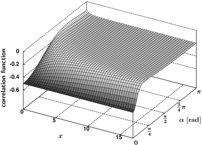
Figure 1: The plot shows the dependence of the correlation function $\mathcal{C}^{\xi(k,p_{k})}_{\textsf{polarization}}(k,\theta;p_{k},\tilde{\theta})$ [Eq. (81)] on $x$ and $\alpha$ for $\theta=5\pi/6$, $\tilde{\theta}=8.69\pi/6$.

Figure 2: The plot shows the dependence of the correlation function $\mathcal{C}^{\xi(k,p_{k})}_{\textsf{polarization}}(k,\theta;p_{k},\tilde{\theta})$ [Eq. (81)] on $x$ for k orthogonal to p ($\alpha=\pi/2$), and $\theta=5\pi/6$, $\tilde{\theta}=8.69\pi/6$.

VI.1 Bell-type inequalities

In this subsection we will show that the degree of violation of Bell-type inequalities strongly depends on the particle momenta. In the local realistic theory the CHSH inequality Clauser et al. (1969); Ballentine (1998)

$$|\mathcal{C}_{ab}-\mathcal{C}_{ad}|+|\mathcal{C}_{cb}+\mathcal{C}_{cd}|\leq 2$$ (82)

should hold. In Eq. (82) $\mathcal{C}_{ab}$ denotes the correlation function of observables with eigenvalues $1$, $0$, and $-1$, parametrized by $a$ and $b$, and measured by Alice and Bob. Therefore, the CHSH inequality (82) in the local realistic theory should be satisfied also for the polarization correlation function (68). Let us consider the CHSH inequality (82) for the polarization correlation function in the state $|\xi(k,k^{\pi})\rangle$ in the center of mass frame

$$\big{|}\mathcal{C}^{\xi(k,k^{\pi})}_{\textsf{polarization}}(k,\theta_{a};k^{\pi},\theta_{b})-\mathcal{C}^{\xi(k,k^{\pi})}_{\textsf{polarization}}(k,\theta_{a};k^{\pi},\theta_{d})\big{|}\\ +\big{|}\mathcal{C}^{\xi(k,k^{\pi})}_{\textsf{polarization}}(k,\theta_{c};k^{\pi},\theta_{b})+\mathcal{C}^{\xi(k,k^{\pi})}_{\textsf{polarization}}(k,\theta_{c};k^{\pi},\theta_{d})\big{|}\leq 2$$ (83)

Inserting Eq. (80) into Eq. (83) we get

$$\frac{2(2x+1)^{2}}{2(2x+1)^{2}+1}\Big{\{}\big{|}\cos 2(\theta_{a}+\theta_{b})-\cos 2(\theta_{a}+\theta_{d})\big{|}\\ +\big{|}\cos 2(\theta_{c}+\theta_{b})+\cos 2(\theta_{c}+\theta_{d})\big{|}\Big{\}}\leq 2$$ (84)

The left side of Eq. (84) is largest in the configuration in which $\big{|}\cos 2(\theta_{a}+\theta_{b})-\cos 2(\theta_{a}+\theta_{d})\big{|}+\big{|}\cos 2(\theta_{c}+\theta_{b})+\cos 2(\theta_{c}+\theta_{d})\big{|}$ has maximum value. But the analysis of the standard nonrelativistic CHSH inequality shows that the maksimum value of this quantity is equal to $2\sqrt{2}$ (we receive this value for e.g. $\theta_{a}=0$, $\theta_{b}=\pi/8$, $\theta_{c}=6\pi/8$, and $\theta_{d}=3\pi/8$). The dependence of the left side of inequality (84) in the above configuration is shown in Fig. 3.

Figure 3: The plot shows the dependence of the left side of the inequality (84) for $\theta_{a}=0$, $\theta_{b}=\pi/8$, $\theta_{c}=6\pi/8$, and $\theta_{d}=3\pi/8$ on $x$. The inequality (84) is violated for $x>x_{0}=-\frac{1}{2}+\frac{1}{2\sqrt{2\sqrt{2}-2}}\approx 0.049$.

One can see that the degree of violation of this inequality strongly depends on the particle momentum. Moreover, the left side of the inequality (84) increases with the particle momentum and reaches the limiting value $2\sqrt{2}$ in the ultrarelativistic (massless) limit. It should be also noted that in the nonrelativistic case ($x=0$) the inequality (84) is not violated (the left side of the inequality (84) is equal to $\frac{4\sqrt{2}}{3}$).

VII Conclusions

We have calculated the helicity and linear polarization correlation functions of two relativistic vector bosons in certain scalar states. To discuss linear polarization correlations we have defined states corresponding to the longitudal and transversal polarization of vector particle. In particular we have found the scalar state which in the massless limit tends to the two-photon scalar state. We have shown also that in the massless limit the polarization correlation function in this scalar state tends to the correlation function in the scalar two-photon state. We have considered also the CHSH inequality and found that the degree of violation of this inequality can increase with the particle momentum. Such a behaviour can be important in applications of relativistic massive particles in various quantum information protocols, like e.g. quantum cryptography based on violation of Bell inequalities Ekert (1991).