Scaling behavior of self-avoiding walks on percolation clusters

Abstract

The scaling behavior of self-avoiding walks (SAWs) on the backbone of percolation clusters in two, three and four dimensions is studied by Monte Carlo simulations. We apply the pruned-enriched Rosenbluth chain-growth method (PERM). Our numerical results bring about the estimates of critical exponents, governing the scaling laws of disorder averages of the end-to-end distance of SAW configurations. The effects of finite-size scaling are discussed as well.

1 Introduction

The universal configurational properties of long, flexible polymer chains in a good solvent are perfectly described by the model of self-avoiding walks (SAWs) on a regular lattice [1]. In particular, the average square end-to-end distance $\langle R^{2}\rangle$, and the number of configurations $Z_{N}$ of SAWs with $N$ steps obey the scaling laws:

$$\langle R^{2}\rangle\sim N^{2\nu_{\rm SAW}},\mbox{\hskip 30.00005pt}Z_{N}\sim z^{N}N^{\gamma_{\rm SAW}-1},$$ (1)

where $\nu_{{\rm SAW}}$ and $\gamma_{{\rm SAW}}$ are the universal critical exponents that only depend on the space dimension $d$, and $z$ is a non-universal connectivity constant, depending also on the type of the lattice. The properties of SAWs on a regular lattice have been studied in detail both in computer simulations [2, 3, 4, 5, 6, 7] and analytical approaches [8, 9, 10, 11]. For example, in the space dimension $d{=}3$ one finds within the frame of the field-theoretical renormalization group approach $\nu_{\rm SAW}{=}0.5882\pm 0.0011$ [11] and Monte Carlo simulations give $\nu_{\rm SAW}{=}0.5877\pm 0.0006$ [5]. For space dimensions $d$ above the upper critical dimension $d_{\rm up}{=}4$, the scaling exponent becomes trivial: $\nu_{\rm SAW}(d\geq 4){=}1/2$.

A question of great interest is how SAWs behave on randomly diluted lattices, which may serve as a model of linear polymers in a porous medium. Numerous numerical [12, 13, 14, 15, 16, 17, 18, 19, 20, 21, 22] and analytical [17, 23, 24, 25, 26, 27, 28, 29] studies lead to the conclusion that weak quenched disorder, when the concentration $p$ of lattice sites allowed for the SAWs is higher than the percolation concentration $p_{c}$, does not influence the scaling of SAWs. The scaling laws (1) are valid in this case with the same exponents, independently of $p$. More interesting is the case, when $p$ equals the critical concentration $p_{c}$ (see Table 1) and the lattice becomes percolative. Studying properties of percolative lattices, one encounters two possible statistical averages. In the first, one considers only incipient percolation clusters whereas the other statistical ensemble includes all the clusters, which can be found in a percolative lattice. For the latter ensemble of all clusters, the SAW can start on any of the clusters, and for an $N$-step SAW, performed on the $i$th cluster, we have $\langle R^{2}\rangle\sim l_{i}^{2}$, where $l_{i}$ is the averaged size of the $i$th cluster. In what follows, we will be interested in the former case, when SAWs reside only on the percolation cluster. In this regime, the scaling laws (1) hold with new exponents $\nu_{p_{c}}\neq\nu_{{\rm SAW}},\gamma_{p_{c}}\neq\gamma_{{\rm SAW}}$ [14, 15, 16, 20, 21, 30, 31]. A hint to the physical understanding of this phenomenon is given by the fact that weak disorder does not change the dimension of a lattice, whereas the percolation cluster itself is a fractal with fractal dimension $d_{p_{c}}^{F}$ dependent on $d$ (see Table 1). In this way, scaling law exponents of SAWs change with the dimension $d_{p_{c}}^{F}$ of the (fractal) lattice on which the walk resides. Since $d_{\rm up}{=}6$ for percolation [39], the exponent $\nu_{p_{c}}(d\geq 6){=}1/2$. For the connectivity constant $z_{p_{c}}$ of SAWs on a percolative lattice the estimate $z_{p_{c}}{=}p_{c}z$ is suggested, where $z$ is the value on the corresponding pure lattice [32].

Table 1: Critical concentration $p_{c}$ of site-diluted lattices and fractal dimensions of percolation cluster $d_{p_{c}}^{F}$ and backbone of the percolation cluster $d_{p_{c}}^{B}$ for different space dimensions $d$.

$d$	$p_{c}$	$d_{p_{c}}^{F}$	$d_{p_{c}}^{B}$
2	$0.592746$ [33]	$91/49$ [36]	$1.650\pm 0.005$ [38]
3	$0.31160$ [34]	$2.51\pm 0.02$ [37]	$1.86\pm 0.01$ [38]
4	$0.19688$ [35]	$3.05\pm 0.05$[37]	$1.95\pm 0.05$[38]

Until recently there did not exist any satisfactory theoretical estimates for scaling law exponents of SAWs on percolation clusters, based on refined field-theoretical approaches. In particular this was caused by the rather complicated diagrammatic technique of the perturbation theory calculations. Recently the field theory developed by Meir and Harris [17] was reconsidered in Refs. [30, 31], where the field theory with complex interacting fields has been constructed and a special diagrammatic technique developed. The scaling properties of a SAW on a percolation cluster were found to be described by a whole family of correlation exponents $\nu^{(i)}$, with $\nu^{(1)}{=}\nu_{\rm SAW}$.

Note that up to date there do also not exist many studies dedicated to Monte Carlo (MC) simulations of our problem and they do still exhibit some controversies. The first MC study of a SAW statistics on a disordered (diluted) lattice in three dimensions was performed in the work of Kremer [12]. It indicates no change in the exponent $\nu$ for weak dilution, but for concentrations of dilution near the percolation threshold a higher value $\nu_{{p_{c}}}\approx 2/3$ was observed.

This result was the only numerical estimate of $\nu_{p_{c}}$ for a number of years, until Lee et al. [13, 14] performed MC simulations for a SAW on the percolation cluster for square and cubic lattices at dilutions very close to the percolation threshold. Two earlier of these works indicate the rather surprising result that in two dimensions the critical exponent $\nu_{{p_{c}}}$ is not different compared to the pure lattice value. Later, some numerical uncertainties were corrected and the value for $\nu_{{p_{c}}}$ found in two dimensions is in a new universality class. This result has been confirmed in a more accurate study of Grassberger [15]. In the case of three and four dimensions, there also exist estimates indicating a new universality class [14], but no satisfactory numerical values have been obtained so far. It was argued in Ref. [20], that series enumerations of all possible SAW configurations on a percolation cluster give a greater value for $\nu_{p_{c}}$ (and therefore in better agreement with theoretical prediction) than that obtained from MC simulations due to some specific peculiarities of the latter method.

In the present paper, the so-called chain-growth algorithm is applied. Conventional MC methods such as multicanonical sampling [40] or the Wang-Landau method [41] expose problems in tackling “hidden” conformational barriers in combination with chain update moves which usually become inefficient at low temperatures, where many attempted moves are rejected due to the self-avoidance constraint. Rosenbluth chain growth avoids occupied neighbors at the expense of a bias. Chain-growth methods with population control such as PERM (pruned-enriched Rosenbluth method) [42, 43] improve the procedure considerably by utilizing the counterbalance between Rosenbluth weight and Boltzmann probability. PERM has been applied successfully to a wide class of problems, in particular to the $\Theta$-transition of homopolymers [42], trapping of random walkers on absorbing lattices[44], study of protein folding [45], etc.

2 Construction of percolation clusters

We consider site percolation on regular lattices of edge lengths up to $L_{{\rm max}}{=}300,200,50$ in dimensions $d{=}2,3,4$, respectively. Each site of the lattice was assigned to be occupied with probability $p_{c}$ (values of critical concentration in different dimensions are given in Table 1), and empty otherwise. To extract the percolation cluster, we apply the algorithm of site labeling, based on the one proposed by Hoshen and Kopelman [46]. If for a given lattice it is not possible to find a cluster that wraps around in all coordinate directions, this disordered lattice is rejected and a new one is constructed. The typical structure of percolation clusters is presented in Fig. 1. On finite lattices the definition of spanning clusters is not unique (e.g., one could consider clusters connecting only two opposite borders), but all definitions are characterized by the same fractal dimension and are thus equally legitimate. The here employed definition has the advantage of yielding the most isotropic clusters. Note also that directly at $p=p_{c}$ more than one spanning cluster can be found in the system, and the probability $P(k)$ for at least $k$ separated clusters grows with the space dimension as $P(k)\sim\exp(-\alpha k^{d/(d-1)})$ [47, 48]. In our study, we take into account only one cluster per each disordered lattice constructed, in order to avoid presumable correlations of the data.

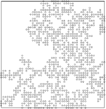
Figure 1: Percolation cluster on a $d{=}2$-dimensional regular lattice of edge length $L{=}50$.

Since we aim on investigating the scaling of SAWs on a percolative lattice, we are interested rather in the backbone of the percolation cluster, which is defined as follows. Assume that each bond (or site) of the cluster is a resistor and that an external potential drop is applied at two ends of the cluster. The backbone is the subset of the cluster consisting of all bonds (or sites) through which the current flows; i.e., it is the structure left when all “dangling ends” are eliminated from the cluster. The SAWs can be trapped in “dangling ends”, therefore infinitely long chains can only exist on the backbone of the cluster.

The algorithm for extracting the backbone of a given percolation cluster was first introduced in [49] and improved in [50]. This so-called burning algorithm is divided into two parts. First, we choose the starting point –“seed” – at the center of the cluster. For all the sites on the edge of the lattice, belonging to the percolation cluster, we find the shortest paths between the “seed” and the given site. As a result, we obtain a so-called skeleton or elastic backbone [51] of the percolation cluster, shown in Fig. 2, left.

In the second part of the algorithm, we consider successively each site of the elastic backbone and check whether a “loop” starts from this site. A “loop” is a path of sites, belonging to the percolation cluster, which is connected with the elastic backbone by no less than two sites. Sites of the elastic backbone together with sites of “loops” form finally the geometric backbone of the cluster (see Fig. 2, right).

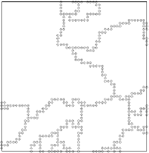
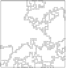
Figure 2: Elastic (left) and geometrical (right) backbones of the percolation cluster depicted in Fig. 1.

Once a cluster is generated, its fractal dimension in topological (or chemical) space $l$ can be determined according to [50]:

$$\langle M_{B}({l})\rangle\sim{l}^{d_{B}^{{l}}},$$ (2)

where $M_{B}(l)$ is its “mass” (number of cluster sites) and $d_{B}^{{l}}$ is the fractal dimension of the backbone in chemical space. It is related to the dimension $d_{p_{c}}^{B}$ in coordinate space by $d_{p_{c}}^{B}{=}d_{B}^{{l}}d_{{\rm min}}$, where $d_{{\rm min}}$ is the fractal dimension of the shortest path on the backbone and describes the scaling behavior between $r$ and ${l}$, i.e. $\langle{l}\rangle\sim r^{d_{{\rm min}}}$, with $d_{{\rm min}}{=}1.130\pm 0.004$ in $d{=}2$ [52], $d_{{\rm min}}{=}1.374\pm 0.003$ in $d{=}3$ [34], $d_{{\rm min}}{=}1.567$ in $d{=}4$ [53]. The results for fractal dimensions of the percolation cluster and its geometrical backbone in $d{=}2,3,4$ are compiled in Table 1.

3 The method

We use the pruned-enriched Rosenbluth method (PERM), proposed in the work of Grassberger [42]. The algorithm is based on ideas from the very first days of Monte Carlo simulations, the Rosenbluth-Rosenbluth (RR) method [2] and enrichment strategies [54]. Let us consider the growing polymer chain, i.e., the $n$th monomer is placed at a randomly chosen neighbor site of the last placed $(n-1)$th monomer ($n\leq N$, where $N$ is the total length of the chain). In order to obtain correct statistics, if this new site is occupied, any attempt to place a monomer at it results in discarding the entire chain. This leads to an exponential “attrition”, the number of discarded chains grows exponentially with the chain length, which makes the method useless for long chains. In the RR method, occupied neighbors are avoided without discarding the chain, but the bias is corrected by means of giving a weight $W_{n}\sim(\prod_{l{=}2}^{n}m_{l})^{-1}$ to each sample configuration at the $n$th step, where $m_{l}$ is the number of free lattice sites to place the $l$th monomer. When the chain of total length $N$ is constructed, the new one starts from the same starting point, until the desired number of chain configurations are obtained. The configurational averaging for the end-to-end distance $r\equiv\sqrt{R^{2}(N)}$ is then given by:

$$\langle{r}\rangle{=}\frac{\sum_{{\rm conf}}W_{N}^{{\rm conf}}r^{{\rm conf}}}{\sum_{{\rm conf}}W_{N}^{{\rm conf}}}{=}\sum_{r}rP(r,N),$$ (3)

where $W_{N}^{{\rm conf}}$ is the weight of an $N$-monomer chain in a given configuration and $P(r,N)$ is the distribution function for the end-to-end distance.

\psfrag{xx}{$r/N^{\nu_{p_{c}}}$}\psfrag{yy}{$r\overline{P(r,N)}$}\includegraphics[width=150.79968pt]{rozpR3d.eps}

Figure 3: Disorder averaged distribution function $r\overline{P(r,N)}$ vs the scaling variable $r/N^{\nu_{p_{c}}}$ in $d{{=}}3$ dimensions. Lattice size $L{{=}}200$, number of SAW steps $N{{=}}40$ (squares), $N{{=}}50$ (pluses), $N{{=}}60$ (diamonds), $N{{=}}70$ (crosses), $N{{=}}80$ (stars).

\psfrag{xx}{$r/N^{\nu_{p_{c}}}$}\psfrag{yy}{$r\overline{P(r,N)}$}\includegraphics[width=150.79968pt]{rozpR4d.eps}

Figure 4: Disorder averaged distribution function $r\overline{P(r,N)}$ vs the scaling variable $r/N^{\nu_{p_{c}}}$ in $d{{=}}4$ dimensions. Lattice size $L{{=}}50$, number of SAW steps $N{{=}}15$ (squares), $N{{=}}18$ (triangles), $N{{=}}20$ (pluses), $N{{=}}25$ (crosses), $N=30$ (stars).

While the chain grows by adding monomers, its weight will fluctuate. PERM suppresses these fluctuations by pruning configurations with too small weights, and by enriching the sample with copies of high-weight configurations [42]. These copies are made while the chain is growing, and continue to grow independently of each other. Pruning and enrichment are performed by choosing thresholds $W_{n}^{<}$ and $W_{n}^{>}$ depending on the estimate of the partition sums of the $n$-monomer chain. These thresholds are continuously updated as the simulation progresses. The zeroes iteration is a pure chain-growth algorithm without reweighting. After the first chain of full length has been obtained, we switch to $W_{n}^{<}$, $W_{n}^{>}$. If the current weight $W_{n}$ of an $n$-monomer chain is less than $W_{n}^{<}$, a random number $r{=}{0,1}$ is chosen; if $r{=}0$, the chain is discarded, otherwise it is kept and its weight is doubled. Thus, low-weight chains are pruned with probability $1/2$. If $W_{n}$ exceeds $W_{n}^{>}$, the configuration is doubled and the weight of each copy is taken as half the original weight. For updating the threshold values we apply similar rules as in [43, 45]: $W_{n}^{>}{=}C(Z_{n}/Z_{1})(c_{n}/c_{1})^{2}$ and $W_{n}^{<}{=}0.2W_{n}^{>}$, where $c_{n}$ denotes the number of created chains having length $n$, and the parameter $C$ controls the pruning-enrichment statistics. After a certain number of chains of total length $N$ is produced, the iteration is finished and a new tour starts. We adjust the pruning-enrichment control parameter such that on average 10 chains of total length $N$ are generated per each iteration [45], and perform $10^{6}$ iterations. Also, what is even more important for efficiency, in almost all iterations at least one such a chain was created.

\psfrag{xx}{$\ln N$}\psfrag{yy}{$\ln{\overline{\langle r\rangle}}$}\includegraphics[width=170.71652pt]{sawr.eps}

Figure 5: Disorder averaged end-to-end distance vs number of steps in double logarithmic scale for SAWs on the backbone of percolation clusters in $d{=}2$ (pluses), $d{=}3$ (stars), $d{=}4$ (squares). Lines represent linear fitting, statistical error bars are of the size of symbols.

4 Results

To study scaling properties of SAWs on the backbone of percolation clusters, we choose as the starting point the “seed” of the cluster, and apply the PERM algorithm, taking into account, that a SAW can have its steps only on the sites belonging to the backbone of the percolation cluster. In the given problem, we have to perform two types of averaging: the first average is performed over all SAW configurations on a single backbone according to (3); the second average is carried out over different realizations of disorder, i.e. over many backbone configurations:

$$\overline{\langle r\rangle}{=}\frac{1}{C}\sum_{c{=}1}^{C}\langle r\rangle_{c}{=}\sum_{r}r{\overline{P(r,N)}},$$ (4)

$$\overline{P(r,N)}{=}\frac{1}{C}\sum_{c{=}1}^{C}P_{c}(r,N).$$ (5)

Here, $C$ is the number of different clusters, the index $c$ means that a given quantity is calculated on the cluster $c$, $\overline{P(r,N)}$ is the distribution function, averaged over cluster configurations.

Table 2: Results of linear fitting of obtained results for $\overline{\langle r\rangle}$ for SAWs in $d{=}3$ dimensions on the backbone of percolation clusters, $L{=}200$. $\chi^{2}$ denotes the sum of squares of normalized deviation from the regression line, $DF$ is the number of degrees of freedom.

$N_{{\rm min}}$	$\nu_{p_{c}}$	$a$	$\chi^{2}/DF$
6	0.665 $\pm$ 0.003	0.946 $\pm$ 0.003	2.783
11	0.668 $\pm$ 0.003	0.935 $\pm$ 0.004	2.269
16	0.669 $\pm$ 0.003	0.930 $\pm$ 0.004	2.054
21	0.669 $\pm$ 0.003	0.924 $\pm$ 0.004	1.345
26	0.667 $\pm$ 0.002	0.930 $\pm$ 0.006	0.743
31	0.668 $\pm$ 0.002	0.934 $\pm$ 0.008	0.844

The case of so-called “quenched disorder” is considered, where the average over different realizations of disorder is taken after the configurational average has been performed. As it was pointed out in [15], the correctness of results, obtained in the picture of “quenched” disorder, depends on whether the location of the starting point of a SAW is fixed while the configurational averaging is performed, or not. In the latter case, one has to average over all locations and effectively this corresponds to the case of annealed disorder. Thus, as we have already stated above, we start each configuration of a SAW on the same site – the “seed” of the backbone of a given percolation cluster. We use lattices of the size up to $L_{{\rm max}}{=}300,200,50$ in $d{=}2,3,4$, respectively, and performed averages over 1000 percolation clusters in each case.

The disorder averaged distribution function (5) can be written in terms of the scaled variables $r/\overline{\langle r\rangle}$ as:

$$r\overline{P(r,N)}\sim f(r/\overline{\langle r\rangle})\sim f(r/N^{\nu_{p_{c}}}).$$ (6)

The distribution function is normalized according to $\sum_{r}{\overline{P(r,N)}}{{=}}1$. The numerical results for the distribution function in $d{{=}}3$ and $d{{=}}4$ are shown in Figs. 3 and 4 for different $N$. When plotted against the scaling variable $r/N^{\nu_{p_{c}}}$, the data are indeed found to nicely collapse onto a single curve, using our values for the exponent $\nu_{p_{c}}$ reported in Table 3 below.

To estimate the critical exponents $\nu_{p_{c}}$, linear least-square fits with lower cutoff for the number of steps $N_{{\rm min}}$ are used. The $\chi^{2}$ value (sum of squares of normalized deviation from the regression line) serves as a test of the goodness of fit (see Fig. 5 and Table 2).

Since we can construct lattices only of a finite size $L$, it is not possible to perform very long SAWs on it. For each $L$, the scaling (1) holds only up to some “marginal” number of SAWs steps $N_{{\rm marg}}$, as it is shown in Fig. 6. We take this into account when analyzing the data obtained; for each lattice size we are interested only in values of $N<N_{{\rm marg}}$, which results in effects of finite-size scaling for critical exponents.

\psfrag{xx}{$\ln N$}\psfrag{yy}{$\ln\langle r\rangle$}\includegraphics[width=113.81102pt]{finit2d.eps}

\psfrag{xx}{$\ln N$}\psfrag{yy}{$\ln\langle r\rangle$}\psfrag{xx}{$\ln N$}\psfrag{yy}{$\ln{\overline{\langle r\rangle}}$}\includegraphics[width=113.81102pt]{finit2p.eps}

Figure 6: Averaged end-to-end distance vs number of steps on a double logarithmic scale for SAWs on a pure lattice (left) and on the backbone of a percolation cluster (right) in $d{{=}}2$. In both cases the lattice size $L$ changes from below: $L{{=}}50,80,100,150,200$. Error bars are of the size of symbols.

\psfrag{xx}{$N/L^{\omega}$}\psfrag{yy}{$g(N/L^{\omega})$}\includegraphics[width=113.81102pt]{scal2pure.eps}

\psfrag{xx}{$N/L^{\omega}$}\psfrag{yy}{$g(N/L^{\omega})$}\psfrag{xx}{$N/L^{\omega}$}\psfrag{yy}{$g(N/L^{\omega})$}\includegraphics[width=113.81102pt]{scal2pc.eps}

Figure 7: The scaling function $g(N/L^{\omega})$ as a function of its argument at data collapse for three different lattice sizes $L{{=}}100,150,200$ in $d{{=}}2$. Left: pure lattice, right: backbone of the percolation cluster.

Let us assume that $N_{{\rm marg}}\sim L^{\omega}$, and for a SAW confined inside a lattice with size $L$ finite-size scaling holds:

$$\langle r\rangle\sim N^{\nu}g(\frac{N}{L^{\omega}}),$$ (7)

where

$$g(x){=}{\rm const}{\mbox{\,}\,\,{\rm when}\,\,\,}N\ll L^{\omega}$$

so that Eq. (1) is recovered. The crossover occurs at ${\langle r\rangle}\sim L,N{=}N_{{\rm marg}}$, which leads to $\omega{=}1/\nu$. Here, $\nu$ stands for $\nu_{{\rm SAW}}$ or $\nu_{p_{c}}$ for the cases of the pure lattice and backbone of percolation cluster, respectively. Similar scaling properties have already been observed in problems of random walks in confined environment in Ref. [55].

Table 3: The exponent $\nu_{p_{c}}$ for a SAW on a percolation cluster. FL: Flory-like theories, EE: exact enumerations, RS, RG: real-space and field-theoretic RG. For SAWs on the regular lattice one has: $\nu_{{\rm SAW}}(d{{=}}2){=}3/4$ [9], $\nu_{{\rm SAW}}(d{{=}}3){=}0.5882(11)$ [11], $\nu_{{\rm SAW}}(d\geq 4){=}1/2$.

$\nu_{p_{c}}\setminus d$	2	3	4
FL [28]	0.77	0.66	0.62
EE [20]	0.770(5)	0.660(5)
[21]	0.778(15)	0.66(1)
[21]	0.787(10)	0.662(6)
RS [29]	0.767
[25]	0.778	0.724
RG [30]	0.785	0.678	0.595
[31]	0.796	0.669	0.587
MC [14]	0.77(1)
[15]	0.783(3)
[16]		0.62–0.63	0.56–0.57
our results	$0.782\pm 0.003$	$0.667\pm 0.003$	$0.586\pm 0.003$

Having estimated values for the critical exponent $\nu_{p_{c}}$, presented in Table 3, we can proceed with testing the finite-size scaling assumption (7). When plotted against the scaling variable $N/L^{\omega}$, the data for different lattice sizes $L$ should collapse onto a single curve if we have found the correct values for the critical exponents. The numerical results for the scaling function $g(N/L^{\omega})$ both for the pure lattice (for comparison) and the backbone of percolation clusters are presented in Fig. 7. Note, that our estimation of the exponent $\nu_{{\rm SAW}}$ in two dimensions gives $0.745\pm 0.002$.

5 Conclusions

The present paper concerns the universal configurational properties of SAWs on percolative lattices. The statistical averaging was performed on the backbone of the incipient percolation cluster, which has a fractal structure and is characterised by fractal dimension $d_{p_{c}}^{B}$. Note, that up to date there do not exist many works dedicated to Monte Carlo (MC) simulations of our problem and they do still exhibit some controversies. In particular, in the case of four dimensions, there exist only estimates, indicating a new universality class [14], but no satisfactory numerical values for critical exponents have been obtained so far.

Applying the pruned-enriched Rosenbluth method (PERM), we studied SAWs on the backbone of percolation clusters, using lattices of size up to $L_{{\rm max}}{=}300,200,50$ in $d{=}2,3,4$, respectively, and performing averages over 1000 clusters in each case. Our results bring about numerical values of critical exponents, governing the end-to-end distance of SAWs in a new universality class. The effects of finite lattice size are discussed as well.

- [1] \Namedes Cloizeaux J. Jannink G. \BookPolymers in Solution \PublClarendon Press, Oxford \Year1990; \Namede Gennes P.-G. \Book Scaling Concepts in Polymer Physics \PublCornell University Press, Ithaca and London \Year1979.
- [2] \NameRosenbluth M.N. Rosenbluth A.W. \REVIEWJ. Chem. Phys.231955356.
- [3] \NameMadras N. Sokal A.D. \REVIEWJ. Stat. Phys.501988109.
- [4] \NameMac Donald D., Hunter D.L., Kelly K. Naeem J. \REVIEWJ. Phys. A2519921429.
- [5] \NameLi B., Madras N. Sokal A.D. \REVIEWJ. Stat. Phys. 801995661.
- [6] \NameCaracciolo S., Causo M.S. Pelissetto A. \REVIEWPhys. Rev. E 571998 R1215.
- [7] \NameMacDonald D., Joseph S., Hunter D.L., Moseley L.L., Jan N. Guttmann A.J. \REVIEWJ. Phys. A3320005973.
- [8] \NameLe Guillou J.C. Zinn-Justin J. \REVIEWPhys. Rev. B 21 1980 3976.
- [9] \NameNienhuis B. \REVIEWPhys. Rev. Lett. 491982 1062.
- [10] \NameLe Guillou J.C. Zinn-Justin J. \REVIEWJ. Physique Lett. 461985 L127; \REVIEWJ. Physique 50 1988 1365.
- [11] \NameGuida R. Zinn Justin J. \REVIEW J. Phys. A 311998 8104.
- [12] \NameKremer K. \REVIEWZ. Phys. B 451981 149.
- [13] \NameLee S.B. Nakanishi H. \REVIEWPhys. Rev. Lett. 6119882022; \NameLee S.B., Nakanishi H. Kim Y. \REVIEWPhys. Rev. B 3919899561.
- [14] \NameWoo K.Y. Lee S.B. \REVIEWPhys. Rev. A 441991999.
- [15] \NameGrassberger P. \REVIEWJ. Phys. A 2619931023.
- [16] \NameLee S.B.\REVIEW J. Korean Phys. Soc. 2919961.
- [17] \NameMeir Y. Harris A.B.\REVIEW Phys. Rev. Lett. 6319892819.
- [18] \NameLam P.M. \REVIEWJ. Phys. A 231990L831.
- [19] \NameNakanishi H. Moon J. \REVIEW Physica A 1911992309.
- [20] \NameRintoul M.D., Moon J. Nakanishi H. \REVIEW Phys. Rev. E 491994 2790.
- [21] \NameOrdemann A., Porto M., Roman H.E., Havlin S. Bunde A. \REVIEWPhys. Rev. E6120006858.
- [22] \NameNakanishi H. Lee S.B. \REVIEW J. Phys. A 2419911355.
- [23] \NameKim Y.\REVIEW J. Phys. C 1619831345.
- [24] \NameBarat K., Karmakar S.N. Chakrabarti B.K. \REVIEWJ. Phys. A241991851.
- [25] \NameSahimi M. \REVIEW J. Phys. A 171984L379.
- [26] \Name Rammal R., Toulouse G. Vannimenus J. \REVIEWJ. Phys. (Paris) 45 1984 389.
- [27] \NameKim Y. \REVIEW J. Phys. A 2019871293.
- [28] \NameRoy A.K. Blumen A. \REVIEWJ. Stat. Phys. 5919901581.
- [29] \NameLam P.M. Zhang Z.Q. \REVIEW Z. Phys. B 561984155.
- [30] \Namevon Ferber C., Blavatska V., Folk R. Holovatch Yu. \REVIEW Phys. Rev. E 702004035104(R).
- [31] \NameJanssen H.-K. Stenull O. \REVIEWPhys. Rev. E 752007 020801(R).
- [32] \NameChakrabarti B.K., Bhadra K., Roy A.K. Karmakar S. N. \REVIEWPhys. Lett. A931983434.
- [33] \NameZiff R.M. \REVIEWPhys. Rev. Lett. 7219941942.
- [34] \NameGrassberger P. \REVIEWJ. Phys. A 251992 5867.
- [35] \NamePaul G., Ziff R.M. Stanley H.E. \REVIEWPhys. Rev. E 642001026115.
- [36] \NameHavlin S. Ben Abraham D. \REVIEWAdv. Phys. 361987155.
- [37] \NameGrassberger P. \REVIEW J. Phys. A 1919861681.
- [38] \NameMoukarzel C. \REVIEWInt. Journal of Mod. Phys. C81998887.
- [39] \NameStauffer D. Aharony A. \BookIntroduction to Percolation Theory \PublTaylor and Francis, London \Year1992.
- [40] \NameBerg B.A. Neuhaus T. \REVIEW Phys. Lett. B 267 1991249.
- [41] \NameWang F. Landau D.P. \REVIEWPhys. Rev. Lett. 8620012050.
- [42] \NameGrassberger P. \REVIEW Phys. Rev. E 561997 3682.
- [43] \NameHsu H.P., Mehra V., Nadler W. Grassberger P. \REVIEW J. Chem. Phys. 1182007444.
- [44] \NameMehra V. Grassberger P. \REVIEW Physica D1682002244.
- [45] \NameBachmann M. Janke W. \REVIEW Phys. Rev. Lett. 912003208105; \REVIEWJ. Chem. Phys.12020046779.
- [46] \NameHoshen J. Kopelman R. \REVIEW Phys. Rev. E 14 1976 3438.
- [47] \Name Aizenman M. \REVIEW Nucl. Phys. B [FS] 485 1997 551.
- [48] \Name Shchur L.N. Rostunov T. \REVIEW JETP Lett. 762002 475.
- [49] \Name Herrmann H.J., Hong D.C. Stanley H.E. \REVIEW J. Phys. A 171984 L261.
- [50] \NamePorto M., Bunde A., Havlin S. Roman H.E. \REVIEW Phys. Rev. E 5619971667.
- [51] \NameHavlin S., Nossal R., Trus B. Weiss G.H. \REVIEW J. Phys. A 17 1984L957.
- [52] \Name Herrmann H.J. Stanley H.E. \REVIEW J. Phys. A 211988 L829.
- [53] \NameJanssen H.-K. Stenull O. \REVIEWPhys. Rev. E61 20004821.
- [54] \Name Wall F.T. Erpenbeck J.J. \REVIEWJ. Chem. Phys.30 1959 634.
- [55] \NameReis F. \REVIEW J. Phys. A 281995 6277.