Monte Carlo simulations of the directional-ordering transition in the two-dimensional classical and quantum compass model

Abstract

A comprehensive study of the two-dimensional (2D) compass model on the square lattice is performed for classical and quantum spin degrees of freedom using Monte Carlo and quantum Monte Carlo methods. We employ state-of-the-art implementations using Metropolis, stochastic series expansion and parallel tempering techniques to obtain the critical ordering temperatures and critical exponents. In a pre-investigation we reconsider the classical compass model where we study and contrast the finite-size scaling behavior of ordinary periodic boundary conditions against annealed boundary conditions. It is shown that periodic boundary conditions suffer from extreme finite-size effects which might be caused by closed loop excitations on the torus. These excitations also appear to have severe effects on the Binder parameter. On this footing we report on a systematic Monte Carlo study of the quantum compass model. Our numerical results are at odds with recent literature on the subject which we trace back to neglecting the strong finite-size effects on periodic lattices. The critical temperatures are obtained as $T_{\mathrm{c}}=0.1464(2)J$ and $T_{\mathrm{c}}=0.055(1)J$ for the classical and quantum versions, respectively, and our data support a transition in the 2D Ising universality class for both cases.

I Introduction

The compass model is one of the simplest models possessing orbital degenerate states. Originally developedKugel and Khomskii (1982) as a model for Mott insulators it has recently seen renewed interestNussinov et al. (2004); Khomskii and Mostovoy (2003); Mostovoy and Khomskii (2004) in connection with orbital-order in materials like transition metal (TM) compounds. Despite its closeness to ordinary models of quantum magnetism, like the Heisenberg model, there is no ordered phase characterized by magnetization properties. This means that the ordered phase appearing in the model is especially interesting in that it cannot be classified according to the Mermin-Wagner criterion. A competition of interactions in different directions rather results in a special long-range ordered stateMishra et al. (2004) possessing a sense of orientation, and the transition is at the same time accompanied by dimensional reduction.Batista and Nussinov (2005) The current interest in this model is furthermore triggered by the recent discovery that it describes arrays of superconducting Josephson junctions and because of a possible realization of a system which protects qubits against unwanted decay in quantum computation.Douçot et al. (2005); Milman et al. (2007)

The compass model is a spin model on simple-cubic lattices in $d$ dimensions of size $N=L^{d}$ defined by the Hamiltonian

$$\mathcal{H}=\sum_{i}\sum^{d}_{k}J_{k}S^{k}_{i}S^{k}_{i+e_{k}}\,,$$ (1)

where $S^{k}_{i}$ represents the $k$-th component of a spin $\mathbf{S}$ at site $i$ and $i+e_{k}$ is the nearest neighbor of $i$ in the $k$ direction. In the classical case we have $\mathbf{S}\in O(d)$, or in a more explicit vector representation with $\varphi$ and $\theta$ being angles on the sphere, we use the expression $\mathbf{S}^{\mathsf{T}}=\left(\cos(\varphi),\sin(\varphi)\right)$ and $\mathbf{S}^{\mathsf{T}}=\left(\cos(\varphi)\sin(\theta),\sin(\varphi)\sin(\theta),\cos(\theta)\right)$ in two and three dimensions, respectively. In the two-dimensional (2D) quantum case $\mathbf{S}$ represents a spin-$1/2$ operator $\mathbf{S}=(1/2)\,(\sigma_{x},\sigma_{z})$ and the Hamiltonian assumes the form

$$\mathcal{H}=(1/4)\,\sum_{i}\left(J_{x}\sigma^{x}_{i}\sigma^{x}_{i+e_{x}}+J_{z}\sigma^{z}_{i}\sigma^{z}_{i+e_{z}}\right)\,,$$ (2)

where we have chosen the $z$ instead of the $y$ direction as a matter of convenience (usually we take $S^{z}$ as the quantization component in quantum Monte Carlo). In this work the coupling constants are taken to be equal, $J_{k}=J$, and positive although the sign plays no role since it can be transformed away on bipartite lattices ($L$ must be even).

Recent contributions in the literature have explicitly investigated the properties of the 2D compass model for both the classical and quantum Hamiltonian. Analytical and Monte Carlo work on the classical case proved the existence of a directional-ordering transition at finite-temperatures and it was argued that this transition belongs to the 2D Ising universality class.Mishra et al. (2004) Using exact diagonalization techniques and Green-function Monte Carlo the energy spectrum of low lying states was analyzed for the quantum model in detail.Douçot et al. (2005); Dorier et al. (2005) These studies provided the key result that the ground state is exponentially degenerate possessing a degeneracy of $2\times 2^{L}$. This turns the relatively simple Hamiltonian into a hard problem comparable to frustrated magnets. Later workChen et al. (2007) determined the nature of the quantum phase transition to be of first order when driving the system by changing the coupling ratio $J_{x}/J_{z}$. A variant of the model possessing a similar quantum phase transition was finally analyzed in one dimension.Brzezicki et al. (2007) In a recent Letter Tanaka and Ishihara (2007) the finite temperature properties of the quantum compass model were analyzed for the first time by means of a world line quantum Monte Carlo scheme based on the Suzuki-Trotter discretization. The authors conclude with the intriguing effect, that the presence of random site dilution has much weaker effects on criticality for quantum degrees of freedom than for classical ones. The numerical analysis supporting this conclusion is, however, based on rather small lattice sizes and the quality of the quantitative results is modest and in view of our results reported below would need further investigations.

Due to the relevance of the model and the potential implications for future applications it would be desirable to have a more precise understanding of the critical behavior at the directional-ordering transition in the quantum compass model. The purpose of this work is to tackle this problem with a comprehensive Monte Carlo study for both the classical and quantum case where we will focus here on the non-disordered case. Our motivation to restudy the classical case is to gain as much experience as possible about the transition and difficulties that may arise in the Monte Carlo sampling and data analysis. Using this experience a large-scale simulation of the quantum compass model in 2D will follow in the second part. The next section introduces the methods and tools we used to accomplish this. Section III contains our results for the classical compass model and Sec. IV the respective analysis for the quantum case. We close in Sec. V with a summary and our conclusions.

II Observables and Methods

Figure 1: (Color online) Visualization of different phases in the 2D compass model. Left: For $T>T_{\mathrm{c}}$ the system is disordered and the distribution of bonds possessing less than average bond energy (thick lines) is rather random. Right: For $T<T_{\mathrm{c}}$ the prevalent correlations order into one direction, i.e. the system is in a directionally-ordered state. The pictures are snapshots of a Monte Carlo simulation of the classical model with $L=12$ at $T=0.3J$ and $T=0.10J$ respectively (ferromagnetic representation). The small arrows indicate the spin degree of freedom.

II.1 Observables

In this section we describe the observables that are used to characterize the phases and to probe the phase boundaries of the compass model. The basic quantity is the total energy $E=H=\sum_{k}E_{k}$ and the corresponding heat capacity $C=\partial{E}/\partial T$. With $E_{k}=J_{k}S^{k}_{i}S^{k}_{i+e_{k}}$ we denote the energy along the $k$-th direction or on $k$-bonds in the system. Using this definition a useful order parameter in 2D can then be defined asMishra et al. (2004); Tanaka and Ishihara (2007)

$$D =\frac{1}{N}\left|\sum_{i}\left(J_{x}S^{x}_{i}S^{x}_{i+e_{x}}-J_{z}S^{z}_{i}S^{z}_{i+e_{z}}\right)\right|\,,$$ (3)

$$=\frac{1}{N}\left|E_{x}-E_{z}\right|\,,$$

where $N=L^{2}$. The quantity $D$ measures the excess energy in one direction compared to the other direction. If $D>0$ the system is said to possess long-ranged orbital or directional order whereas for ${D=0}$ the system is disordered. An alternative definition for the order parameter

$$D^{\prime}=\frac{1}{N}\left\langle\min{E_{k}}-\sum_{k=1}^{d=2}E_{k}/d\right\rangle\,,$$ (4)

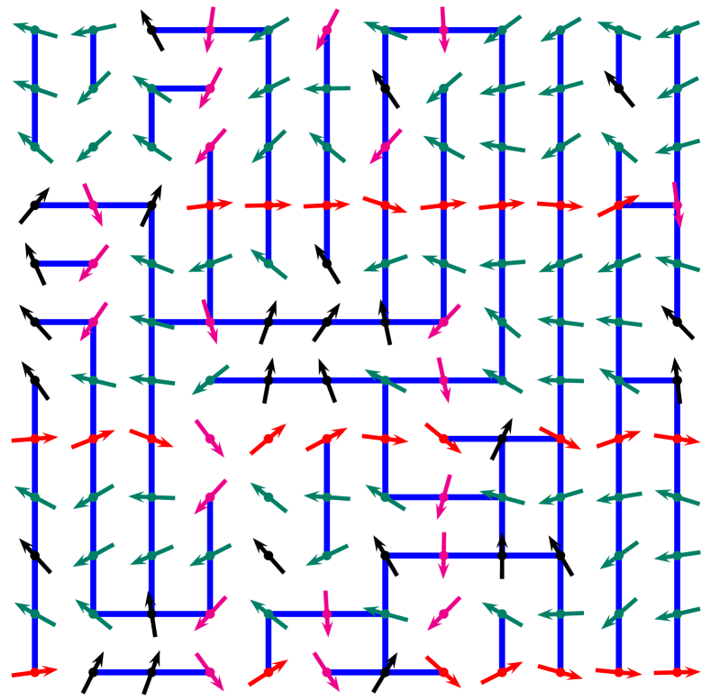
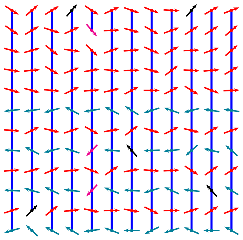
can be used to give a visualization and characterization of the different phases as in Fig. 1. On the lattice we thereby mark all bonds which have less than the average bond energy (those that contribute most to the partition function) and look at the global structure of the resulting bond clusters. In the disordered phase we expect rather random clusters whereas the ordered phase is characterized by clusters which are directionally ordered and independent of each other (dimensional reduction). Note, that in two dimensions $D$ and $D^{\prime}$ are actually the same quantity up to a constant factor, because $D=2D^{\prime}$. However, Eq. (4) provides the general possibility to define an order parameter in any dimension $d$, which might be useful for future studies. In order to investigate the universality class of the phase transition we further look at the susceptibility $\chi$ and Binder parameter $Q_{2}$ which are respectively defined as

$$\chi=N\left(\langle D^{2}\rangle-\langle D\rangle^{2}\right)\,,\quad Q_{2}=1-\frac{1}{3}\frac{\langle D^{4}\rangle}{\langle D^{2}\rangle^{2}}\,,$$ (5)

where $\langle D^{n}\rangle$ denotes an average of the $n$-th moment computed from the time series of $D$.

For the susceptibility we expect a finite-size scaling behavior of the form

$$\chi\sim L^{\gamma/\nu}\,,$$ (6)

at the critical point with $\nu$ being the correlation length critical exponent and $\gamma$ the exponent for the susceptibility. Neglecting corrections to scaling, the Binder parameters for different lattices sizes $L$ should ideally cross at the critical temperature $T_{\mathrm{c}}$. In any case, the behavior of the crossing points of $Q_{2}$ at lattice sizes $L$ and $2L$ should approach $T_{\mathrm{c}}$ like $L^{-1/\nu-\omega}$ if we have corrections to scaling ($w<\infty$).

II.2 Monte Carlo methods

Ordinary Metropolis Monte Carlo simulations are used for the classical model where we update each spin sequentially. During the thermalization procedure we adjust the proposed moves such that an average acceptance rate of about $50\%$ is obtained at each temperature. As it already becomes apparent from simulations on very small lattice sizes $L$ that the system suffers from huge autocorrelation times we add a parallel tempering (PT) schemeGeyer and Thompson (1995); Hukushima and Nemoto (1996), where we propose to exchange spin configurations between simulation threads at different temperatures $T_{i}$. This exchange is attempted every $n$ sweeps, where $n$ is typically in the range $2$ to $20$. By tracking individual configurations we make sure all temperatures are seen and that sufficient diffusion through temperature space is performed. For simplicity the simplest PT scheme is used, meaning that an equidistant temperature spacing between neighboring processes is chosen. As a result a reduction of autocorrelation times by two orders of magnitude is achieved which pays off in comparison to little longer simulation times.

In case of quantum spin degrees of freedom, we employ a quantum Monte Carlo (QMC) procedure based on the stochastic series expansion (SSE)Sandvik and Kurkijärvi (1991) technique originally developed by Sandvik. Our own implementation is based on the (directed) loop schemeSyljuåsen and Sandvik (2002) supplemented by ideas of Ref. Alet et al., 2005a. Recall that the principle of SSE is sampling the series expansion of the quantum partition function

$$Z =\mathrm{tr}\left(\exp(-\beta\mathcal{H})\right)=\sum_{\alpha}\sum_{n}\frac{(-\beta)^{n}\langle\alpha|\mathcal{H}^{n}|\alpha\rangle}{n!}\,,$$

$$=\sum_{b_{i}\in S_{n}}\sum_{\alpha}\sum_{n}\frac{\beta^{n}}{n!}\langle\alpha|\prod_{i}^{n}\mathcal{H}_{b_{i}}|\alpha\rangle\,.$$ (7)

by a Markov chain stochastic process, where $\beta=1/k_{\mathrm{B}}T$ is the inverse temperature. The last line of Eq. (II.2) is the central starting pointSandvik and Kurkijärvi (1991) of the method because it specifies the configuration space (and the weights) in which the sampling takes place. A configuration lives in the product space of spin configurations $|\alpha\rangle$ times the space of all possible sequences (or permutations) $S_{n}$ of $n$ bond operators (or vertices) $\mathcal{H}_{b_{i}}$. The degrees of freedom are thus $|\alpha\rangle$, $n$, and $S_{n}$, which are sampled by the usual combination of diagonal, non-diagonal, and spin flip updates.Syljuåsen and Sandvik (2002)

In the case of the compass model the bond operators $\mathcal{H}_{b_{i}}$ can be derived from the Hamiltonian (2) as

$$\mathcal{H}_{b}\in\begin{cases}S^{z}_{i}S^{z}_{j}&\text{if $b$ is a $z$ bond}\\ \{S_{i}^{+}S_{j}^{+},S_{i}^{-}S_{j}^{-},S_{i}^{+}S_{j}^{-},S_{i}^{-}S_{j}^{+}\}&\text{if $b$ is a $x$ bond}\,,\end{cases}$$

where the appearance of pure $S_{i}^{-}S_{j}^{-}$, and $S_{i}^{+}S_{j}^{+}$ terms are a notable difference to an ordinary Heisenberg model. Here $S^{+}$ and $S^{-}$ refer to creation and annihilation operators and the subscripts $i,j$ are the two sites of the bond $b$. Simulations of the quantum compass model are furthermore more involved since the Hamiltonian dictates an asymmetry between bonds in $x$ and $z$ direction, allowing no spin flip operators of type $S^{\pm}S^{\pm}$ to reside on $z$-bonds. On the other hand, there are a priori no diagonal terms $S^{z}S^{z}$ on $x$-bonds. However, since non-diagonal terms can only be introduced into the SSE configuration space after the diagonal-update (non-diagonal operators must be present!) we are therefore forced to introduce a positive non-zero energy shift $\epsilon$ into the Hamiltonian of Eq. (2). As a consequence both non-diagonal and diagonal terms may reside on $x$-bonds. On $z$-bonds only diagonal terms are allowed. Unfortunately, this asymmetry in the operator representation cannot be transformed away by a simple “symmetrizing” rotation of the Hamiltonian because of emerging minus sign problems. Note finally that the non-zero energy shift $\epsilon$ has an effect on the order parameter $D$ since it influences the number and the distribution of bond operators in the operator sequence. This effect can cause additional finite-size contributions also in the susceptibility and the Binder parameter which vanish in the thermodynamic limit and for $T\to 0$. We have checked that at $L=16$ no difference could be detected in the susceptibility maxima locations for $\epsilon=0.1,0.5,0.9$ within error bars. Here we work with $\epsilon=0.5$ at all lattices sizes.

Since simulations of the quantum model display the same rapid critical slowing down as the classical model we perform additional quantum PT updatesSengupta et al. (2002) in the same manner as described above. We implemented both the classical and quantum Monte Carlo PT scheme on parallel architectures with the restriction of shared memory access for fast communication between processes. This is essential since PT updates are done rather often.

For data analysis purposes we use well-known multi-histogram techniques to optimally combine simulations at different temperatures. Those techniques are available for both the classicalA. M. Ferrenberg and R. H. Swendsen (1989) and quantum casesTroyer et al. (2003, 2004). In combination with optimization routines like the Brent methodR. P. Brent (1973) they allow rather systematic and unbiased estimation of pseudocritical temperatures from peaks in the susceptibility.

II.3 Boundary conditions

\psfrag{l}{{\rm pbc}}\includegraphics[width=433.62pt]{pictures/pbc.eps}

\psfrag{l}{{\rm abc}}\includegraphics[width=433.62pt]{pictures/abc.eps}

Figure 2: (Color online) Visualization of the different boundary conditions used in this work. Left: Ordinary periodic boundary conditions. All bonds carry the same coupling and the dashed bonds connect the spins across boundaries. The topology is a torus. We refer to this case as pbc. Right: So called “annealed” boundary conditions (abc).Mishra et al. (2004) Here the sign of the couplings on the dashed boundary bonds may fluctuate dynamically resulting in an additional degree of freedom. As an example we draw some thick bonds indicating a negative coupling.

Figure 3: Data for the 2D classical compass model obtained by Monte Carlo simulations. The top row displays the results for periodic boundary conditions and the bottom row for annealed boundary conditions. Note the the temperature ranges are different for both cases and that not all lattice sizes are shown for better readability. The lines through the data points are obtained from the multi-histogram analysis. Left: The order parameter $D$ as a function of different lattice sizes $L$. Middle: The susceptibility $\chi$ of the order parameter. Right: The Binder parameter $Q_{2}$.

Ordinarily, the vast majority of Monte Carlo simulations are performed using periodic boundary conditions (pbc) which map the lattice onto a torus topology using the assumption that free-energy contributions from the surface are thereby minimized. In contrast to this approach, Mishra et al.Mishra et al. (2004) argue in their recent contribution that periodic boundary conditions might not be optimal in the case of the compass model. Instead, they introduce special, so called annealed boundary condition (abc) to arrive at their Monte Carlo results. Since a detailed comparison between these two boundary conditions has to our knowledge not been done, we will explicitly study and compare their effect on the finite-size scaling behavior for the classical compass model. This comparison is especially interesting in view of the fact that we may not easily apply the annealed case to quantum Monte Carlo since it induces a minus sign-problem. A characterization and understanding of the scaling behavior for periodic boundary conditions would therefore be of advantage before studying the quantum case.

Figure 2 displays these two types of boundary conditions as a sketch. The topology of the annealed boundary condition is the same as for periodic boundary conditions. The annealed case is special because the sign of couplings on bonds across the border may fluctuate dynamically according to the Boltzmann distribution. The bond sign is therefore an additional degree of freedom in the Monte Carlo update rendering the simulations somewhat more complex.

III The classical compass model in 2D

In this section we start the presentation of our simulation results. We consider firstly Monte Carlo simulations of the 2D classical compass model. The main purpose of this section is to give an explicit comparison between the different boundary conditions introduced in the last section. To this end we run simulations for both cases and compare the observables of Sec. II and their finite-size behavior. Figure 3 gives an overview of our Monte Carlo estimates for $D$, $\chi$ and $Q_{2}$. There, the top row contains results for periodic boundary conditions and the bottom row for annealed boundary conditions. Knowing the different behavior of reaching the thermodynamic limit is useful in order to appreciate results of our simulations which follow in subsequent sections.

Simulations are done using lattice sizes $L=\{10,12,16,24,32,36,48,64,128\}$ periodic bc and ${L=\{10,12,16,20,24,36,52,64\}}$ for annealed bc, typically taking about $10^{5}$ measurements per data point after an equilibration phase of $10^{4}$ sweeps. By the behavior of the order parameter in Fig. 3 (left) it is immediately evident that there is a phase transition and that directional order with $D>0$ is realized at low temperatures. We secondly observe that the order parameter for the pure periodic case has a slow convergence for small lattice sizes while for larger sizes it suddenly moves considerably. In contrast, the data for the annealed case show a much smoother movement towards the infinite-volume limit and it is evident that finite-size effects are drastically reduced. A difference like this is actually expected for different boundary conditions. The crucial and interesting question is whether the two boundary conditions lead to the same critical temperature in the infinite volume limit where boundary effects should vanish.

We therefore obtain an estimate of the critical point $T_{\mathrm{c}}$ in the thermodynamic limit by fitting the pseudocritical temperatures $T_{\mathrm{c}}(L)$ taken from the peaks of the susceptibilities in Fig. 3 (middle) at lattice size $L$ to the finite-size scaling ansatz

$$T_{\mathrm{c}}(L)=T_{\mathrm{c}}+bL^{-1/\nu}(1+cL^{-\omega})\,.$$ (8)

Here $b,c$ are some constants and $\omega$ is an exponent describing corrections to scaling. In a first step, we assume nothing about the value for the correlation length exponent $\nu$ and leave it as fit parameter.

Figure 4: (Color online) Determination of the critical temperature $T_{\mathrm{c}}$ from finite-size scaling of the pseudocritical temperatures determined from susceptibility peaks. The two curves correspond to different boundary conditions which trigger a completely different convergence to the critical point. The lower curve is obtained for annealed boundary conditions (abc) and shows the superior scaling compared to periodic boundary conditions (pbc). Lines are fits to Eq. (8) neglecting the correction term $\omega$.

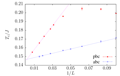
The fitting procedure to the data in Fig. 4 yields $T_{\mathrm{c}}=0.144(2)J$ from periodic boundary conditions and $T_{\mathrm{c}}=0.1461(8)J$ from annealed boundary conditions and the estimate for the correlation length critical exponent is $\nu=0.98(4)$ which we take from the straight line fit for the annealed case. Both results agree within error bars. The annealed value yields a much more accurate estimate since here the asymptotic scaling regime sets in much earlier and we have more points available for fitting. These numerical estimates are in accordance with the value $T_{\mathrm{c}}=0.147(1)J$ obtained in Ref. Mishra et al., 2004. With our value for $\nu$ we support the claim that the transition is of 2D Ising type. To further confirm this conjecture we also determine the exponent $\gamma$ associated with the susceptibility $\chi$. For lattice sizes large enough ($L>20$) we obtain $\gamma/\nu=1.73(4)$ from the annealed case (see Table 1 and Fig. 7 below) which is again consistent with 2D Ising universality. In a second step, we can now assume Ising universality to be given to improve the fit. Using $\nu=1$ as a fixed parameter the improved value for critical temperature is $T_{\mathrm{c}}=0.1464(2)J$.

Let us now turn to a discussion of the Binder parameter $Q_{2}$ displayed in Fig. 3 (right). For the annealed case a nice crossing of curves at the critical temperature can be observed and our estimate for the Binder parameter at the crossing point (taking the three largest lattice sizes) is $Q_{2}=0.61(1)$. This is roughly the known value for the 2D Ising model, which – however – is usually obtained for periodic boundary conditions.Kamieniarz and Blote (1993) Using the observed crossing behavior, the Binder parameter supplies a natural third check of the critical temperature and the critical exponent. We hence apply our recently developed data collapsing toolWenzel et al. (2008) and obtain $T_{\mathrm{c}}=0.1465(4)J$ and $\nu=1.01(4)$ from the best data collapse. These values are again fully consistent with our results above and give further confidence to our analysis. In contrast, the nice properties of the Binder parameter do not show up for periodic boundary conditions, where it is hard to judge whether curves for different lattice sizes cross in a single point at all. Rather, we see strong finite-size effects and that the crossing points for large lattice sizes move close to $2/3$, which is totally in contrast to the expected behavior. It is known that different boundary conditions cause a discrepancy (see for instance Refs. Kamieniarz and Blote, 1993 and Selke, 2006) in the Binder crossings but such a drastic behavior was unexpected.

In summary, our investigation for the classical model clearly show that annealed boundary conditions are favorable because they drastically reduce finite-size effects and yield good scaling properties for the finite-size analysis. With periodic boundary conditions much larger lattice sizes need to be investigated in order to obtain the critical temperature and to approach the right asymptotic scaling regime. Additionally, our analysis shows that the Binder parameter for periodic boundary conditions does not cross at the usual expected value and that we may not use the crossing point (height) as a good indication for the critical point, whereas for annealed conditions we get good properties. These effects are currently not properly understood. By referring to the typical spin configuration in Fig. 1 it is, however, tempting to argue that the dominant energy correlations (blue lines) wrap around the torus in the ordered phase thereby forming some kind of closed loop excitations. These excitation appear to be more stable against thermal fluctuations than open excitation. Annealed boundary conditions seem to prohibit the formation of such loops leading to a better scaling behavior.

IV The quantum compass model in 2D

Figure 5: QMC results for the 2D quantum compass model with periodic boundary conditions. All lines are a guide to the eye. (a) The order parameter $D$ for lattice sizes ${L=\{12,14,16,18,20,28,32,40,52,64\}}$ displays a clear signal of a stable ordered phase at low temperatures. The arrow marks the transition temperature $T_{\mathrm{c}}$ from Ref. Tanaka and Ishihara, 2007. Our own data indicates a smaller value. (b) The susceptibility $\chi$ on a logarithmic scale for lattice sizes $L=\{10,12,14,16,18,20,28,32,40,52,64\}$. (c) the Binder parameter $Q_{2}$ in the quantum compass model with periodic boundary conditions, where steeper slope corresponds to larger $L$ (neglecting $L=28$ and $L=48$ for better clarity). The qualitative behavior is the same as for the Binder parameter with periodic boundary conditions in the classical model. No common crossing point is present for the lattice sizes of this work.

Using the knowledge gained from simulations of the classical compass model we turn to the discussion of the simulation results of the quantum version. Simulations are done using the stochastic series expansion as outlined in Sec. II. The reader is reminded that annealed boundary conditions, where the sign on boundary bonds fluctuates, are not possible because such fluctuations induce a sign problem in the quantum Monte Carlo scheme.

We therefore choose to simulate with periodic boundary conditions and expect from Fig. 4 that large lattice sizes might be needed to see the right scaling and to obtain the infinite-volume critical temperature. Using the parallel tempering scheme and the reduction of autocorrelation times by two orders of magnitude, we were finally able to simulate lattice sizes ${L=\{8,10,12,14,16,18,20,24,28,32,40,48,52,64\}}$, where the largest one is about the limit one can reach in quantum Monte Carlo in feasible time and resources at the moment. Our largest system size is about three times as large compared to the simulations of Ref. Tanaka and Ishihara, 2007. A detailed check and verification of our algorithm was done with data from full exact diagonalization (ED) on a $4\times 4$ lattice. We use our own ED program with some implemented symmetriesDorier et al. (2005) to reduce the dimension of the Hilbert space, as well as the ALPS packageAlet et al. (2005b) for smaller system sizes. During the Monte Carlo runs, a total number of about $4\times 10^{5}$ measurements are typically taken after each sweep and $2\times 10^{4}$ sweeps are used for thermalization. Those numbers are, of course, only meaningful with the additional information that we construct as many loops in the non-diagonal update such that on average $2n$ vertices are visited in the SSE configuration. Figure 5 shows the result for the order parameter, the susceptibility and the Binder parameter obtained from the simulations in this manner. The behavior of the order parameter shows a clear signal of a transition from a disordered to an ordered state at small temperature, evidently becoming more pronounced with increasing lattice size. This proves the existence of a directional-ordering transition also in the quantum case. In the ordered phase, the order parameter seems to take on a value which is quite different from the classical case and the order is furthermore less stable against thermal fluctuations as the temperature regime in the quantum case is evidently much smaller. Note that the overall estimate for $D$ also agrees roughly with data of Ref. Tanaka and Ishihara, 2007.

The dependence of the data on the lattice sizes is, as expected, qualitatively similar to the classical case, i.e., the order parameter curves and the susceptibility peaks shift considerably to lower temperatures for larger lattice sizes. This shift is in fact so large that it is already obvious from Fig. 5 (a) that the previous estimate of the critical temperature in the literature is much to large.

Figure 6: (Color online) Finite-size scaling of pseudocritical temperatures for different lattice sizes obtained from the susceptibility. For small lattice sizes corrections to scaling are evident. For large lattice sizes 2D Ising scaling is reached yielding our estimate for the critical temperature of $T_{\mathrm{c}}/J=0.055(1)J$. The curve trough the points represents a fit to Eq. (8). We also show the crossing points of the Binder parameters at $L$ and $2L$ for a consistency check. The arrow indicates the previous result of Ref. Tanaka and Ishihara, 2007.

Figure 7: (Color online) Plot of the susceptibility $\chi$ (at peak locations) versus system size $L$ for all different simulations in this work (classical annealead bc, classical periodic bc, quantum periodic bc in this order from top to bottom) on a double logarithmic axis. The straight lines are fits to Eq. (6). All cases are consistent with a value of $\gamma/\nu=1.75$.

Before we quantify this discrepancy for the critical temperature, we draw our attention to the susceptibility and the Binder parameter in Figs. 5(b),(c), both showing a behavior similar to the classical case with periodic bc. We note especially that the Binder parameter is again behaving oddly and that there is not a well defined crossing seen at all at the lattice sizes simulated. A crossing point might still be achieved for very large lattice lengths $L$ but is certainly difficult to quantify since the value of $Q$ at the crossing point is very close to $2/3$. Due to this observation the Binder parameter is clearly not suited to determine the critical temperatures by looking at the Binder crossings for small lattice sizes, where the true behavior is just not seen.

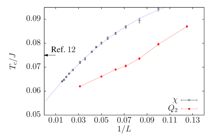
Let us now determine an improved value for the critical temperature with finite-size scaling from the maxima of the susceptibilities. As in the classical case, we fit the pseudocritical values to the scaling ansatz given in Eq. (8). To use as many data points as possible we include corrections to scaling, described by the exponent $\omega$, into the fit and leave all fit parameters free. Including all lattice sizes we obtain $T_{\mathrm{c}}=0.055(6)J$ and $\nu=0.9(2)$ with a fit quality of $\chi^{2}/\mathrm{d.o.f}=0.66$. Those values, however, are stable also for fitting windows starting at larger lattice sizes. The precision for the critical exponent $\nu$ is rather low but agrees with our expectation of 2D Ising universality within the error bar. Under this assumption, we fix $\nu=1$ and repeat the fit procedure yielding an improved estimate for the critical temperature as $T_{\mathrm{c}}=0.055(1)J$. The relative discrepancy with the previous estimate of Ref. Tanaka and Ishihara, 2007 is approximately $36\%$. As a cross check for our analysis we further look at the scaling of the crossing points of $Q_{2}$ at lattice sizes $L$ and $2L$, which is also indicated in Fig. 6. We observe that this scaling is consistent with the previous value from the susceptibilities but we do not attempt a detailed fit by lack of enough data points. It is then also useful to obtain an independent estimate of the critical temperature from the maxima in the heat capacity $C$, which again gives consistent results but does not reach the accuracy of our previous analysis since $C$ is generally hard to sample in QMC at low temperatures.

To finalize our analysis, we determine the critical exponent $\gamma$ from the susceptibility of the order parameter $D$. For large lattice sizes we expect a scaling according to Eq. 6 which can be tested by plotting $\ln(\chi)$ versus $\ln(L)$. This is done in Fig. 7 together with the data for the classical cases. It is evident that asymptotic scaling sets in only for the largest lattice sizes from which we obtain a value of $\gamma/\nu=1.68(8)$ consistent with 2D Ising universality, but not precise enough to be absolutely conclusive.

V Summary and Conclusions

Table 1: Results for the critical temperature and critical exponents as obtained in this work. The upper section contains the results for the classical model taken from annealed bc, which are all pairwise consistent. The middle section summarizes our estimates for the quantum compass model for the cases with and without the assumption of 2D Ising behaviour ($\nu=1$). Both cases are consistent with each other. Lastly the values for $\gamma/\nu$ are summarized as obtained from the largest lattice sizes for the different simulation runs.

	$T_{\mathrm{c}}/J$	$\nu$	$\omega$	$\chi^{2}/\mathrm{d.o.f}$
no assumption	$0.1461(8)$	$0.98(4)$	$-$	$1.3$
2D Ising	$0.1464(2)$	$-$	$-$	$1.15$
collapse $Q_{2}$	$0.1465(4)$	$1.01(4)$	$-$	$-$
no assumption	$0.055(6)$	$0.9(2)$	$0.5(4)$	$0.66$
2D Ising	$0.055(1)$	$-$	$0.8(2)$	$0.61$
	class. (abc)	class. (pbc)	quant. (pbc)
$\gamma/\nu$	$1.73(4)$	$1.72(5)$	$1.68(8)$

In this paper we reported on comprehensive Monte Carlo simulations of the classical and quantum compass model. By comparing different boundary conditions for the classical case, we showed that for ordinary periodic boundary conditions one needs to go to very large lattice sizes to see the right scaling and to get good convergence to the critical point. In order to simulate large lattice sizes, we implemented a parallel tempering scheme to counteract huge autocorrelation times. Our results, which are summarized in Table 1 are perfectly consistent with previous studies in the literature for the classical model. For the quantum model our simulations are quantitatively at odds with earlier studies and we provide here a new estimate for the critical temperature $T_{\mathrm{c}}$. We argued that this discrepancy might be explained by the huge finite-size corrections originating from stable loop excitations formed by correlation orderings which appear on the torus topology at periodic boundary conditions. It appears that those excitations even destroy the usual properties of Binder parameters. Our analysis, however, shows that one can still arrive at an estimate for $T_{\mathrm{c}}$ at periodic boundary conditions provided that one takes this effect into account. All critical exponents obtained in this study give further support to the claim that 2D Ising universality describes the directional-ordering transition in the 2D compass model.

Our findings for the quantum model might have an impact on the conclusions of Ref. Tanaka and Ishihara, 2007 because a precise estimate of $T_{\mathrm{c}}$ enters into the analysis of dilution effects on the model. It is conceivable that the conclusion obtained there are still qualitatively valid. For a true quantification of the dilution effect, however, there is no way around performing a more detailed investigation of larger lattice sizes. The knowledge gained in this work should help to start such a study.

The precision of our results for the quantum model are still rather low compared to many other systems of statistical physics. In this respect it would be an interesting future project to devise and analyze special boundary conditions for the quantum model with improved finite-size scaling behavior compared to periodic boundary conditions.