NEMO-O$\nu$DE : a submarine station for real-time monitoring of acoustic background installed at 2000 m depth in the Mediterranean Sea

Abstract

The NEMO (NEutrino Mediterranean Observatory) Collaboration installed, 25 km E offshore the port of Catania (Sicily) at 2000 m depth, an underwater laboratory to perform long-term tests of prototypes and new technologies for an underwater high energy neutrino km³-scale detector in the Mediterranean Sea. In this framework the collaboration deployed and successfully operated for about two years, starting form January 2005, an experimental apparatus for on-line monitoring of deep-sea noise. The station was equipped with 4 hydrophones and it is operational in the range 30 Hz - 43 kHz. This interval of frequencies matches the range suitable for the proposed acoustic detection technique of high energy neutrinos. Hydrophone signals were digitized underwater at 96 kHz sampling frequency and 24 bits resolution. A custom software was developed to record data on high resolution 4-channels digital audio file. This paper deals with the data analysis procedure and first results on the determination of sea noise sound pressure density curves. The stored data library, consisting of more than 2000 hours of recordings, is a unique tool to model underwater acoustic noise at large depth, to characterise its variations as a function of environmental parameters, biological sources and human activities (ship traffic, …), and to determine the presence of cetaceans in the area.

, , , , , , , , , , , , , , , , , , , , , , , , , , , , , , , , , , , , , , , , , , , , , , , , , , , , , , , , , , , , , , , , , , , , , , , , , , , , , , , , , , , , , , , , , , , , , , , , , .

1 Introduction

In recent years the astrophysics and particle physics Community strongly addressed its efforts in the realization of large experimental apparatuses with the goal of detecting high energy neutrinos ($E_{\nu}>10^{12}$ eV) originated in cosmic sources GaisserHalzenStanev1995 . The detection of these particles will open a new window in our comprehension of the Universe and in the understanding of physics processes occurring in powerful cosmic sources such as Active Galactic Nuclei Mannheim1995 , Gamma Ray Busters WaxmanBahcall1997 , microquasars Distefano2002 and Supernova Remnants Vissani2005 .

The experimental techniques proposed to identify the cosmic neutrino signatures are mainly three Markov1961 : the detection of Čerenkov blue light originated by charged leptons (electrons, positrons, muons and tauons) from a neutrino interaction in water or ice; the detection of acoustic waves produced by neutrino energy deposition in water, ice or salt; the detection of radio pulses following a neutrino interaction in ice or salt.

Due to the faintness of expected astrophysical neutrino fluxes (about 10⁶ particles per km² per year, following a $E^{-2}$ spectrum), and due to the extremely low probability of neutrino detection in the detector volume ($\simeq 10^{-4}$), the required size of these apparatuses is about 1 km³ for neutrinos of energy $10^{12}\div 10^{15}$ eV and more than 10 km³ for more energetic particles. The only way to build such a detector is the use of large natural media such as seawater, polar ice or lake freshwater. Moreover all these techniques require that the detector must be placed at large depth underground (about 1000 m), undersea or under ice ($>$3000 m) to shield the detector from the intense background of cosmic particles that would cancel the neutrino signal. The Čerenkov technique is presently in a mature phase. The first km³ scale detector is under construction at the South Pole Icecube .The activity in the Mediterranean Sea in presently focused in the construction and operation of prototypal, small scale detectors: ANTARES Carr2006 , NEMO Migneco2006 and NESTOR Resvanis2006 , technological demonstrators for the future Km3Net Km3Net , whose construction is planned between 2009 and 2012.

The NEMO Collaboration is strongly involved in the design and construction of the Mediterranean km³ Čerenkov neutrino detector. In the same time the Collaboration is starting studies on the acoustic detection technique; the first task, in this framework, was the measurement and monitoring of the acoustic background at large depth to evaluate the expected signal to noise ratio. At present, only few measurements of acoustic noise have been carried out at very large depth, where acoustic detectors should be presumably located. This is mainly due to technological difficulties in constructing, deploying and operating real-time monitoring stations in deep sea. Noise in the sea has different origins: biological (fishes, marine mammals, crustaceans), seismic and micro-seismic, mechanical (wind and surface waves), molecular thermal vibrations and human activities (navigation, fishing, military operations, oceanographical instrumentation, oil exploration). Biological and human noises could reach very high pressure level, but they are, generally, produced by local and intermittent sources. At large depths it is expected that surface agitation noise (which is the major source of noise in the kHz range) should be reduced due to the change of sound refraction index with depth. On the other hand, it is not well known the contribution of sound emissions generated by cetaceans, that can immerse down to thousand meters depth Pavan2000 . Bibliographic data indicate that, in the frequency range of interest for neutrino detection (10 $\div$ 100 kHz), the acoustic noise in water is a sum of a diffuse and relatively steady background due to ship traffic and sea state conditions that occasionally add up with loud and transient sources, such as biological sounds (dolphin and whale vocalizations), and man-made noise (close ships, navigation and scientific instrumentation: pingers, air-guns) Urick .

In order to measure the level of acoustic noise in the deep Mediterranean Sea, the NEMO Collaboration constructed and operated the experimental station O$\nu$DE (Ocean noise Detection Experiment), a real-time experiment to monitor acoustic signals in deep sea.

2 The physics case

Underwater Čerenkov telescopes for high energy neutrinos are arrays of large-area photomultipliers (PMTs), having typically 10 inches diametre, designed to detect Čerenkov blue light radiated in water by charged leptons from neutrino Charged Current interactions. The reconstruction of the Čerenkov tracks allows the identification of the lepton direction and energy thus, to some extent, the neutrino direction and energy. The effort of the astro-particle physics community is presently addressed in the construction of two detectors (Km3Net Katz2006 in the Mediterranean Sea and ICECUBE Achterberg2007 in the Antarctic ice-cap) equipped with some thousands of PMTs. These detectors are expected to reach detection areas of about 1 km² at E${}_{\nu}=$ 1$\div$100 TeV and to identify astrophysical point-like neutrino sources and measure the high energy diffuse cosmic neutrino flux. At higher energies ($>10^{16}$ eV) however, the expected neutrino fluxes are fainter (the spectrum follows a $E_{\nu}^{-2}$ power law), and detectors with detection areas $>$10 km² are required. A different detection technique was suggested Askarian1957 to build larger detectors. At these energies neutrino interactions in water produce showers, that release instantaneously a macroscopic amount of energy in a small cylindrical volume of matter. Ionization and sudden heating of water produce a bipolar pressure pulse which expands perpendicularly to the shower axis. The maximum wave amplitude, calculated with thermo-acoustic models, scales linearly with the density of energy deposition: for a 10²⁰ eV neutrino induced shower it is few tens mPa at a distance of $\sim$ 1 km from the shower axis Vandenbroucke2005 . The wave peak frequency is estimated to be in the range of 10 kHz. The advantage of acoustic detection is the long absorption length of sound in water: in this frequency range, it is of the order of few kilometres. A pioneering work on acoustic neutrino detection has been recently conducted using military arrays of hydrophones Lehtinen2002 .

Due to the small amplitude of the expected neutrino bipolar signal, it is mandatory to measure the acoustic noise in the sea as a function of frequency in order to study the performances of a future acoustic detector as a function of the number of sensors and of the design of the antenna. This was the main goal of O$\nu$DE . The detector was deployed during January 2005 at the INFN Laboratori Nazionali del Sud (LNS) deep sea Test Site, located at depth of $\sim$ 2000 m, 25 km E offshore the port of Catania (Sicily), see Figure 1. The detector acquired data from January 2005 to November 2006, when the NEMO Collaboration started to install the NEMO Phase 1 detector: a technological demonstrator for the future km³ Čerenkov neutrino telescope Migneco2006 .

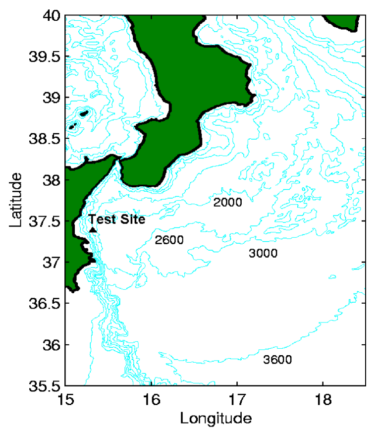
Figure 1: Bathymetric chart of the Eastern Sicilian Coast region. The location of the Catania TSS (triangle) is shown. The O$\nu$DE frame is moored at 2050 m depth, latitude $37^{\circ}30^{\prime}008$ N and longitude $015^{\circ}23^{\prime}034$ E.

3 The Catania Test Site infrastructure

The Catania Test Site consists of a shore laboratory, a 28 km long electro-optical (hereafter e.o.) cable connecting the shore lab to the deep sea lab. The shore laboratory hosts the land termination of the cable, the on-shore data acquisition system and power supplies for underwater instrumentation. The underwater cable is an umbilical underwater e.o. cable, armored with an external steel wired layer, containing 10 optical single-mode fibers (standard ITU-T G-652) and 6 electrical conductors (4 mm² area). At about 20 km E from the shore, the cable is divided into two branches, roughly 5 km long each, that reach two different sites namely Test Site North (latitude $37^{\circ}30^{\prime}810$ N, longitude $015^{\circ}06^{\prime}819$ E depth 2100 m), and Test Site South (latitude $37^{\circ}30^{\prime}008$ N, longitude $015^{\circ}23^{\prime}034$ E, depth 2050 m). The Test Site North (TSN) cable branch has 2 conductors and 4 fibres directly connected to shore, the Test Site South (TSS) branch has 4 conductors and 6 fibers. After deploying the main underwater cable, in January 2005 the Collaboration installed, on TSS and on TSS, two underwater frames. Each frame, made of grade 2 titanium, is equipped with a pair of e.o. connectors (see figure 2). The two frames were deployed on the seabed. The e.o. connectors are made to be handled by underwater robots ROV (Remotely Operated Vehicles) to allow plugging and unplugging of underwater experimental apparatuses, avoiding further recovery operations of the main cable. During the same naval campaign two experimental apparatuses were deployed, plugged and put in operation. The seismic and environmental monitoring station Submarine Network 1 (SN-1), designed and operated by the INGV (Istituto Nazionale di Geofisica e Vulcanologia, Italy) Favali2005 ; Favali2006 was connected to the TSN termination. This station is presently the only cabled node of the ESONET (European Seafloor Observatory NETwork) project ESONET . In January 23^th 2005 the O$\nu$DE station was deployed and connected to the TSS termination.

Figure 2: The titanium frame installed on TSS. The ROV operable electro-optical connectors are visible on the front panel. The hydrophones and electronics housing of the O$\nu$DE station are also shown (see text).

4 The O$\nu$DE apparatus

O$\nu$DE was designed to perform on-line monitoring of the acoustic noise at large depth. The station is equipped with four large bandwidth hydrophones (30 Hz - 50 kHz). Each hydrophone (hereafter H1,H2 H3 and H4) was mounted on an aluminum alloy vessel, pressure resistant, which also hosted the hydrophone preamplifier. The analog signals from the preamplifiers were transmitted, through underwater cables suitable for audio applications, to signal conditioning and digitization electronics hosted in a pressure-proof glass housing. Underwater, digital signals were translated into optical and sent to shore through the optical fibers. On shore, acoustic data were reconverted into electrical and recorded using a PC, in which a pair of professional PCI audio boards were mounted. Electrical power was supplied from shore.

4.1 Mechanical set-up

The mechanical structure of O$\nu$DE is composed by: a commercial pressure-proof glass housing (which hosts the DAQ and power supply electronics), one electro optical cable that connects the station to the e.o. plug mounted on the frame and four electrical cables that connect the housing to the four hydrophone vessels.

The vessels containing the hydrophone preamplifiers were made in aluminum alloy (Al-7075). The vessels are cylindrical with trunk-conical shaped terminations (angle 45^∘). This shape was chosen to fit the hydrophone body and to minimize the reflections of acoustic waves towards the hydrophone. A penetrator at the base of the aluminum vessel was designed and constructed to insert the electrical cable that connects the vessel with the glass housing (see Figure 3).

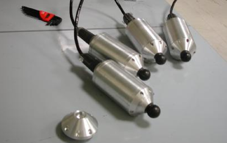
Figure 3: The Al-alloy housing that hosts preamplifiers and holds the hydrophones.

The hydrophones vessels were hooked on the upper part of the TSS frame, forming a tetrahedral antenna of $\sim$ 1 m side. The hydrophone vessel H3, was mounted in the highest position, close to the frame apex, that is at about 3.2 m above the seabed. Since most of the noise comes from above (the station is moored on the seabed) H3 was used as pilot hydrophone during signal analysis. H1,H2 and H4 were attached approximately at the same height (about 2.6 m above the seabed), in the squared upper edge of the frame. In picture 2, H1 is visible on the right with respect to the instrument housing (the orange spherical shell), H2 is placed behind the shell and H4 on the left. The glass housing is a commercial 17” diametre sphere, manufactured by Nautilus Nautilus . The sphere is made of two halves: the electronics was placed inside the sphere and, before deployment, the two halves were sealed together slightly de-pressuring to 750 mbar the cavity of the sphere, in a nitrogen filled environment. This pressure ensures both the sealing and the circulation of nitrogen inside the sphere, thus the cooling of the electronics. The sphere was equipped with 5 titanium connectors. One is an electro-optical dry-mateable connector, holding 3 optical and 2 electrical contacts. This connector was used to link the station to the frame e.o. connectors, by means of an electro-optical harness cable. The harness was terminated on one side with a dry mateable-plug, on the other with a ROV-mateable connector that matches the one installed in the frame. The other four electrical connectors were used to link independently each hydrophone to the electronics glass housing.

In order to get the absolute orientation of the frame (thus the orientation of the station), and in order to monitor the possible movements of the frame with respect to seabed, a tilt-meter and compass board (EZ-Compass-3, manufactured by Advanced Orientation System AOSI ) was installed inside the electronics glass housing of O$\nu$DE . The compass was equipped with an RS-232 communication port, which allowed board initialization, calibration and serial data transmission. The compass board was connected to shore through an optical bi-directional WDM optical link. The compass indicated that the frame had an orientation of about 108 $\pm$2 degrees with respect to North and it was laid almost co-planar ($5^{\circ}\pm 2^{\circ}$ roll, $-3^{\circ}\pm 2^{\circ}$ pitch) with the seabed. These values where confirmed by ROV inspections after the deployment and have not changed during the whole period of data taking.

4.2 Hydrophones and pre-amplifiers

We used RESON Reson TC-4042C hydrophones, derived from the TC4037 Series and tested by the manufacturer to operate at 250 bar pressure for long term deployment. The used hydrophones are piezoelectric sensors, having a mean receiving sensitivity of -195$\pm$3 dB re 1V/$\mu$Pa, linear over a wide range of frequencies: from few tens Hz to about 50 kHz. The hydrophone analog output is differential. The TC-4042C hydrophones were mounted on the channels H1,H2 and H3. A hydrophone from a different series, having a sensitivity 5 dB lower, was mounted on channel H4. All hydrophones have an omnidirectional directivity pattern suitable for ambient noise measurements, which is the purpose of the experiment. The hydrophone output signal was feeded into a preamplifier, developed also by RESON, which has a gain of 20 dB. Two preamplifiers (namely the ones installed on channels H2 and H4) were modified applying a hi-pass filter ($>$ 1 kHz, 6 dB per octave) to reduce the expected ambient noise, which has typically $1/f$ spectrum. This was done to avoid possible saturations due to the low frequency noise and to focus the measurements to the frequency range interesting for neutrino detection ($>$10 kHz). On the other hand the use of a pair of unfiltered large-bandwidth hydrophones (H1 and H3) allowed comparison with bibliographic data, which is more abundant for low frequency measurements.

4.3 Data digitization and transmission electronics

The differential output of each preamplifier was sent to a pair of line-output and line-input transformers. Line transformers were used to galvanically insulate the lines in case of shorts inside the hydrophone vessels and to balance the audio line. The line-output transformer was hosted inside the aluminum vessel, the line-input transformer inside the glass housing. The electrical line between the transformers, 4 m long, was a shielded twisted-pair cable suitable for analogue audio signal transmission.

The hydrophones signals were then sent to two stereo Analog to Digital Converters (ADC). Signal digitization was performed using Crystal CS5396 stereo ADCs Crystal . In particular channel H1 and H3 were plugged in the left and right channel of one board respectively, H2 and H4 (modified applying a $f>$1 kHz hi-pass filter, 3 dB per decade) were plugged to the left and right channels of the other board. The two ADCs received the same 12.288 MHz clock, thus they were synchronised. The CS5396 is a sigma delta ADC which samples the analog data at a rate of 96 kHz with a resolution of 24 bits, the input voltage range of the ADC is 4 V${}_{\hbox{PP}}$. The ADC outputs were sent to a Digital Interface Transmitters Crystal CS8404A that converted the data stream into standard SPDIF (Sony Philips Digital Interface Format) stream. The SPDIF protocol contains, together with data, the sampling time information; since the two ADCs and the two digital audio transmitters were driven by the same common clock the two stereo streams are synchronized. Since we know the phase response of the $>1$ kHz hi-pass filters applied on H2 and H4, the whole array can be also phased. This feature is extremely useful for TDoA (Time difference of arrival) analysis of signals detected by the four hydrophones, in order to recover the direction of emission of the detected sounds. The two output streams were sent to a pair of electro-optical media converters capable to transmit data over $\sim$ 50 km single mode optical fibre.

4.4 Power Supply

Power was supplied to the station from shore using stabilized 220 V${}_{\hbox{ac}}$ 50 Hz supplier and it was elevated in order to feed the station constantly at about 380 V${}_{\hbox{ac}}$. Taking into account the cable impedance, the voltage at shore was set, by means of a VARIAC, to about 415 V${}_{\hbox{ac}}$. A zero crossing switch was also used on shore to start power transmission only when voltage sinusoid was rising and close to zero. The power supply system was realised using all linear components, avoiding switching power converters which could cause electrical and mechanical noise in the interesting frequency band. Moreover all electronic components were galvanically insulated one from the other to avoid propagation of short-circuits through the power chain. Inside the deep sea housing we placed independents ac/ac power transformers, rectifiers and regulators to supply electronics at different dc currents (14 V${}_{\hbox{dc}}$ and 5 V${}_{\hbox{dc}}$), and to separate the power lines of analogue electronics from the digital ones. The underwater power distribution was made using low drop-out regulators to minimize power dissipation: the transformation efficiency was $\sim 70\%$ and the total power consumption, at 380 V${}_{\hbox{ac}}$ supply, was about 20 W. The temperature recorded close to the ADCs, by a thermometer mounted on compass board, was during the whole operation period, 26.2$\pm$0.2 ^∘C, when the sea temperature was 13.8$\pm$0.1 ^∘C.

5 On shore data acquisition

On shore, data from the underwater station were re-translated into electrical audio SPDIF (Sony Philips Digital Interface Format) standard using a pair of fiber optical data receivers. The two SPDIF stereo data stream are then addressed to a PC (Pentium IV, 3 GHz, 1 GB RAM) equipped with two professional PCI audio boards, RME DIGI96-8 PAD RME . In this sections the data acquisition/recording software and the file archiving strategy are described.

5.1 Software tools

Data acquisition on shore was performed, from January to April 2005, using standard 16 bits audio software tools and sampling independently the two pairs of hydrophones (H1-H3 and H2-H4). From May 2005 we used a custom software tool SeaRecorder developed by CIBRA CIBRA running under Windows XP. The program reads and keeps synchronized the two digital stereo data streams coming from the underwater station. Data, received in SPDIF format at 24 bit resolution and 96 kHz sampling frequency, are saved into standard Microsoft .wav 32 bit float format (24+8 bit). This format was chosen to allow data porting to Matlab matlab for off-line analysis.

SeaRecorder permits both data recording with floating point format or integer (16 or 32 bit/sample), and digital amplification of data at several gain factors. During acquisition, the software displayed average and peak values measured by the 4 channels and plotted, in real time, their envelope to provide on-line monitoring of the recording. The program also generated a log text file containing complete information of the software settings, average and maxima values measured for each recording. In figure 4 the data acquisition window of the used software is shown.

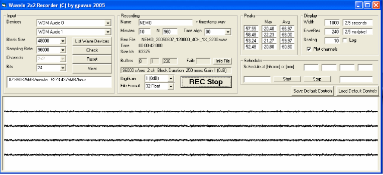
Figure 4: The main window of the SeaRecorder program, used to record and monitor data coming from the four hydrophones installed on O$\nu$DE

File recording can be programmed to be continuous, with automatic file splitting every hour or every 30 minutes, or scheduled for predefined file duration. A special filenaming protocol was adopted to reduce the risk of data losses or data misinterpretation. Filenames included a date-and-time stamp, number of channels, recording gain (linear), file format; sample rate was omitted as it was a hardware-locked parameter (96 kHz); a typical filename was therefore ONDE_20050827_161500_4CH1X_3200.wav.

An additional software tool, the SeaPro also developed by CIBRA, was used to read off-line the 4 channels, 32 bit, 96 kHz .wav files recorded by SeaRecorder to permit detailed data visualization. Two channels (selectable among the four) can be played as sounds and visualized as spectrograms (time vs. frequency diagrams) in the same time, allowing identification and classification of different sounds.

5.2 Data archival

After the experiment start-up, the data were continuously recorded for about one month, this allowed to evaluate the average value and variability of sound level and to define the successive strategy for scheduled recording. Continuous recording strategy was not possible due to storage space constraints: the amount of data sent to shore requires about 124 GB/day. Data were therefore recorded for five minutes (randomly chosen) continuatively every hour, this was a compromise to save a representative sample of unbiased data, reducing disk space consumption: the storage space required daily for 4 channel recording at 32 bits was 10.2 GB. A larger sample of data (about 20’ per hour) coming from H3 only, was also recorded using 16 bit file format.

The data sample presently analysed amounts to $\sim$ 1200 hours, covering 16 months from January to December 2005, and from July to November 2006. From mid February to the end of March 2005, and from January to June 2006, the station was not in operation due maintenance of the e.o. main cable and on-shore hardware. As explained in the following, the present paper deals with data recorded from May 2005 on.

6 Data analysis

As previously described, data from the four hydrophones were recorded as 4 channels .wav files at 24 bits and 96 kHz. This permitted offline data analysis under Matlab environment.

In figure 5 two seconds of data, recorded on 14 November 2006 at h 23:30, are shown, as an example. The amplitude values of the four channels, separately displayed, are in V (the ADC input range was between -2V and +2V). A biological sound is shown in figure 5: the click produced by a sperm whale (a signal emitted for echo-location) and its reflection on the sea surface. A software notch filter ($f=50$ Hz, $\Delta f=50/35$ Hz, -10 dB, the same for all channels) is applied to cut off the 50 Hz noise picked up from the power system. The highest spectral components of sea noise appear at $f<1$ kHz, thus they are filtered out in channels H2 and H4. The electrical signal amplitude corresponding to the click, recorded by H1,H2 and H3 is roughly the same, the signal in H4 is about 5 dB smaller, as expected.

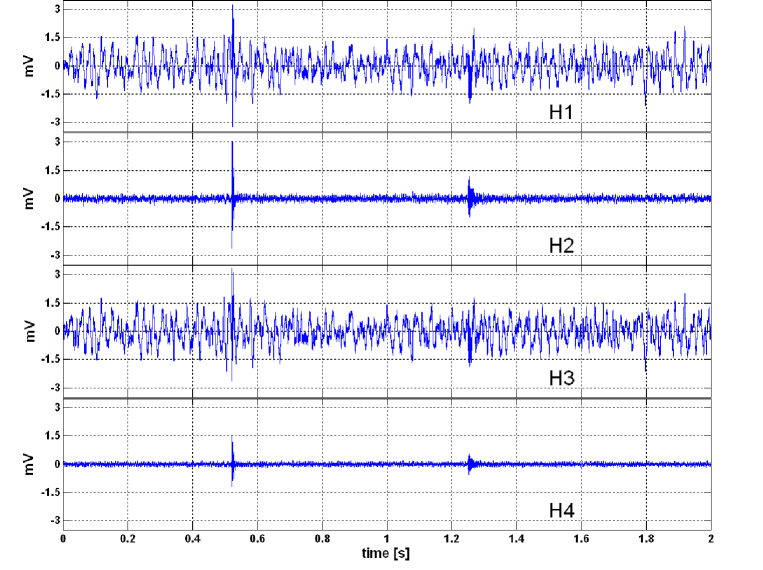
Figure 5: Example of recorded raw data (only 50 Hz noise filtered): a sperm whale click (occurring at $\sim$ 0.5 s) and its reflection on the sea surface (occurring at $\sim 1.3$ s). The four hydrophone channels are independently displayed. H2 and H4 had a hardware hipass filter $f>$1kHz and the whale click is clearly visible.

In order to determine the spectral Sound Pressure Density (SPD) of sea noise, the Power Spectral Density (PSD) of the signal is calculated per each recorded file (5’ recording = 300$\cdot f_{s}$ samples) :

$$PSD(f)=\frac{|X_{N_{DFT}}|^{2}}{f_{s}\cdot L}$$ (1)

where $f_{s}$ is the sampling frequency (96 kHz), $L$ is the time length of the signal (in units of seconds), and $X$ is the $N^{th}$ component of the Discrete Fourier Transform (DFT) corresponding to the frequency $f$. The file is divided into blocks of 2048 samples, weighted using an Hanning window and an overlap of 50$\%$ (i.e. a 1024 samples shift). The 2048 points Discrete Fourier Transform ($\Delta f\simeq 47$ Hz) is then calculated using the Fast Fourier Transform algorithm implemented on Matlab. Eventually we calculated the average, minimum and maximum values and the $30^{\hbox{th}}$, $50^{\hbox{th}}$, $90^{\hbox{th}}$ and $95^{\hbox{th}}$ percentile of the distribution of the obtained PSDs.

The analysis presented in this paper was carried out using only the data sample recorded with H3, from May to December 2005 and from July to November 2006 ($\sim$ 6400 files). Other data are not included in this paper, because they were taken using 16 bits recording software, so they are not homogeneous with the rest of the sample.

6.1 Determination of the detector electronic noise floor

Figure 6 presents the limits of variations of the average PSD distributions (grey area) obtained analysing $\sim$6400 files recorded by the hydrophones H3. Data for $f>43$ kHz (0.45 $f_{s}$) are not shown. The plot shows large variations in recorded signal amplitude, mainly for $f<$20 kHz, and a baseline that represents the RMS power of the electronic noise of our detector. This is a white noise for $f>5$ kHz recorded when the contribution of acoustic sea noise was very low. As shown later, it is due to the self noise of the hydrophone and the preamplifier, being the power of the ADC noise negligible (few nV²/Hz). The black dash-dotted line in figure 6 represents the average of PSDs over the whole data sample.

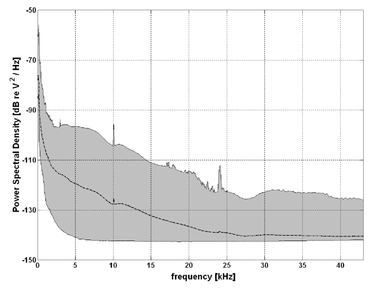
Figure 6: The grey area represents the upper and lower limits of average PSDs calculated for the $\sim 6400$ files of data (the file time duration is 5’) recoded using channel H3. The black curve is the average calculated over all PSDs.

The average (in blue) and the minima (in red) of average PSD curves calculated for different months with H3 are shown in figure 7. While the average curves change for different months, the minimum ones are very similar and almost independent on the frequency, for $f>$5 kHz. This behaviour indicates that minima are related to the electronics noise of the detector (hydrophone coupled to the preamplifiers).

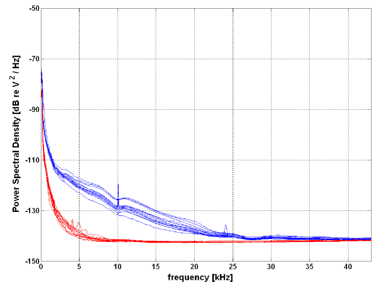
Figure 7: Averages (blue lines) and minima (red lines) of Power Spectral Density calculated, for each month, using channel H3 data. The minima curves are nearly superimposed: differences appears only at $f<5$ kHz, in months showing a high acoustic background.

The same results are observed in all the channels: figure 8 shows the minima (solid line) and average (dashed line) curves calculated using the data recorded in August 2005 for H1 (black) and H3 (red) respectively.

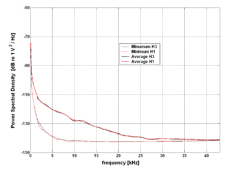
Figure 8: Average (dashed line) and minimum (solid line) PSD curves calculated for about $740$ files of data recoded during August 2005 with H3 (red) and H1 (black).

In order to demonstrate the correlation between PSD (Power Spectral Density) minima and electronic noise, the equivalent sound pressure density of the PSD minima curves was calculated, as shown in figure 7. The SPD (Sound Pressure Density) curves, shown in figure 9 were obtained multiplying PSD minima times the squared average sensitivity of channel H3 (-195 + 20 dB re 1 V/$\mu$ Pa), assumed flat in frequency. For $f>$5 the equivalent sound pressure density of PSD minima is $\simeq 33\pm$ 0.3 dB re $\mu$Pa²/Hz. In this range of frequencies the curves correspond in value and shape to the power of the self noise estimated by the manufacturer for a typical RESON TC4037 hydrophone and preamplifier set-up for $f>$5 kHz Reson . At lower frequencies this white electronics noise adds up with the noise induced by the power supply and with the acoustic background (not negligible at frequencies $\leq$ 1 kHz).

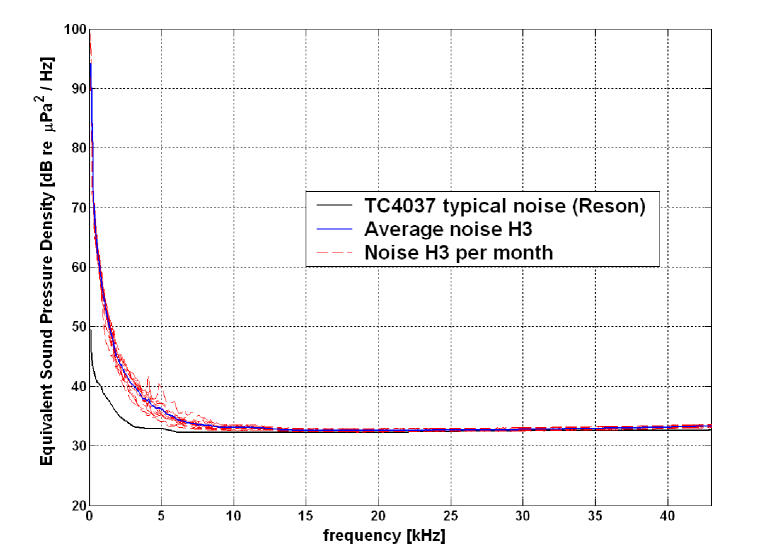
Figure 9: Equivalent sound pressure density of PSD minima calculated for each month (red dashed lines) and their average value (blue thick line). The equivalent noise curve provided by RESON for a typical TC4037 hydrophone is shown for comparison (black curve). The value of the minimum curve at $f>5$kHz ($\simeq 33\pm 0.3$ db re 1 $\mu$Pa²/Hz) corresponds to the RMS of equivalent noise power for a typical RESON TC4037 hydrophone and preamp acquisition system.

Since the electric signal produced by acoustic sea noise sums incoherently with the electronics noise, the sound pressure density of sea noise was recovered subtracting the average power spectral density curve of noise from the PSD of the signal.

We also took the standard deviation of the power spectral density minima curves distribution versus the month as a reference curve (for each frequency) to indicate the systematic error in the measurement of sound pressure density.

6.2 First results

Once the power spectral density of the electronic noise was determined, the sound pressure density of environmental acoustic noise was calculated taking into account the hydrophone sensitivity curve given by the manufacturer, shown in figure 10.

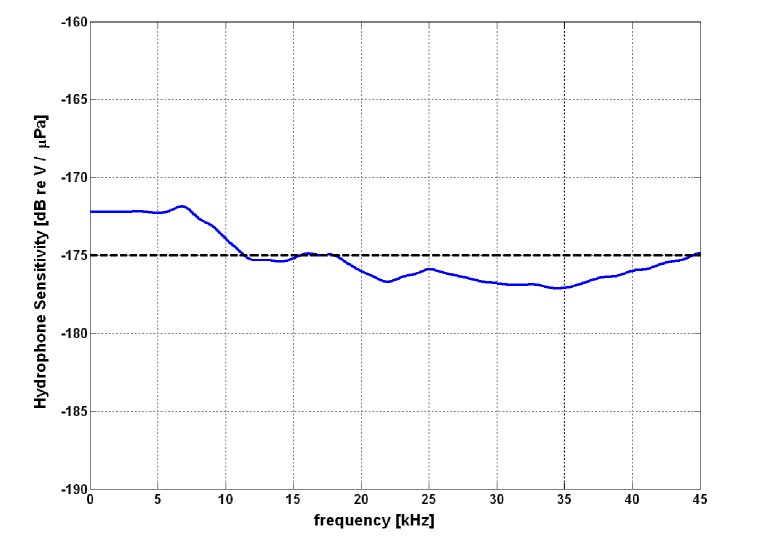
Figure 10: Hydrophone sensitivity (acoustic to electrical transduction factor) curve in units of dB re V/$\mu$Pa as a function of frequency provided by the hydrophone manufacturer for the hydrophone mounted in channel H3, the premplifier gain is 20 dB. The average value of -175 dB used to estimate the equivalent sound pressure density of electronic noise is shown in black, as a reference.

In Figure 11 is shown the sound pressure density of the acoustic noise in deep sea calculated for each month (blue curves), compared with the statistical error curve (black) as defined in the previous section. In Figure 12 is shown the average curve of sea acoustic noise SPD calculated over the whole data sample (blue line). The blue dashed curves take into account the error on the electronic noise power determination. The black dashed curves plotted in the same figure represent the sea noise sound pressure density expected in conditions of Sea State Zero (SS0) and Sea State Two (SS2) as defined by Urick Urick , i.e. the SPD of sea noise in conditions of absence of sea surface agitation (SS0), or low surface agitation (SS2) and absence of identifiable acoustic sources. A notable result for future underwater acoustic neutrino experiments is that the average acoustic sea noise in the band [$20\div 43$ kHz] amounts to $5.4\pm 2.2_{stat}\pm 0.3_{syst}$ mPa RMS (the systematic error is due to the uncertainty on the electronic noise power). This value is comparable to the estimated acoustic signature of a 10²⁰ eV neutrino interacting at 1 km distance from the detector (see reference Vandenbroucke2005 ).

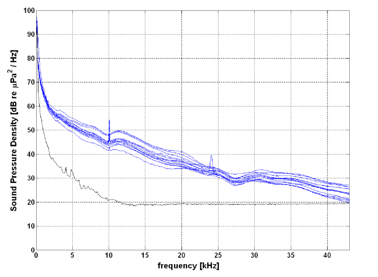
Figure 11: Sound pressure density curves of average sea acoustic noise as a function of month (blue). The black curve indicates the systematic error in the measurement due to the uncertainty on the electronic noise power spectrum.

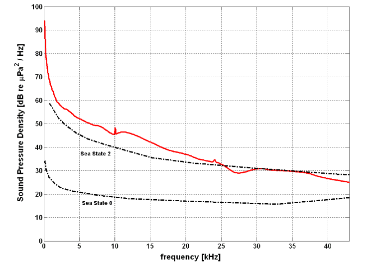
Figure 12: The blue solid line indicates the average sound pressure density of sea noise recorded with O$\nu$DE channel H3 from May 2005 to November 2006. The dashed blue lines indicate the systematic error on the average curve due to uncertainty of the electronic noise power spectrum. The black curves indicates respectively the expected SPD of the sea in conditions of Sea State 0 and Sea State 2 Urick .

7 Capability of acoustic sources tracking

Another characteristic of the station is the possibility to reconstruct the direction of detected acoustic sources. This is possible, in principle, since the antenna has a tetrahedral shape and the hydrophone signals are synchronised and phased offline. Nevertheless the hydrophone relative distances are about 1 m, therefore for distant sources (i.e. in far field condition) O$\nu$DE can only recover the angular direction of the source in the approximation of plane wavefront.

As an example, in figure 13 is shown the sperm whale click signal, quoted in figure 5, expanded in a different time-scale of 1000 samples (1/96 seconds). The signal is recorded first by H3 (installed on the frame apex) then by other hydrophones. Taking into account phase correction, due to phase shift introduced by the $f>1$ kHz hardware filter mounted on channels H2 and H4, the time delay between H3 and the other channels was recovered using a correlation function. Since the absolute position of hydrophones in the frame and the absolute orientation of the frame with respect to the sea bottom are known, the source angular direction was calculated minimizing the functional $G$($\vartheta$,$\varphi$), defined as:

$$G(\vartheta,\varphi)=\sum_{i=H1,H2,H4}[TDOA^{M}_{i,H3}(\vartheta,\varphi)-TDOA^{E}_{i,H3}(\vartheta,\varphi)]^{2}$$ (2)

where $TDOA^{M}$ is the measured time delay of the signal recorded by H3 with respect to the other hydrophones and $TDOA^{E}$ is the expected time delay between H3 and H1, H2, H4 for signal coming from a source located in the direction ($\vartheta$, $\varphi$). The results indicate that, in this case, the sperm whale was diving almost perpendicularly to the station ($\vartheta\simeq 87^{\circ}$) with a bearing of about 320^∘ with respect to North.

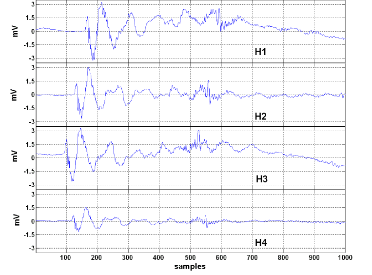
Figure 13: Click of a sperm whale recorded by the four hydrophones. The amplitude scale is in mV. Time Differences of Arrival (TDoA) between hydrophones are used to recover the whale angular position.

The estimate of angular direction reconstruction is affected by systematic errors due to the uncertainties in relative hydrophones distances (about 1 cm) and uncertainty in absolute frame orientation (see section 4.3). Preliminary results carried out with a known source operated from the sea surface indicate that this error is about $5^{\circ}$ both in $\vartheta$ and $\varphi$, assuming sound propagation in a homogeneous medium.

8 Interdisciplinary activities

The O$\nu$DE experiment other than providing long term data on the underwater noise, also provides a unique opportunity to study the acoustic emissions of marine mammals living in the area or transiting during their movements within the Mediterranean basin. The most notable result was about the sperm whale presence and transits in the area Science2007 . Several biological sounds, unknown sounds and many man-made noises (ship and fishboat noise, sonars, echosounders, airguns, and explosions) have been recorded and archived for reference. The collection of acoustic events collected so far represents a reference library to be used for discriminating/separating known sources from potential candidates of neutrino signatures in future larger dedicated arrays. Concerning whale detection, the most common sounds recorded are clicks produced by sperm whales arranged in regular sequences (inter-click interval in the range 0.5 s to 2 s), or in special patterned sequences (chirrups, codas, creaks) Pavan2000 . According to other studies in the Mediterranean Sea, sperm whales may dive to more than 1000 meters depth, but normally travel at 800$\div$1000 meters depth. Their source level is typically $200\div 220$ dB re 1 $\mu$Pa at 1 m on axis; the loudest clicks were received with sound pressure levels up to 170 dB re 1 $\mu$Pa Pavan2000 . Clicks were often recorded with high signal to noise ratio (SNR). Data from O$\nu$DE indicate a presence of sperm whales more consistent and frequent than previously believed. Although the transiting of sperm whales is known since the end of the XIX century Bolognari1949 , only a small few literature is available for the area. IFAW IFAW2003 reports a low sperm whale density in the Ionian basin with an average encounter of 5.8 whale groups for 1000 km of transect. With the O$\nu$DE station, in year 2005, sperm whales have been detected in 117 of the 231 (50.6%) recorded days. The analysis of 2006 data is still in progress but seems to confirm the 2005 data Pavan2008 .

9 Conclusions

The O$\nu$DE station successfully operated at the NEMO Test Site at 2000 m depth, 25 km offshore Catania (Sicily) from January 2005 to November 2006. Mechanical, electronics and data transmission and acquisition systems, designed and realised by INFN and CIBRA, demonstrated high reliability and fulfilled electronic noise design constraints. The station permitted for the first time a long term characterization of deep sea noise in the Mediterranean Sea in a large bandwidth ($0\div 43$ kHz), with optimal signal resolution. The electronics noise power spectrum of the detector was understood and evaluated to be $33\pm 0.3$ dB re 1 $\mu$Pa²/Hz above 5 kHz. It was also demonstrated that O$\nu$DE is capable to measure the sea noise Sound Pressure Density at the reference level of Sea State Zero.

Data analysis is presently addressed to characterize the underwater noise power level and its variations as a function of time. The analysis carried out so far shows that the average Sound Pressure Density of sea noise (over 13 months between May 2005 and November 2006) agrees with equivalent Sound Pressure Density of Sea State 2 for $f>25$ kHz. Larger values are recorded at lower frequencies due to better propagation of lower frequencies sound from surface to sea bottom and to man made noise (mainly ship traffic). The identification of different noise sources is on going.

The station also permits to localise noise sources using Time difference of Arrival of sound on the 4 hydrophones, in conditions of plane wave approximation for far field sources. The estimated error in the determination of the angular direction is about 5 degrees in azimuth and zenith angles.

The recorded data set was extensively used for interdisciplinary studies mainly addressed to search for cetaceans in the region; results indicated an unexpectedly large number of detections compared to previous studies.

10 Acknowledgements

The authors are grateful to L. Gualdesi and S. Buogo for help and suggestions, to L. Dedenko, S. Danaher, L. Thompson and M. Ardid for useful discussions. The authors also deeply thank the electronics workshop (head C. Calí) and the mechanical workshop (head B. Trovato) of LNS-INFN for their support in the construction of the experiment.

References

- (1) T. Gaisser, F. Halzen and T. Stanev, Phys. Rep. 258, 173 (1995).
- (2) K. Mannheim, Astron. and Astrophys 3, 295 (1995).
- (3) E. Waxmann and J. Bahcall, Phys. Rev. Lett. 78, 2292 (1997).
- (4) C. Distefano et al., Astrophys. J. 575, 378 (2002).
- (5) M.L. Costantini, F. Vissani, Astrophys. J. 23, 477 (2005).
- (6) M.A.Markov and I.M.Zheleznykh, Nucl. Phys. 27, 385 (1961).
- (7) M. Ackermann et al., Astrophys. J. 675, 1014 (2008).
- (8) J. Carr et al., Nucl. Instr. and Meth. A567, 428 (2006).
- (9) http://icecube.wisc.edu .
- (10) http://www.km3net.org .
- (11) E. Migneco et al., Nucl. Instr. and Meth. A567, 444 (2006).
- (12) G. Aggouras et al., Nucl. Instr. and Meth. A567, 452 (2006).
- (13) G. Pavan et al., J. Acoust. Soc. Am. 107, 6, 3487 (2000).
- (14) R.J. Urick, Sound Propagation in the Sea, Peninsula Publishing, ISBN 0-932146-08-2 (1982).
- (15) A. Achterberg et al., Phys. Rev. D76, 027101 (2007).
- (16) U. Katz, Nucl. Instr. and Meth. A567, 457 (2006).
- (17) G. Askarjan, Atomnaya Energia 3, 153 (1957).
- (18) J. Vandenbroucke, G. Gratta and N. Lehtinen, Astroph. Jour. 621, 301 (2005).
- (19) N.G. Lehtinen, Astrop. Phys. 17, 279 (2002).
- (20) P. Favali et al., Nucl. Inst. and Meth. A567, 2, 462 (2006).
- (21) P. Favali, L. Beranzoli Ann. Geophys. 49, 2-3, 705 (2006).
- (22) http://www.esonet-emso.org .
- (23) http://www.nautilus-gmbh.com .
- (24) http://www.reson.com .
- (25) http://www.cirrus.com .
- (26) http://www.aositilt.com .
- (27) http://www.rme-audio.com .
- (28) http://www.unipv.it/cibra .
- (29) http://www.matlab.com .
- (30) A. Bolognari, Bulletin de l’Institut Oc anographique 949, 1 (1949).
- (31) IFAW Report to ACCOBAMS Meeting of Parties, Palma de Mallorca, Spain (2004).
- (32) G. Pavan, G. Riccobene et al., in preparation.
- (33) Random Samples, Science 315, 5816, 1199 (2007).