Abstract

We investigate the utility of cosmological and astrophysical observations for distinguishing between supersymmetric theories. In particular we consider 276 pairs of models that give rise to nearly identical patterns of observables at hadron colliders. We focus attention on neutralino scattering experiments (direct detection of relic neutralinos) and observations of gamma-rays from relic neutralino annihilation (indirect detection experiments). Both classes of experiments planned for the near future will make measurements with exceptional precision. In principle, therefore, they will have the ability to be surprisingly effective at discriminating between candidate theories. However, the ability to distinguish between models will be highly dependent on future theoretical progress on such things as determination of the local halo density model and uncertainty in nuclear matrix elements associated with neutralino recoil events. If one imagines perfect knowledge of these theoretical inputs, then with extremely conservative physics assumptions and background estimates we find 101 of the 276 degenerate pairs can be distinguished. Using slightly more optimistic assumptions about background rates increases this number to 186 of the 276 pairs. We discuss the sensitivity of these results to additional assumptions made about nuclear matrix elements, the cosmological density of neutralinos and the galactic halo profile. We also comment on the complementarity of this study to recent work investigating these same pairs at a $\sqrt{s}=500~{}\mathrm{GeV}$ linear collider.

1 Introduction

With the first data from the Large Hadron Collider (LHC) rapidly approaching there is a shift in focus occurring in the theoretical community from how observations can be made to how observations can be used. That is, assuming physics beyond the Standard Model (BSM) is discovered in the early stages of LHC data collection, how can the large set of measurements that will eventually be made be used to reconstruct the Lagrangian of the underlying physics model? There are many approaches to answering this question. The direct approach assumes a rough ansatz for the BSM physics can be postulated early on, and then mass eigenstate information can be extracted by reconstructing specific decay chains within this model framework [1]. Another, more top-down approach is to perform direct fits to certain theoretically motivated models which are presumed to be defined with a relatively small number of input parameters [2]. Recently, several groups have begun working on hybrid approaches that combine bottom-up exclusive measurements with top-down global analyses, such as the construction of on-shell effective theories [3] or the identification of mass hierarchy patterns [4]. The possible redundancy of these techniques is a welcome cross-check, and all are likely to be of utility in the early stages of LHC data-taking. This process of reconstructing both the form and the parameters of the underlying new physics Lagrangian is commonly referred to as “inverting” the LHC data.

An obvious question to ask is whether this reconstruction procedure will yield a unique solution. The answer is likely to be yes if a relatively simple and well-constrained theory gives a good fit to the data [5]. But for even slightly more complicated theories the answer becomes ambiguous. Recently, Arkani-Hamed et al. [6] studied the minimal supersymmetric standard model (MSSM), with 15 free parameters used to determine the resulting spectrum and phenomenology. The authors found that it is highly probable (perhaps inevitable) that even after hundreds of measurements – consisting of counting events with distinct final-state topologies as well as examining the shapes of a wide range of kinematic distributions – more than one set of these 15 parameters will be a good fit to the data. In fact, a set of parameters which fit the data may well have several such “degenerate twins” in the parameter space of the theory. The challenge of disentangling these degenerate pairs is the LHC Inverse Problem.

While the conclusion of [6] is sobering, it might not seem especially surprising. Within a model system as complex as the MSSM it is possible to engineer two theories with similar collider signatures because some aspects of the model (such as the wavefunction of the lightest stable neutralino, or the value of the parameter $\tan\beta$) are not easily probed in a hadron collider. While it is very difficult to construct a degenerate twin for any particular supersymmetric model, given enough sampling of the parameter space it is not difficult to find pairs of points that are degenerate to within the experimental error desired. For example, over 43,000 parameter points were considered in [6], yielding 283 degenerate pairs of parameter sets. Degeneracy here was measured with respect to 1808 observations in 10 fb^-1 of LHC data, after crude cuts were made to reduce the Standard Model backgrounds. One can argue about how many of these 283 pairs of models could, in fact, be distinguished if only the authors had used a different set of observations, or considered more integrated luminosity, or used more exclusive techniques such as decay-chain reconstruction in the analysis. Undoubtedly many of these pairs would indeed be distinguished, eventually, at the LHC. Additional research in each of these directions (using the degenerate pairs of [6] as a guide) is warranted.

In this letter we choose to take the primary conclusion of [6] at face value. Thus we will assume that (R-parity conserving) supersymmetry is discovered early at the LHC. Yet we also assume that even as LHC data accumulates isolated parameter sets for the MSSM emerge which cannot be distinguished with LHC data alone. We will use the 283 degenerate pairs of [6] as proxies for these post-LHC degeneracies. Here we will investigate the efficacy of cosmological and astrophysical observations associated with the stable relic neutralino in distinguishing between these pairs. We believe this to be a particularly fruitful area to study. The conspiracy of soft supersymmetry breaking parameters necessary for two models to give similar signatures at the LHC often gave rise to spectra of gauginos with common mass differences. The wave-functions of these mass eigenstates, however, were often dramatically different between the two degenerate models. Unfortunately, the wave-function composition of the lightest neutralino (usually the lightest supersymmetric particle, or LSP) is particularly difficult to measure at the LHC. On the other hand, it is well known to have dramatic effects on the cosmology of this stable LSP – both in its thermal relic abundance [7] and on the prospects for its experimental detection at dark matter related experiments [8].

The present work is very much in the spirit of (and complementary to) recent work [9] in which these same pairs were studied at a $\sqrt{s}=500~{}\mathrm{GeV}$ international linear collider (ILC). The results of that study were mixed. When charged superpartners were kinematically accessible they were (more often than not) also detectable above the Standard Model background. When only neutral superpartners were kinematically accessible that was not true. When one or both of the degenerate models in a pair had an accessible and visible charged superpartner they were generally distinguishable at a 500 GeV linear collider. Unfortunately only 57 pairs met this criterion with a $5\sigma$ level of distinguishability (the number becomes only 63 when the criterion is relaxed to the $3\sigma$ level). At issue is the relatively high mass of low-lying gaugino states in the degenerate pair sample of [6]. The authors of [9] conclude that a center-of-mass energy of $\sqrt{s}=1~{}\mathrm{TeV}$ would fare much better at distinguishing between these pairs. But given the uncertainties currently surrounding the fate of any international linear collider effort, it seems prudent to ask whether additional information from outside the collider arena can profitably be brought to bear on the issue of breaking degeneracies within the allowed supersymmetric parameter space.

To that end, we will introduce the degenerate model pairs in Section 2, briefly discussing the methodology of Arkani-Hamed et al. in Section 2.1. A discussion of our analysis of these pairs begins in Section 2.2 with a look at some of the global properties of this model set. We will find that almost all of the models predict a thermal relic abundance outside a 95% confidence level region about the preferred value deduced from observations of the cosmic microwave background by the WMAP experiment. This is not a surprise since none were designed to meet this constraint (or indeed several other indirect constraints on supersymmetric models). This observation leads to a natural classification of the models into those which are at least consistent with all indirect constraints, and those which are at odds with at least one such constraint. We will use this classification as a guide to present our subsequent results. In Section 3 we discuss the ability of direct detection experiments to distinguish models, and in Section 4 we discuss the same for indirect detection experiments that look for photons from relic neutralino annihilation. The net effect of all of these experiments in differentiating between the degenerate models is presented in the concluding section.

One final comment is in order before we begin. By “distinguishable” we here mean that any two predicted signals – such as the number of observed nuclear recoils in a direct detection experiment – could be distinguished from one another with a high degree of statistical significance. When theoretical uncertainties are neglected the previous sentence becomes a statement about the inherent resolving power of a particular experiment (or experiments). For example, this is what is typically meant by the concept of distinguishing between models in studies that focus on collider signals. But the dark matter arena is in many ways more difficult than studying signatures at the LHC or ILC: rather than studying similar detectors at a single facility with a well-modeled background (and high event rates) we must here work with a large variety of experimental configurations. Event rates are generally low and background estimations less well understood than in the collider environment. Finally, it is generally the case that theoretical inputs, such as the assumed dark matter halo profile or the value of certain nuclear matrix elements, are often the largest sources of uncertainty. Statements about distinguishing candidate theories must always be understood within this context. Because of these uncertainties separating two post-LHC candidate models will be difficult without the assistance of having a detailed astrophysical model as well as a concrete particle physics model (or in this case, a pair of models) at hand. This point has been emphasized recently in [10]. Therefore, in this paper we will generally make statements in which a fixed astrophysics model (such as a particular galactic halo profile) is assumed, as is common in the literature. “Distinguishability” under these assumptions then essentially reduces to a consistency check between one of a pair of models suggested by the LHC data and an assumed dark matter signal. Within this framework we make every effort to be as conservative as possible and present our results under a variety of assumptions so that the reader can make his or her own comparisons. We will return to the issue of theoretical uncertainties and the broader notion of separating models throughout this work, and make comments on how they might be potentially resolved in the conclusion.

2 The Degenerate Pairs

2.1 Summary of Arkani-Hamed et al.

In this subsection we give a very brief summary of the methodology of Arkani-Hamed et al. [6], which serves as a way of introducing the degenerate model pairs. As mentioned in the introduction, the theory considered was that of the MSSM, with 15 parameters used to define the spectrum and interactions

$$\left\{\begin{array}[]{c}\tan\beta,\,\,\mu,\,\,M_{1},\,\,M_{2},\,\,M_{3}\\ m_{Q_{1,2}},\,m_{U_{1,2}},\,m_{D_{1,2}},\,m_{L_{1,2}},\,m_{E_{1,2}}\\ m_{Q_{3}},\,m_{U_{3}},\,m_{D_{3}},\,m_{L_{3}},\,m_{E_{3}}\end{array}\right\}\,.$$ (1)

Here $\tan\beta$ is the ratio of the two scalar Higgs vevs, $\mu$ is the supersymmetric Higgsino mass parameter and $M_{i}$ represent the soft supersymmetry breaking masses of the gauginos. Note that all three gaugino masses are independent here, allowing for a wide array of predictions in the dark matter arena. In the next two lines of (1) $m_{X_{1,2}}$ is the soft supersymmetry breaking mass of the first two generations of the scalar field $X$, taken to be identical, while $m_{X_{3}}$ is soft mass for the third generation of field $X$. We will refer to any such set of 15 values for the quantities in (1) as a “model.” Other parameters required to establish the spectrum were taken as fixed, and thus are the same for all models considered: the pseudoscalar Higgs mass at $m_{A}=850~{}\mathrm{GeV}$ and the scalar trilinear couplings at $A=800~{}\mathrm{GeV}$ for third generation squarks and $A=0$ for the sleptons. These are parameters valid at the electroweak scale, so no renormalization group evolution is required. Constraints were placed on the sizes of some parameters in order to make the collider simulation tractable.

Over 43,000 parameter sets were chosen at random and 10 fb^-1 of LHC data was generated for each such model – a massive computational undertaking. Data was simulated using PYTHIA [11] and the detector response was modeled using the PGS detector simulator [12]. A set of initial cuts were used to simulate what would be required in a true analysis to reduce the Standard Model background, though no actual Standard Model processes were included in the analysis itself. This analysis had two components. The first counted the number of events which had one of a number of suitably defined final state topologies. The second component included studying the shapes of a number of key kinematic distributions of final state decay products. These shapes were parameterized by taking the relevant histogram and binning the data into even numbers of quantiles, then recording the position of the quantile boundaries. In this way both components of the data analysis could be included in a $\chi^{2}$-like variable. In total there were 1808 such quantities $s_{i}$ for each model, the set of all 1808 being called the “signature” of the model at the LHC.

These individual $s_{i}$ values were grouped together into a variable similar to a traditional chi-squared quantity,

$$(\Delta\,S_{AB})^{2}=\frac{1}{N_{\rm sig}}\sum_{i}\left(\frac{s_{i}^{A}-s_{i}^{B}}{\sigma_{i}^{AB}}\right)^{2}\,,$$ (2)

where $A$ and $B$ represent two different models, $N_{\rm sig}$ is the total number of signatures considered and $\sigma_{i}^{AB}$ is a measure of the error associated with the $i$-th signature

$$\sigma_{i}^{AB}=\sqrt{(\delta s_{i}^{A})^{2}+(\delta s_{i}^{B})^{2}+\left(f_{i}\frac{s_{i}^{A}+s_{i}^{B}}{2}\right)^{2}}\,.$$ (3)

The final quantity is meant to represent the error associated with incomplete removal of Standard Model background events from the data sample. The value $f_{i}=0.01$ was chosen for all observables except for the total event rate, for which $f_{i}=0.15$ was chosen. The quantity (2) therefore provides a reasonable metric for measuring distances in signature space. The next question is how far apart two models need to be in this space to be deemed “distinguishable.” There are a number of reasonable answers. The criterion chosen in [6] is as follows. Imagine taking any supersymmetric theory and performing a collider simulation. Now choose a new random number seed and repeat the simulation. Due to random fluctuations we expect that even the same set of input parameters, after simulation and event reconstruction, will produce a slightly different set of signatures. Now repeat the simulation a large number of times, each with a different random number seed. Use (2) to compute the distance of each new “model” with the original simulation. While we might expect the distribution of $(\Delta S_{AB})^{2}$ to be narrow with a central value near zero, we nevertheless expect there to be some spread. Find the value of $(\Delta S_{AB})^{2}$ which represents the 95th percentile of the distribution. This might be taken as a measure of the uncertainty in “distance” measurements associated with statistical fluctuations. In [6] this number was determined to be $(\Delta S_{AB})^{2}\big{|}_{\rm 95th}=0.285$. Any two genuinely different models for which the calculated $(\Delta S_{AB})^{2}$ is less than 0.285 were therefore considered to be degenerate with each other.

Applying this criterion, Arkani-Hamed et al. found 283 pairs of models which failed to be distinguished at the LHC in their study (albeit with only 10 fb^-1 of data). As many models were degenerate with more than one other set of parameters, the total number of unique individual parameter sets represented in this sample was 384, from an original set of over 43,000 models. We were generously provided with the values of the parameters in (1) for these 384 models from the collaboration in [6]. We used these input parameters to generate 50,000 events for each model at the LHC, roughly equivalent to 5 fb^-1 of data, using the same combination of PYTHIA + PGS. While a complete reproduction of the analysis in that work would beyond the scope of our study, we did use the variables defined in (2) and (3) to examine a reduced set of 36 signatures in the generated data. We confirmed that the 283 model pairs were highly degenerate at the LHC, most falling well within our threshold $(\Delta S_{AB})^{2}\big{|}_{\rm 95th}=0.63$ for indistinguishability.

2.2 Classification and further constraints

Before proceeding to a study of dark matter observations, we wish to consider a few global aspects of this model set. In studying the signatures of these models at a future linear collider the authors of [9] encountered an initial problem: PYTHIA computes physical gaugino masses only at the tree-level. Many of the models in this set have soft supersymmetry breaking gaugino masses such that the lightest chargino is slightly less massive than the lightest neutralino. This is normally not a disaster as loop corrections to the mass eigenstates remedy the problem. In PYTHIA, however, the problem is instead rectified by artificially adjusting the chargino mass to be the mass of the lightest neutralino plus twice the neutral pion mass. In PYTHIA 6.4 this comes with a warning flag. In our analysis 149 of the 384 models were so flagged. A similar number of problematic models were observed in [9]. In studying the linear collider signatures of these models the mass difference between these two states is a crucial parameter in determining the detectability of the low-lying chargino state. Without a reliable calculation of this mass difference the authors of [9] decided to jettison these models. In our case the mass difference is crucial only in the determination of the relic neutralino density, $\Omega_{\chi}{\rm h}^{2}$, since the rate of neutralino-chargino coannihilation in the early universe is very sensitive to this quantity.

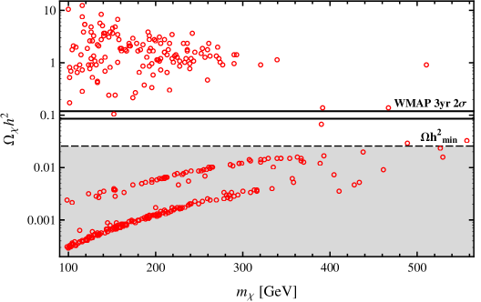
Figure 1: Thermal relic abundance of neutralino LSP for 378 models from [6]. Prediction for the thermal relic abundance $\Omega_{\chi}{\rm h}^{2}$, as computed by DarkSUSY, is displayed as a function of the LSP mass $m_{\chi}$. The $2\sigma$ band in this quantity favored by the WMAP three-year data set is indicated by the solid horizontal lines. The shaded region bounded by the dashed line represents the set of models for which the local number density of neutralinos should be rescaled.

We compute this relic density using the software package DarkSUSY [13] which includes the most significant one-loop corrections to the neutralino mass matrix, eliminating the problem with the chargino/neutralino mass difference. We will discuss the results of that computation below. Here we merely point out that the cosmological density represented by the number $\Omega_{\chi}{\rm h}^{2}$ is not directly related to any of the observables we will be using to distinguish between models. Instead it is the local halo density that is relevant and the relationship between the two quantities is not a precise one. We will therefore keep all 149 of these model points in our analysis that follows. However, for six models the DarkSUSY spectrum calculation returned a stau as the lightest supersymmetric particle (LSP), which is certainly a problem for computing cosmological observables. We will eliminate all six of these models from our study, leaving us with 378 models comprising 276 degenerate pairs. The distribution of thermal relic neutralino abundances for these 378 models is shown in Figure 1 as a function of the mass of the lightest neutralino. The narrow band indicated by the solid horizontal lines is the $2\sigma$ region favored by the WMAP three-year data [14]

$$0.0855<\Omega_{\chi}{\rm h}^{2}<0.1189\,.$$ (4)

All but one of the 378 models lie outside the band of values favored by the WMAP data; 145 exceed the upper bound while 232 fall below the lower value. Of the latter, 224 have $\Omega_{\chi}{\rm h}^{2}\leq 0.025$ (indicated by the dashed line in Figure 1). This value is used as a crude measure of the point at which the relic particle in question can no longer account adequately for the local halo density of our galaxy [15]. We will return to this issue in a moment.

The implication of Figure 1 is that there are no pairs among the 276 for which both models in the pair give a relic abundance within the range of (4). This should not be interpreted to mean that degenerate pairs do not exist which are fully consistent with this range – nor that such degenerate pairs are in particularly obscure parts of the supersymmetric parameter space. It means nothing more than that the conventional top-down method of searching for such pairs is horribly inefficient. The authors of [6] were interested in general issues of LHC phenomenology for which the value of $\Omega_{\chi}{\rm h}^{2}$ is wholly irrelevant. In fact, restricting their attention only to models which satisfy (4) would have unduly biased their study. The ultimate relic density of neutralinos can be a very sensitive function of the masses and mixings of the superpartner spectrum. We have no doubt that many of these model pairs could be adjusted to give degenerate results at the LHC while providing for a reasonable value of $\Omega_{\chi}{\rm h}^{2}$. Therefore we will analyze the dark matter related signatures for all 378 model points in what follows. Nevertheless we will group those which exceed the upper limit in (4) separately, as it is generally quite difficult to engineer processes in the early universe to reduce the thermal abundance of a stable relic [16]. By contrast, it is not hard to imagine ways to enhance the relic abundance of a stable neutralino through non-thermal mechanisms [17]. For that reason we will not eliminate models for which $\Omega_{\chi}{\rm h}^{2}$ is below the lower bound of (4) or consider them unphysical. However, when calculating observable quantities that depend on the relic neutralino number density $n_{\chi}$ present in our galaxy (or the energy density $\rho_{\chi}=m_{\chi}n_{\chi}$) we will rescale the assumed local density of $(\rho_{\chi})_{0}=0.3$ GeV/cm³ by the multiplicative factor $r_{\chi}={\rm Min}(1,\,\Omega_{\chi}{\rm h}^{2}/0.025)$.

In [6] the authors were careful to ensure that all direct search bounds for superpartners were satisfied by the resulting spectrum. They were less concerned with the bound on the lightest CP-even Higgs mass from LEP, nor with other indirect constraints on supersymmetry. Consider, for example, the following bounds taken from [18]

$$\begin{array}[]{c}m_{h}\geq 114.4~{}\mathrm{GeV}\\ 2.65\times 10^{-4}\leq{\rm Br}(B\to X_{s}\gamma)\leq 4.45\times 10^{-4}\\ \frac{g_{\mu}-2}{2}\big{|}_{\rm SUSY}\leq 4.7\times 10^{-9}\end{array}$$ (5)

for the mass of the lightest CP-even Higgs, branching fraction for $b\to s\gamma$ events, and the supersymmetry contribution to the anomalous magnetic moment of the muon, respectively. These bounds were violated by 43, 101 and 6 models, respectively, from the set of 378. All of these have marginal relevance to the physics of the LHC, and even less relevance to the physics we discuss in this paper. Nevertheless, we will designate a subset of the 378 models as “physical” if they have a relic density below the upper bound in (4) and satisfy all three constraints (5). There are then 127 such “physical” models, arranged in 77 indistinguishable pairs. Throughout the subsequent work we will focus on this physical subset where appropriate.

	Models	Pairs
Initial Set	378	276
PYTHIA chargino warnings	149	124
Relic Density
$\Omega_{\chi}{\rm h}^{2}>0.1189$	145	116
$\Omega_{\chi}{\rm h}^{2}<0.0250$	224	164
Additional Constraints
$m_{h}<114.4$ GeV	43	52
${\rm Br}(B\to X_{s}\gamma)>4.45\times 10^{-4}$	101	98
$a_{\mu}\big{|}_{\rm SUSY}>4.7\times 10^{-9}$	6	6
Visible at 500 GeV ILC	190	173
Remove PYTHIA chargino warnings	68	65
All Physical Conditions Satisfied	127	77

Table 1: Summary of global properties of the 378 models. Statistics listed under the heading “Models” give the number of individual model points satisfying the stated property. Statistics in the column labeled “Pairs” count the number of pairs where at least one of the two models in the pair satisfies the stated property. If a model has $\Omega_{\chi}{\rm h}^{2}<0.1189$ and fails none of the tests listed in the Additional Constraints section it is counted in the last row of the table. If both models in a pair do so, the pair is counted in the last row.

Finally, it is useful to consider how dark matter based observations can buttress the results of [9]. While we do not know precisely which of the 276 pairs were deemed to be distinguishable at a $\sqrt{s}=500~{}\mathrm{GeV}$ linear collider, we can estimate which models would be visible at such a machine by simply requiring that a chargino or charged slepton be kinematically accessible. To be conservative we require a mass less than $240~{}\mathrm{GeV}$ to be deemed kinematically accessible. With this assumption we estimate that 190 models would be visible at a 500 GeV linear collider; or only 68 models if we reject those generating a chargino mass warning flag in PYTHIA. This is to be compared with 63 model pairs that were found to be distinguishable at $3\sigma$ in [9], where at least one model was accessible and detectable. We will comment on this subdivision of the 378 models in the conclusion section of this work. A summary of the various classifications introduced in this section is given in Table 1.

3 Direct Detection Experiments

Before taking our first look at potential experimental data let us recall the assumptions underlying our thought experiment. We imagine that LHC data equivalent to several years running has been accumulated and analyzed. This analysis has been restricted to broadly inclusive observables of the sort considered by Arkani-Hamed et al. – that is, we do not allow ourselves knowledge of the mass of individual mass eigenstates. Undoubtedly such information will become available through the study of isolated decay chains and kinematic end-point variables associated with them. But to be true to the spirit of “model-independence” of [6] we do not allow any such knowledge in what follows. This is particularly relevant in the case of the mass of the lightest supersymmetric particle, upon which many observable quantities we will consider depend. We will comment further on the power of this information in the concluding section of this paper.

However we do imagine that some sort of global fit has been performed, in which the values of these inclusive signatures have been calculated as a function of a sufficiently broad parameter space within the MSSM. At the end of this process two parameter sets of the form of (1) (i.e. two “models”) have emerged as equally good fits to the observed data. From this perspective our 276 degenerate model pairs represent 276 different possible outcomes of this global fitting process. We therefore have two candidate parameter sets “A” and “B” from which we can calculate the theoretical expectation for various dark matter observables $s_{i}$ for both models in the pair. To claim that a particular experiment has the power to distinguish between models A and B we require two properties simultaneously. First, the values of $s_{i}^{A}$ and $s_{i}^{B}$ need to be large enough that both are detectable above the relevant background for the experiment in question. Second, the values of $s_{i}^{A}$ and $s_{i}^{B}$ need to be sufficiently separated to give a statistically significant difference when measured with respect to the appropriate mutual error $\sigma_{i}^{AB}$. It is possible to relax the first assumption by requiring only that one of the two experiments yield a detectable signal $s_{i}$, which can be distinguished statistically from $s_{i}=0$. This was the approach taken in [9]. But given the inherent uncertainties, both experimental and theoretical, associated with dark matter observables we prefer a more conservative requirement for distinguishability.

With this in mind we will focus in this section on direct detection of relic neutralinos via their scattering from target nuclei. Scattering events are signaled by the detection of the nuclear recoil for elastic scatters, or by detecting the resulting ionization of the target nucleus for inelastic scattering [20]. We consider a range of current and future experiments listed in Table 2. For each experiment we give the target nucleus, the target mass and the physics object (or objects) which are actually detected to signal a scattering event. The first three experiments in Table 2 are currently taking data and setting limits on nucleon-neutralino interaction cross sections. The target mass for these experiments represents the true fiducial mass. The remaining experiments are in various stages of development and planning. The entry in the target mass column is only a nominal mass – the actual fiducial mass used for data taking is typically smaller by a significant factor.

Ref.	Experiment Name	Target	Mass (kg)	Detected Object(s)
[23]	CDMS II	Ge	3.75	athermal phonons, ionization charge
[24]	XENON10	Xe	5.4	scintillation photons, ionization charge
[25]	ZEPLIN II	Xe	7.2	scintillation photons, ionization charge
[26]	SuperCDMS (Soudan)	Ge	7.5	see CDMS II
[26]	SuperCDMS (SNOlab)	Ge	27	see CDMS II
[26]	SuperCDMS (DUSEL)	Ge	1140	see CDMS II
[27]	EDELWEISS-2	Ge	9	athermal phonons, ionization charge
[28]	XENON100	Xe	170	see XENON10
[28]	XENON1T	Xe	1000	see XENON10
[29]	LUX	Xe	350	scintillation photons, ionization charge
[30]	ZEPLIN III	Xe	8	see ZEPLIN II
[30]	ZEPLIN IV	Xe	1000	see ZEPLIN II

Table 2: List of direct detection experiments considered. The first three experiments listed (CDMS II, XENON10 and ZEPLIN II) are currently taking data and have recently reported limits on neutralino-nucleus interaction rates. The masses for these three experiments are their respective reported fiducial masses. All other experiments listed are projected for some time in the future and the masses given are nominal mass values.

A couple of statements about this list are in order. These are not all the experiments that one might consider, even if one restricts attention to solely those based on germanium or xenon. The choice here reflects the desire for simplicity of presentation and reliability of background estimations. There are essentially two classes of detector here: cryogenic germanium bolometers and dual-phase liquid/gas xenon detectors. Both types are currently operational in at least one experiment and producing results. Both detector technologies have been shown to be scalable and significantly larger installations of each technology are planned (the nine experiments below the double line in Table 2). By taking measured background rates in current experiments it is possible to extrapolate reliably to the large scale experiments imagined in the future. Furthermore, by focusing on two target materials it is possible to present the reach and resolving power of multiple experiments in terms of just two quantities: exposure time in germanium or xenon. This provides a desirable degree of simplicity in presenting the results that follow.

To compute the interaction rate of relic neutralinos with the nuclei of the target material one considers both spin-dependent (SD) and spin-independent (SI) interactions. For target nuclei with large atomic numbers the SI interaction, which is coherent across all of the nucleons in the nucleus, tends to dominate. This is true of xenon and, to a slightly lesser extent, germanium as well. The SI cross section $\sigma^{\mathrm{SI}}$ is computed in DarkSUSY on an arbitrary nuclear target via [13]

$$\sigma^{\mathrm{SI}}_{\chi i}=\frac{\mu^{2}_{i\chi}}{\pi}\big{|}ZG^{p}_{s}+(A-Z)G^{n}_{s}\big{|}^{2}\,,$$ (6)

where $i$ labels the nuclear species in the detector with nuclear mass $M_{i}$, $\mu_{i\chi}$ is the reduced mass of the nucleus/neutralino system $\mu_{i\chi}=m_{\chi}M_{i}/(m_{\chi}+M_{i})$, and $A$ and $Z$ are the target nucleus mass number and atomic number, respectively. The quantities $G^{p}_{s}$ and $G^{n}_{s}$ represent scalar four-fermion couplings of the neutralino to point-like protons and neutrons. They can be described schematically as

$$G^{N}_{s}=\sum_{q=u,d,s,c,b,t}\langle N|\bar{q}q|N\rangle\times\left({\rm SUSY\,\,parameters}\right)\,,$$ (7)

where the quantity in parenthesis is calculable once the details of the supersymmetric model are specified. The initial nuclear matrix elements, however, are at present not calculable from first principles. Their values must be inferred from pion-nucleon scattering data. Depending on the methodology employed in this analysis, different values for this important set of parameters can be extracted – particularly for the case of the $\pi\,N$ $\Sigma$-term [31]. The importance of the resulting uncertainty in this parameter on predictions for dark matter interaction cross-sections was recently considered in [32, 33], where it was shown to be potentially quite large. We will return to this issue at the very end of this section. For what follows we will simply use the default values in DarkSUSY for all nuclear matrix elements.

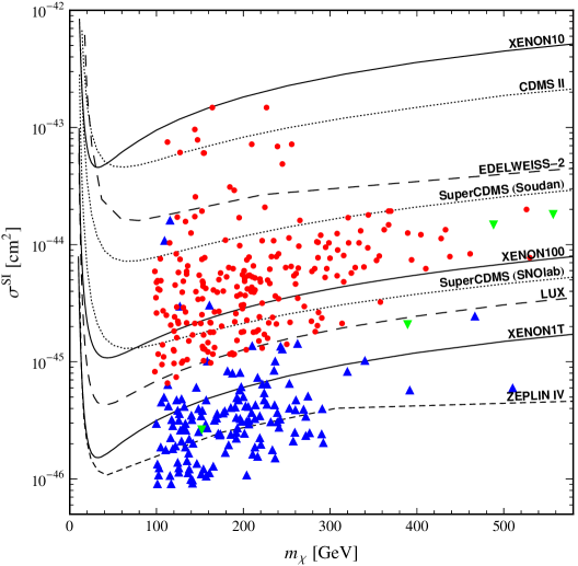
Figure 2: Spin independent neutralino-proton interaction cross-section as a function of $m_{\chi}$ for the 378 models. The 378 models are divided into three groupings: those with $\Omega_{\chi}{\rm h}^{2}>0.1189$ (darker filled triangles), $0.025<\Omega_{\chi}{\rm h}^{2}<0.1189$ (lighter inverted triangles) and $\Omega_{\chi}{\rm h}^{2}<0.025$ (filled circles). Sensitivity curves for several of the experiments in Table 2 are overlaid on the plot. These curves were taken from the web-based utility [21].

It is common in the literature to graphically exhibit the reach of any given experiment in terms of a variable in which results can be compared easily. This lingua franca is $\sigma^{\mathrm{SI}}_{\chi p}$ – the interaction cross section of the neutralino with the target nucleus, normalized to an equivalent interaction cross section on protons [22]. In Figure 2 we therefore plot all 378 models in the $(m_{\chi}\,,\sigma^{\mathrm{SI}}_{\chi p})$ plane. The points in Figure 2 are separated into those for which $\Omega_{\chi}{\rm h}^{2}>0.1189$ (darker filled triangles), $0.025<\Omega_{\chi}{\rm h}^{2}<0.1189$ (lighter inverted triangles) and $\Omega_{\chi}{\rm h}^{2}<0.025$ (filled circles). The nominal reach for a selection of the experiments in Table 2 is also given, indicated by the various lines as labeled in the figure. For the XENON10 and CDMS II experiment these lines represent actual exclusion curves. The limits arising from the ZEPLIN II data are weaker (on the order of $10^{-42}$ cm²) and therefore do not appear on the figure.

At first glance Figure 2 seems to indicate that several of the models should have already given a discernable signal in one or more current direct detection experiments. We would like to argue that Figure 2 is somewhat deceptive in this regard. Plots similar to Figure 2 are typical in the high energy physics literature. They are sufficient for a crude analysis of whether a particular experiment has the sensitivity to “discover” or exclude a particular model in question. But such a plot fails to adequately describe the challenge of distinguishing two candidate theories. Experiments measure counting rates, not cross sections. The relation between the two involves additional assumptions about the local density of relic neutralinos and their velocity distribution. As mentioned in Section 2.2 nearly 60% of the models we are studying have $\Omega_{\chi}{\rm h}^{2}\leq 0.025$ – including all of the models whose cross sections are nominally above the XENON10 and CDMS II reach curves in Figure 2. The experimentally measured quantity – the rate of nuclear recoils – involves the product of the spin-independent cross section and the neutralino number density $n_{\chi}$. If we rescale this number density by $r_{\chi}={\rm Min}(1,\,\Omega_{\chi}{\rm h}^{2}/0.025)$ we find that none of the 378 models would yield more than one or two events in either experiment in the reported exposure time accumulated thus far. This exemplifies the importance of working directly with count rates, as well as the importance of knowing the background rate for these experiments.

An estimate of the rate of neutralino-nucleon scattering events (in units of events/kg/day) can be computed from (6) according to

$$R\sim\sum_{i}\Phi_{\chi}\frac{\sigma^{\mathrm{SI}}_{\chi i}}{M_{i}}=\sum_{i}\frac{\langle v_{\chi}\rangle\rho_{\chi}\sigma^{\mathrm{SI}}_{\chi i}}{m_{\chi}M_{i}}\,,$$ (8)

where $\Phi_{\chi}$ is the average neutralino flux through the detector and $\langle v_{\chi}\rangle$ is the average speed of the neutralino relative to the target [15]. For the sake of a quick estimate one can take this velocity to be $\langle v_{\chi}\rangle$ = 270 km/s.

For our rate calculations we use a more precise formulation that takes into account the nature of the target. We begin by using DarkSUSY to compute the differential rate of interactions per unit recoil energy via [15]

$$\frac{dR}{dE}=\sum_{i}c_{i}\frac{\rho_{\chi}\sigma_{\chi i}|F_{i}(q_{i})|^{2}}{2m_{\chi}\mu^{2}_{i\chi}}\int_{v_{min}}^{\infty}\frac{f(\vec{v},t)}{v}d^{3}v\,.$$ (9)

Now we sum over all nuclear species present, with $c_{i}$ being the mass fraction of species $i$ in the detector. The quantity $f(\vec{v},t)\,d^{3}v$ is the neutralino velocity distribution (presumed to be Maxwellian) with $v=|\vec{v}|$ the neutralino velocity relative to the detector. Finally $|F_{i}(q_{i})|^{2}$ is the nuclear form factor for species $i$, with $q_{i}=\sqrt{2M_{i}E}$ being the momentum transfer for a nuclear recoil with energy $E$. For the purpose of this analysis we will use the output differential rates from DarkSUSY, calculated via (9), over a range of recoil energies relevant to the desired experiment. For a given experiment there is typically a minimum resolvable recoil energy $E_{\rm min}$ as well as a maximum recoil energy $E_{\rm max}$ that is considered. These energies are $\mathcal{O}(10-100)$ keV and represent the nuclear recoil energy of (9) inferred from the observed energy of the detected physics objects. The range of integration is generally different for each experiment and is determined by the physics of the detector as well as the desire to maximize signal significance over background. For example, the first three (active) experiments in Table 2 integrate over the ranges

$${\rm CDMS\,\,II} : 10\,{\rm keV}\leq E_{\rm recoil}\leq 100\,{\rm keV}$$

$${\rm XENON10} : 4.5\,{\rm keV}\leq E_{\rm recoil}\leq 26.9\,{\rm keV}$$

$${\rm ZEPLIN\,\,II} : 14\,{\rm keV}\leq E_{\rm recoil}\leq 56\,{\rm keV}\,.$$ (10)

We perform a numerical integration of (9) by constructing an interpolating function for the differential rate sampled in $0.5$ keV intervals. Given the wide variety of integration ranges exemplified by (10), and in order to make meaningful comparisons across different experiments (including the many experiments in Table 2 that are still in the planning stages), we perform the integration using two possible energy ranges

$$R_{1} : 5\,{\rm keV}\leq E_{\rm recoil}\leq 25\,{\rm keV}$$

$$R_{2} : 10\,{\rm keV}\leq E_{\rm recoil}\leq 100\,{\rm keV}\,.$$ (11)

The rate $R_{1}$ would cover the region that appears to be typical of the dual-phase xenon detectors, while the larger range for the rate $R_{2}$ seems to be typical for the germanium-based bolometer experiments. Empirically we find that the rate integrated over $R_{2}$ is roughly twice that integrated over $R_{1}$:

$$R^{\rm Xe}_{2}=1.86\,R^{\rm Xe}_{1}\quad\quad\&\quad\quad R^{\rm Ge}_{2}=2.24\,R^{\rm Ge}_{1}\,.$$ (12)

Finally, to reverse-engineer the reach curves we must have some notion of how well a particular experiment can distinguish nuclear recoils due to neutralino scattering from fakes and background events. This is also relevant to the question of whether two possible signals can reliably be distinguished at any given experiment. All of the experiments in Table 2 collect charge as part of the detection process, and it is this ionization charge that plays an important role in background discrimination. Therefore background sources are quite similar across the various types of experiments. We can break these backgrounds into two crude classes: “true” neutron recoils and “fake” neutron recoils. In the former case we are thinking of nuclear recoils that are measured in the detector but which did not originate from a passing neutralino. They are generally the result of neutrons produced in one of two ways: alpha-decays originating in the material making up (or surrounding) the experimental chamber or neutron recoils induced from cosmic-ray muons penetrating the experimental chamber or surrounding materials. The fake neutron recoils are cases where electric charge is collected in the appropriate time window relative to the other physics object (phonons or scintillation light), but where the electric charge is induced by something other than a neutron recoil. This charge is often caused by residual radioactivity in the detector elements, especially the photomultiplier tubes that are present in many of these experiments. With proper shielding and a sufficiently subterranean experiment site, the backgrounds from actual nuclear recoils can be reduced to near zero. The background from electron recoils is more difficult to eliminate – further improvements in background rejection will be necessary as the current experiments scale to the one-ton limit. The sensitivity curves for future experiments in Figure 2, which we have taken from [21], already factor in some guess as to what these improvements might be.

We would like to be able to discuss the entire collection of future experiments as an ensemble when determining how many degenerate pairs can be resolved. We therefore need some overall background figure which we can apply universally (or perhaps one each for germanium and xenon). Projections for large scale germanium-based detectors are for background event rates of no more than a few events per year of exposure. The liquid xenon detectors project a slightly higher rate, but still on the order of 10-20 events per year of exposure (mostly of the electron recoil variety). To be conservative, therefore, we will make the following requirements on two potentials signals to proclaim them distinguishable:

1. The count rates for the two experiments ($N_{A}$ and $N_{B}$), obtained from integrating (9) over the appropriate range in (11), must both exceed $N$ events when integrated over the exposure time considered. We will usually consider $N=100$, but also show results for the weaker condition $N=10$.

2. The two quantities $N_{A}$ and $N_{B}$ must differ by at least $n\,\sigma^{AB}$, where we will generally take $n=5$.

We compute $\sigma^{AB}$ in a manner similar to (3) by assuming that the statistical errors associated with the measurement are purely $\sqrt{N}$

$$\sigma^{AB}=\sqrt{(1+f)(N_{A}+N_{B})}\,,$$ (13)

and the overall multiplicative factor $(1+f)$ allows us to be even more conservative by taking into account a nominal background rate or allow for uncertainties in the local halo density. The case $f=0$ would therefore represent the case of no background events.

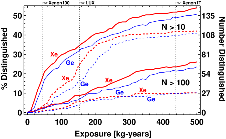
Figure 3: Distinguishability analysis in 500 kg-years. The number of degenerate pairs/percentage of the total that can be distinguished as a function of integrated exposure time. We plot exposure on germanium and xenon targets simultaneously. Heavy (red) lines are labeled for xenon, thinner (blue) lines are labeled for germanium. Solid lines have not been rescaled by the relic density ratio $r_{\chi}$, dashed lines have. The upper four lines are obtained by requiring only $N\geq 10$ recoil events for both models. The lower four lines are obtained by requiring $N\geq 100$ recoil events for both models. The predicted exposure after one year for three projected liquid xenon experiments is indicated by the vertical lines as labeled. Note that we assume 200 days of data-taking per calendar year with 80% of the mass from Table 2 used as a fiducial target mass.

Based on these two criteria, none of the 378 models would have been distinguished already in the Zeplin II, CDMS II or Xenon10 experiments – indeed none should have produced a detectable signal in any of these experiments. We do find nine models which would have given at least ten events in 316.4 kg-days of exposure time in the Xenon10 experiment, and five that would have given at least ten events in 397.8 kg-days of exposure time in the CDMS II experiment. These are models that could have been discovered at CDMS II (where no signal-like events were observed) or nearly discovered at Xenon10 (where ten signal-like events were reported). Yet all of these cases were ones in which the neutralino relic abundance was well below the value $\Omega_{\chi}{\rm h}^{2}=0.025$. After rescaling the value of $\rho_{\chi}$ from its nominal value of $\rho_{\chi}=0.3$ GeV/cm³ (or equivalently, the result of (9) for the differential rate) all of these models would have produced no events at either experiment. This is despite the fact that the naive expectation from Figure 2 is that at least a half-dozen models would have been detected at CDMS II, and at least one at Xenon10.

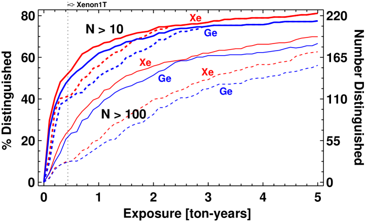
Figure 4: Distinguishability analysis in 5 ton-years. Same as Figure 3 for a much larger exposure time. The vertical line represents our projection for one year of data-taking in the future XENON1T experiment. Note that we assume 200 days of data-taking per calendar year with 80% of the mass from Table 2 used as a fiducial target mass.

In Figures 3 and 4 we plot the percentage of the 276 pairs that can be distinguished as exposure time is accumulated in xenon and germanium. Exposure time in Figure 3 is valued in units of kg $\times$ calendar-years and in units of tons $\times$ calendar-years in Figure 4. The separability criterion was $5\sigma$ and assumed an experimental error with no additional smearing ($f=0$) and no theoretical uncertainty. The upper four curves in the figures require $N\geq 10$ predicted recoil events for each model before being included in the total; the lower four curves require $N\geq 100$ predicted recoil events for each model. Solid lines are cases in which the local halo number density $n_{\chi}$ was not rescaled for models with $\Omega_{\chi}{\rm h}^{2}<0.025$. The dashed lines rescale the local density (and hence the differential interaction rate) by the parameter $r_{\chi}$. As a reference point we have included an estimate of the integrated exposure time after one calendar year of running for some of the projected liquid xenon experiments in Table 2. These estimates assume 200 days of data-taking per calendar year with 80% of the nominal masses in Table 2 being used as the fiducial mass.

	Mass Parameters (GeV)						LSP Wave Function
	$m_{N_{1}}$	$m_{N_{2}}$	$m_{C_{1}}$	$m_{\tilde{\tau}_{1}}$	$m_{h}$	$\mu$	$\widetilde{B}$%	$\widetilde{W}$%	$\widetilde{H}$%	$\Omega_{\chi}{\rm h}^{2}$
Point A	237	240	239	261	117.4	991	78%	21%	1%	0.0054
Point B	260	749	260	450	117.4	949	0%	99%	1%	0.0026

Table 3: Pair 212 of the 276 degenerate pairs. Some key parameters for the two models making up degenerate pair #212. This particular case is an example of a “squeezer” degeneracy, in the language of [6].

Generally speaking when two models are visible they are easily distinguished, at least under the idealized assumption of perfect theoretical control over the input nuclear matrix elements. Consider, for example, the pair of points described in Table 3. Both models are consistent with all experimental constraints, including those of (5). This model is typical of the set from Arkani-Hamed et al. In fact, it is of the sort that were dubbed “squeezers:” a case in which the mass difference between gauginos of the electroweak sector is small for one of two models, making the decay products from gaugino cascade decays too soft to be detected. The lepton-based signatures are accidently similar because of the compensating change in the stau masses. Both points predict a physically acceptable, if low, thermal relic abundance of neutralinos. The low values are due to the large wino-content of the LSP, and imply that detection rates should be scaled downward by factors of 0.22 for Point A and 0.1 for Point B. Consequently, despite relatively large spin-independent interaction cross sections of $\sigma_{\chi\,p}^{A}=3.61\times 10^{-45}$ cm² and $\sigma_{\chi\,p}^{B}=4.56\times 10^{-45}$ cm², neither would produce any interactions in current direct search experiments. We estimate that after one ton-year of exposure, a liquid xenon based experiment would collect $N_{A}=1310$ recoil events for Point A and $N_{B}=1517$ recoil events for Point B if we do not rescale their local relic density $n_{\chi}$. With rescaling these become $N_{A}=282$ and $N_{B}=157$. With these latter numbers, and assuming zero background contribution ($f=0$), these two signals differ by $6.4\sigma$. Even taking $f=0.5$ they still differ by $5.3\sigma$.

The above case is typical; in a world without theoretical uncertainties the limiting factor in distinguishing between these degenerate pairs is the requirement of 100 events total for each model in the pair. For example, with no rescaling of the local relic density and setting $f=0$ in (13) there are 231 pairs for which both models in the pair give 100 events in one ton-year of xenon exposure, versus 217 such pairs in germanium. If we require these signals to differ by two sigma the numbers become 190 and 176, respectively. Requiring five sigma significance only reduces these totals to 154 and 147. Now requiring five sigma significance and smearing the counts by a factor of $f=0.5$ only reduces the totals to 144 and 134. In fact, of these 154 pairs that can be distinguished in one ton-year of liquid xenon exposure (with $f=0$), the average separation significance is $21.8\sigma$! The equivalent number for the 147 pairs distinguishable in an equivalent exposure of germanium is $24.4\sigma$. As soon as both of the models surpass our threshold for a detectable “signal” they are almost always immediately distinguishable. As we will see below, this high degree of separability is an artifact of the assumption of perfect theoretical precision on the calculation of interaction cross-sections.

	With Density Rescaling
	Require 100 Events						Require 10 Events
		Xenon			Germanium			Xenon			Germanium
		$f=0$	$f=0.5$		$f=0$	$f=0.5$		$f=0$	$f=0.5$		$f=0$	$f=0.5$
	$3\sigma$	8	8		8	7	$3\sigma$	24	22		24	21
0.1 ton-yr	$5\sigma$	6	4		5	3	$5\sigma$	14	9		14	8
	$3\sigma$	79	71		69	58	$3\sigma$	164	148		157	136
1 ton-yr	$5\sigma$	52	43		48	37	$5\sigma$	112	81		105	73
	$3\sigma$	199	182		187	178	$3\sigma$	217	199		212	201
5 ton-yr	$5\sigma$	170	159		162	151	$5\sigma$	187	175		183	172

Table 4: Direct detection summary table. We give the number of pairs distinguishable after a given accumulated exposure in xenon or germanium, based on the integration ranges specified in the text. All numbers in this table were computed with interaction rates scaled by the quantity $r_{\chi}={\rm Min}(1,\,\Omega_{\chi}{\rm h}^{2}/0.025)$.

We summarize the numerical results of this section in Tables 4 and 5. We provide the number of model pairs that can be distinguished at either the $3\sigma$ or $5\sigma$ level in three different exposure times for xenon and germanium. We continue to assume that theoretical uncertainties are under control. In order to provide the reader with some context on the additional assumptions we have made, we provide the data using a threshold of 100 events and 10 events as well as calculating distinguishability with a conservative error ($f=0.5$) or assuming no background ($f=0$). Finally, we note that of the 77 model pairs we originally designated as “physical” in Section 2.2, 57 of them will be distinguished at the $5\sigma$ level (requiring a 100 event threshold) after one ton-year of exposure in xenon, assuming $f=0$ and without rescaling the local density of neutralinos. With rescaling only 3 of these “physical” models will be distinguished in one ton-year. Extending the exposure time to five ton-years increases these numbers to 65 out of 77 (no rescaling) and 31 out of 77 (with rescaling).

	Without Density Rescaling
	Require 100 Events						Require 10 Events
		Xenon			Germanium			Xenon			Germanium
		$f=0$	$f=0.5$		$f=0$	$f=0.5$		$f=0$	$f=0.5$		$f=0$	$f=0.5$
	$3\sigma$	51	41		49	41	$3\sigma$	116	102		111	98
0.1 ton-yr	$5\sigma$	36	29		32	25	$5\sigma$	81	69		77	63
	$3\sigma$	177	168		168	161	$3\sigma$	210	200		208	198
1 ton-yr	$5\sigma$	154	144		147	134	$5\sigma$	181	165		175	155
	$3\sigma$	242	235		240	234	$3\sigma$	242	235		240	234
5 ton-yr	$5\sigma$	224	216		217	211	$5\sigma$	224	216		217	211

Table 5: Direct detection summary table. Same as Table 4, only without scaling interaction rates.

Tables 4 and 5 illustrate the incredible power of the next-generation of dark matter direct detection experiments. The improvements to (already good) background rejection mechanisms will make these experiments very accurate counters – but without equivalent improvements on the issue of theoretical inputs the utility of these measurements will be severely degraded. This point was raised by Ellis et al. [33], who studied the variation in the prediction for $\sigma^{\mathrm{SI}}_{\chi p}$ arising from differing input values of the $\pi\,N$ $\Sigma$-term. We computed the value of $\sigma^{\mathrm{SI}}_{\chi p}$ for the 378 models of this study using the range of input parameters considered in Ref. [33], arriving at a typical variation of approximately 50% for the interaction cross-section. This is similar to the observed variation of Ellis et al., as well as others who have undertaken similar investigations [34]. Let us consider an additional theoretical error proportional to the calculated cross-section

$$\left(\delta\sigma^{\mathrm{SI}}_{\chi}\right)_{\rm theor}=\epsilon\times\sigma^{\mathrm{SI}}_{\chi}$$ (14)

which is to be added in quadrature to the statistical errors considered previously. In Table 6 we show the degradation in the number of distinguishable pairs that arises from considering $\epsilon\neq 0$. The entries in Table 6 should be compared to those of the right panel in Figure 4; we require at least 10 signal events in one (or five) ton-years of xenon exposure. The interaction rates in this table were rescaled for cases of low predicted thermal relic density. Clearly if theoretical uncertainties stay at their present level (with roughly 50% uncertainty in the cross-section predictions) then it will be impossible to distinguish models with direct detection experiments – even after five ton-years of exposure and requiring only $3\sigma$ separation. If the uncertainty in the $\pi\,N$ $\Sigma$-term can be reduced so as to generate only a 10% theoretical uncertainty in $\sigma^{\mathrm{SI}}_{\chi p}$ the ability to distinguish models will still be significantly reduced, but some hope for separating models will remain. For this reason we strongly echo the call made by Ellis et al. for further experimental work aimed towards reducing these uncertainties.

	Require 10 Events, Xenon
		$\epsilon=0$	$\epsilon=0.1$	$\epsilon=0.25$	$\epsilon=0.5$
	$3\sigma$	164	118	13	0
1 ton-yr	$5\sigma$	112	46	0	0
	$3\sigma$	217	149	25	0
5 ton-yr	$5\sigma$	187	77	0	0

Table 6: Effect of theoretical uncertainties associated with nuclear matrix elements. We give the number of pairs distinguishable after a given accumulated exposure in xenon when an additional theoretical uncertainty of the form of (14) is included. We take the experimental error to be purely statistical ($f=0$) and require 10 signal events. All numbers in this table were computed with interaction rates scaled by the quantity $r_{\chi}={\rm Min}(1,\,\Omega_{\chi}{\rm h}^{2}/0.025)$.

4 Gamma Ray Experiments

Direct detection experiments measure the presence of relic neutralinos at the location of the earth. Indirect detection of relic neutralinos involves looking for the products of neutralino pair annihilation processes far from the earth’s location. Given a supersymmetric model, the rate for annihilation into various final states can be computed as a function of parameters such as the neutralino mass $m_{\chi}$. Of these possible final states, photons in the gamma ray energy regime are unique in that they are uninfluenced by galactic magnetic fields and travel largely unimpeded from their source. This allows gamma ray observatories to concentrate on areas of the sky likely to have a high relic neutralino density – such as the center of our galaxy. This is important since the rate for annihilation processes scales like the square of the local density $\rho_{\chi}$. Photons can be produced as part of decay chains (for example, from the decays of neutral pions in hadronic decays) or directly through loop-induced diagrams. The former contribute to a continuous general spectrum of photons and are thus more difficult to distinguish from astrophysical backgrounds. But direct production of two photons – or production of a single photon in association with a Z-boson – through loop-diagrams offers the possibility of a monochromatic spectrum that can more easily be distinguished from the background [35]. The trade-off is a reduction in rate relative to the continuous photon rate.

The rate of gamma ray photons observed at the earth’s location is sensitive to the radial dependence of the relic neutralino density profile assumed. The majority of the profiles considered in the literature can be described by a common parameterization

$$\rho_{\chi}(r)=(\rho_{\chi})_{0}\frac{\left(r/r_{0}\right)^{-\gamma}}{\left[1+\left(r/a\right)^{\alpha}\right]^{\frac{\beta-\gamma}{\alpha}}}\left[1+\left(\frac{r_{0}}{a}\right)^{\alpha}\right]^{\frac{\beta-\gamma}{\alpha}}\,,$$ (15)

where $r_{0}$ is roughly the distance between the earth and the galactic center and the normalization constant $(\rho_{\chi})_{0}$ is typically taken to be 0.3 GeV/cm³. It is this parameter which is rescaled for those models with $\Omega_{\chi}{\rm h}^{2}<0.025$. The function in (15) is integrated along the line of sight between the earth and the observed object – for us this will be the galactic center. All of the physics of the halo model chosen is therefore sequestered to a single overall scaling parameter $J(\psi)$

$$J(\psi)=\frac{1}{8.5\,{\rm kpc}}\left(\frac{1}{0.3~{}\mathrm{GeV}\,{\rm cm}^{3}}\right)^{2}\int_{\rm line\,of\,sight}ds(\psi)\,\rho^{2}_{\chi}(r)\,$$ (16)

with $s(\psi)$ being a parameter running along the ray to the observed object, making an angle $\psi$ relative to the galactic center. For observations of the galactic center $\psi=0$. If the quantity $\Delta\Omega$ represents the finite angular resolution of a given detector, then the quantity (16) is integrated over a spherical region of solid angle $\Delta\Omega$ centered on $\psi=0$. The average value of $J(\psi)$ over this region

$$\left\langle J(\psi)\right\rangle_{\Delta\Omega}=\frac{1}{\Delta\Omega}\int_{\Delta\Omega}d\Omega^{\prime}\,J(\psi^{\prime})$$ (17)

is often denoted $\overline{J}(\Delta\Omega)$ and is handy for comparing rates computed with different halo model assumptions.

Different choices for the parameter set $(a,\,r_{0},\,\alpha,\,\beta,\,\gamma)$ common in the literature can change the resulting value of $\overline{J}(\Delta\Omega)$ (and hence the predicted gamma ray flux) by several orders of magnitude. This is by far the greatest source of uncertainty in making definitive statements about the ability of gamma ray experiments to distinguish between competing theories. Indeed, values of $\overline{J}(\Delta\Omega)\mathrel{\hbox to0.0pt{\raise 2.15277pt\hbox{$>$}\hss}{\lower 2.15277pt\hbox{$\sim$}}}{\rm few}\times 10^{4}$ will be required if any of the current or proposed experiments are to observe a signal at all. In this paper we will therefore primarily consider the model of Navarro, Frank and White (NFW) [36] as well as a modified NFW profile that takes into account the effect of baryons (a so-called “adiabatic compression” (AC) model) [37, 38]. On occasion we will also refer to a more singular profile by Moore et al. [39], also with the effects of adiabatic compression, which is more favorable for the prospects of indirect dark matter detection at gamma ray experiments. The parameters associated with these three models, as well as the computed values of $\overline{J}(\Delta\Omega)$ for the galactic center are given in Table 7. These values can be used to scale our subsequent results for comparison to other profile models.

Model	$r_{0}$ (kpc)	$a$ (kpc)	$\alpha$	$\beta$	$\gamma$	$\overline{J}(10^{-5}\,{\rm sr})$
NFW	8.0	20.0	1	3	1	$1.2644\times 10^{4}$
NFW + AC	8.0	20.0	0.8	2.7	1.45	$1.0237\times 10^{6}$
Moore + AC	8.0	28.0	0.8	2.7	1.65	$3.0896\times 10^{8}$

Table 7: Halo model parameters. The parameters which define the three halo models we will consider in this work and the resulting value of the parameter $\overline{J}(\Delta\Omega)$ for $\Delta\Omega=10^{-5}$ sr. We will primarily consider the NFW halo profile with adiabatic compression in what follows.

Before proceeding we emphasize that we will treat the three input values for $\overline{J}(\Delta\Omega)$ in Table 7 as discrete possibilities for this crucial input parameter. It is unclear whether this is a reasonable assumption, though it is commonly made in the literature. As we will argue at the end of this section, consistency between any post-LHC supersymmetric model and any future signal of dark matter annihilation at the galactic center will likely single out only one of these profile models given their wide disparity in $\overline{J}(\Delta\Omega)$ values. But if these values merely represent signposts along a continuum of possible $\overline{J}(\Delta\Omega)$ it is unclear how indirect detection of dark matter via annihilation into photons will ever be able to distinguish between two candidate supersymmetric models – at least in the absence of other, orthogonal data from other cosmological observations. The situation would then be analogous to trying to separate two theories on the basis of the number of trilepton events at the LHC, but with a luminosity that is uncertain by as much as four orders of magnitude! Clearly, then, maximizing the value of future experimental observations will require much better knowledge of the uncertainties associated with numbers such as those in Table 7. We will continue this section under the original assumption that only one of these models is correct and that the prediction for $\overline{J}(\Delta\Omega)$ associated with that model is exact, returning to the issue of theoretical uncertainty at the end of the section.

The differential flux of photons from neutralino annihilation at the earth’s location is then given by

$$\frac{d\Phi_{\gamma}(E_{\gamma})}{dE_{\gamma}}=\sum_{i}\frac{\left\langle\sigma_{i}v\right\rangle}{4\pi m_{\chi}^{2}}\frac{dN^{i}_{\gamma}}{dE_{\gamma}}\int_{\rm line\,of\,sight}ds(\psi)\,\rho^{2}_{\chi}(r)\,,$$ (18)

where the summation is over all possible final states, $\sigma_{i}$ is the annihilation cross-section into that final state, and $dN^{i}_{\gamma}/dE_{\gamma}$ is the differential spectrum of photons produced in the decay channel labeled by the index $i$. Replacing the halo integral in (18) by (17) gives

$$\frac{d\Phi_{\gamma}(E_{\gamma})}{dE_{\gamma}}=0.94\times 10^{-13}\sum_{i}\frac{dN^{i}_{\gamma}}{dE_{\gamma}}\left(\frac{\left\langle\sigma_{i}v\right\rangle}{10^{-29}\,{\rm cm}^{3}\,{\rm s}^{-1}}\right)\left(\frac{100~{}\mathrm{GeV}}{m_{\chi}}\right)^{2}\overline{J}(\Delta\Omega)\Delta\Omega$$ (19)

in units of photons/cm²/s/GeV. The final step is to perform an integration over the energy range relevant to the particular experiment. The continuous gamma ray spectrum from neutralino annihilation has a sharp cut off at the mass of the neutralino $m_{\chi}$. We therefore integrate (19) from some sensitivity threshold $E_{\rm min}$ to $E_{\rm max}$, where $E_{\rm max}$ is the smaller of the mass of the neutralino or the upper limit of the experiment’s energy sensitivity. Note that for monochromatic lines produced by processes $\chi_{0}\,\chi_{0}\to\gamma\,\gamma$ and $\chi_{0}\,\chi_{0}\to\gamma\,Z$ no such integration is necessary and $dN^{i}_{\gamma}/dE_{\gamma}$ in (19) is replaced by $N_{\gamma}=2$ and $N_{\gamma}=1$ for these two cases, respectively.

In this section we will consider two broad classes of gamma ray observatories which are operational now or will become so in the near future: space-based satellites such as the GLAST LAT [40] and ground based atmospheric Cherenkov telescopes (ACTs) such as CANGAROO [41], HESS [42], MAGIC [43] and VERITAS [44]. The two classes have different strengths and weaknesses, making them suited for different signals of dark matter annihilation. Space-based experiments can observe nearly continuously, while ground based experiments can collect data only on dark, cloudless nights. On the other hand these ACTs cover a much larger effective area $A_{\rm eff}$ of the sky than the GLAST LAT. The GLAST experiment will be sensitive to photon energies from $\mathcal{O}(10\,{\rm MeV})$ to about 300 GeV – a photon energy range much lower than that of the ACTs whose threshold energies are in the range 50-100 GeV, if not higher. The lower energy region is more suited for measurements of the continuous gamma ray flux arising from neutralino annihilations. The masses of the neutralino LSP in our 378 models fall in the range

$$98~{}\mathrm{GeV}\leq m_{\chi}\leq 557~{}\mathrm{GeV}$$ (20)

with over 85% having a mass less than 300 GeV. We will therefore discuss the continuous gamma ray spectrum only in the context of the GLAST experiment. However, the two monochromatic fluxes associated with di-photon and photon/Z-boson final states have associated photon energies

$$E_{\gamma\gamma} = m_{\chi}$$

$$E_{\gamma Z} = m_{\chi}-M_{Z}^{2}/4m_{\chi}\,,$$ (21)

respectively. For these signals we will only consider ACT experiments; GLAST is sensitive to many of the relevant energy values but the flux is too small to give an appreciable rate in all but the Moore (AC) halo profile. In Table 8 we list the relevant experimental parameters for GLAST and a generic ACT based roughly on the characteristics of the HESS and VERITAS experiments. We will use these two experimental configurations in our analysis.

	$E_{\rm min}$	$E_{\rm max}$	$\sigma_{E}/E$	$A_{\rm eff}$	$\Delta\Omega$
GLAST	50 MeV	300 GeV	10%	$1\times 10^{4}$ cm2	$1\times 10^{-5}\,{\rm sr}$
ACT	100 GeV	10 TeV	15%	$3\times 10^{8}$ cm2	$1\times 10^{-5}\,{\rm sr}$

Table 8: Gamma Ray Experiments. For the analysis presented in this section we consider two gamma ray observatories: the GLAST satellite-based experiment and a generic atmospheric Cherenkov telescope.

An important distinction between the gamma ray experiments and the nuclear recoil experiments of Section 3 is in the nature of backgrounds. We argued in the previous section that direct detection experiments expect to achieve a high degree of background rejection in future incarnations. For our analysis of distinguishability we assumed a small (but non-vanishing) rate for misidentifying nuclear recoils. The rates we have in mind for these experiments were in the range of 1 - 10 events per experiment per year. This motivated the requirement of at least 10 to 100 nuclear recoil events observed for a given model before a definitive statement is made. There is no similarly successful method for discriminating between photons resulting from neutralino annihilation and those that arise from other astrophysical processes that generate gamma rays of the same energy range. As a result, indirect detection of relic neutralinos implies observing an excess of high energy photons above some background rate that can be quite substantial. Accurate and believable modeling of this background photon rate is therefore crucial for making measurements that can be used to distinguish between two models in a degenerate pair.

Photons in the gamma ray energy regime are produced from a number of sources. These include high energy cosmic ray proton collisions with helium gas which produces $\pi^{0}$’s, interactions of electrons with galactic radiation via inverse Compton scattering and bremsstrahlung processes from accelerated charges [45]. For energies in the broad range $100\,{\rm MeV}\mathrel{\hbox to0.0pt{\raise 2.15277pt\hbox{$<$}\hss}{\lower 2.15277pt\hbox{$\sim$}}}E_{\gamma}\mathrel{\hbox to0.0pt{\raise 2.15277pt\hbox{$<$}\hss}{\lower 2.15277pt\hbox{$\sim$}}}1\,{\rm TeV}$ relevant for neutralino annihilation, the sum of these processes produces a differential spectrum typically modeled by a power law of the form [46]

$$\frac{d^{2}\Phi^{\rm bkg}_{\gamma}}{d\Omega dE_{\gamma}}=\left(\frac{d\Phi^{\rm bkg}_{\gamma}}{d\Omega dE_{\gamma}}\right)_{0}\,\left(\frac{E_{\gamma}}{1~{}~{}\mathrm{GeV}}\right)^{-2.7}\,$$ (22)

where $(d\Phi^{\rm bkg}_{\gamma}/d\Omega\,dE_{\gamma})_{0}$ has units of photons/cm²/s/sr/GeV and serves as a normalization for the spectrum. A reasonable value for this parameter would be approximately

$$\left(\frac{d^{2}\Phi^{\rm bkg}_{\gamma}}{d\Omega dE_{\gamma}}\right)_{0}\simeq 9\times 10^{-5}\,{\rm photons/cm^{2}/s/sr/GeV}$$ (23)

in the direction of the galactic center. Integrating (22) with normalization (23) over a typical range relevant to GLAST of $1~{}\mathrm{GeV}\leq E_{\gamma}\leq 200~{}\mathrm{GeV}$, and using $\Delta\Omega=10^{-5}$, one obtains approximately 100 background photons per m²-year of exposure. This suggests that any model capable of producing a flux from neutralino annihilations of the order of $\Phi_{\gamma}\simeq 10^{-10}\,{\rm photons/cm^{2}/s}$ at GLAST (when integrated from a threshold energy of 1 GeV) should be detectable above background. Such estimates are often quoted in the literature [47, 48].

However, there are reasons to be concerned about how well this background rate is understood [45, 49]. Observations from the satellite-based EGRET experiment [50] indicated a higher-than-expected photon flux in the energy range of 100 MeV to approximately 10 GeV in the direction of the galactic center. Furthermore, earth-based ACT experiments HESS [51], VERITAS [52], CANGAROO [53] and MAGIC [54] also observed an anomalously large gamma-ray source in the direction of the center of the galaxy for higher energy photons ($200~{}\mathrm{GeV}\mathrel{\hbox to0.0pt{\raise 2.15277pt\hbox{$<$}\hss}{\lower 2.15277pt\hbox{$\sim$}}}E_{\gamma}\mathrel{\hbox to0.0pt{\raise 2.15277pt\hbox{$<$}\hss}{\lower 2.15277pt\hbox{$\sim$}}}10~{}\mathrm{TeV}$). It is likely that both the EGRET data and the ACT data represent newly identified point-like sources near the galactic center [55, 56]. Given the fine angular resolution available with GLAST it should be possible to subtract these point sources from the more diffuse signal expected from neutralino annihilation. This issue was the subject of a recent study by Dodelson, Hooper and Serpico [57] in which the separation of dark matter signals from background sources was performed using both spectral information as well as angular information. We will loosely follow the example of [57] for our treatment of backgrounds in light of the EGRET/ACT data.

We therefore consider two different background estimations. The first is simply the one represented by the power law in (22) with normalization (23). This is the standard case studied in the literature and we will refer to this case as the “low” background. For the second background estimation we will use (22) and (23) as a baseline but then take into account the EGRET data by adding to it an additional contribution modeled by [57]

$$\frac{d\Phi^{\rm EG}_{\gamma}}{dE_{\gamma}}=2.2\times 10^{-7}\,\times{\rm exp}\left(-\frac{E_{\gamma}}{30~{}\mathrm{GeV}}\right)\times\left(\frac{E_{\gamma}}{1~{}\mathrm{GeV}}\right)^{-2.2}\,\,{\rm photons/cm^{2}/s/GeV}\,.$$ (24)

For the high energy ACT sources we add an additional contribution modeled by [57]

$$\frac{d\Phi^{\rm ACT}_{\gamma}}{dE_{\gamma}}=1.0\times 10^{-8}\,\times\left(\frac{E_{\gamma}}{1~{}\mathrm{GeV}}\right)^{-2.25}\,\,{\rm photons/cm^{2}/s/GeV}\,,$$ (25)

for energies $E_{\gamma}\geq 200~{}\mathrm{GeV}$. In practice we will only integrate the GLAST signal up to 200 GeV, so this second contribution in (25) will be relevant only as background to monochromatic signals in the generic ACT experiment of Table 8. This set of assumptions we will refer to as the “high” background. We note again that these additional contributions (24) and (25) presumably represent point sources which may be reliably removed from the data given the angular resolution of GLAST. For our simple study we will not bin the data in solid angle, and perform only a crude binning in energy. We therefore consider treating (24) and (25) as additional diffuse contributions to be a reasonable and conservative assumption.

Let us begin with the continuous differential spectrum and the GLAST experiment. Following [57] we will attempt to take into account the shape of this spectrum as part of our analysis. For each model we use DarkSUSY to compute the differential photon flux from (19) in 1 GeV increments over the energy range $1~{}\mathrm{GeV}\leq E_{\gamma}\leq 200~{}\mathrm{GeV}$. From this information we create an interpolating function which is then integrated over six energy bins: 1 - 10 GeV, 10 - 30 GeV, 30 - 60 GeV, 60 - 100 GeV, 100 - 150 GeV, and 150 - 200 GeV. For each model we also compute a total integrated flux by integrating over the entire range $1~{}\mathrm{GeV}\leq E_{\gamma}\leq 200~{}\mathrm{GeV}$. To say that two different signals are detectable and distinguishable after a certain observation time we require the following simultaneous conditions:

1. The total number of gamma ray photons $N_{\gamma}$ collected by the experiment over the full energy range $1~{}\mathrm{GeV}\leq E_{\gamma}\leq 200~{}\mathrm{GeV}$ must satisfy $N_{\gamma}>100$. We require this to be true of both models in the model pair.

2. We require in addition that a significant excess of gamma ray photons above background is observed in multiple, adjacent energy bins. The premise behind this requirement is the desire to have some spectral information on the component of the flux arising from dark matter annihilation to better separate this source from other astrophysical sources. Specifically, if $i=1,\dots,6$ labels our six energy bins, then we demand $N_{i}>m\sqrt{N_{i}^{\rm bkg}}$ for at least three adjacent bins. Here $N_{i}$ is the number of photons observed in that energy bin, $N_{i}^{\rm bkg}$ is the expected background count (computed either with the “low” or the “high” background model), and $m$ is the significance level in units of signal/$\sqrt{{\rm bkgrnd}}$. In what follows we will demand $m=2$.

3. If the above two conditions are satisfied by models $A$ and $B$ then we will say that the two potential signals are detectable. We will further say that they are distinguishable if the condition $|N_{i}^{A}-N_{i}^{B}|>n\sqrt{N_{i}^{A}+N_{i}^{B}+2N_{i}^{\rm bkg}}$ holds for at least three adjacent bins, simultaneously. Results will be given for significance levels $n=3$ and $n=5$.

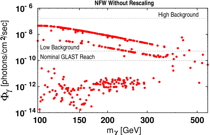
Figure 5: Integrated photon flux for NFW profile and no density rescaling. The differential photon flux is integrated over the energy range $1~{}\mathrm{GeV}\leq E_{\gamma}\leq 200~{}\mathrm{GeV}$ for the NFW profile. In this plot none of the rates have been rescaled in accordance with the predicted thermal relic density. The flux from background sources are indicated by the horizontal dotted lines for our “low” and “high” background models. We also give the nominal sensitivity threshold claimed by the GLAST collaboration.

The majority of studies in the literature focus on only the first of the above items. Since the total (integrated) flux $\Phi_{\gamma}(E_{\gamma}\geq 1~{}\mathrm{GeV})$ is such a commonly considered variable we begin here. In Figure 5 we plot the integrated flux from $1~{}\mathrm{GeV}\leq E_{\gamma}\leq 200~{}\mathrm{GeV}$ arising from dark matter annihilations as a function of the neutralino mass $m_{\chi}$ in the NFW halo profile. The typical integrated flux values for our 378 models are on the order of $10^{-11}$ photons/cm²/sec if we rescale the local halo density by the factor $r_{\chi}$, as is the default setting in DarkSUSY. Therefore if any significant flux is to be produced at all with the NFW profile then we must assume that the halo density $\rho_{\chi}(r)$ is not rescaled. That was the assumption that went into producing Figure 5. Our two background estimations have been integrated over the same energy range and are shown as the horizontal dotted lines. Note that the “low” background rate corresponds well with the typically quoted GLAST sensitivity limit of $\Phi_{\gamma}=10^{-10}$ photons/cm²/sec [47]. An alternative – and perhaps more reasonable – set of assumptions is to add the prospect of adiabatic compression but include the effects of halo density rescaling. With these assumptions we get the distribution in Figure 6. Clearly more favorable assumptions could be made; for example the profile of Moore et al. with adiabatic compression would boost these numbers by a factor of roughly 30.

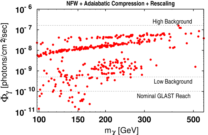
Figure 6: Integrated photon flux for NFW profile + adiabatic compression. Same as Figure 5 but with the addition of adiabatic compression. In this plot we have rescaled the annihilation rate by the factor $r_{\chi}$.

After converting the differential fluxes into actual photon counts as described above, we ask how well the model pairs can be separated as GLAST observation time is integrated. Our results are shown in Figure 7 as a function of integrated time-on-target in units of m²-years. Note that as in the case of direct detection experiments one calendar year of the GLAST mission does not necessarily produce 1 m²-year of integrated observation since, for example, the telescope will not be directed at the galactic center continuously. The figure is computed for the NFW halo profile with adiabatic compression. The lower two curves rescale the local halo density for those models where $\Omega_{\chi}{\rm h}^{2}<0.025$ while the upper two curves have no such rescaling. Dashed curves count the number of separable models using the low background, while solid curves use the higher EGRET-normalized background. With the most conservative assumptions – rescaling the halo density for low $\Omega_{\chi}{\rm h}^{2}$ models and using the higher background estimate – only 20% of the model pairs are distinguished even after 5 m²-years. Assuming only the “low” background of (22) and (23) gives a figure above 40%. We feel this is a reasonable, if conservative, estimate of the power of the GLAST experiment to distinguish between degenerate pairs in the event that signals are visible at all above background.

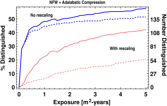
Figure 7: Distinguishability analysis at GLAST. The lower two curves rescale the local halo density by the factor $r_{\chi}$ while the upper two curves have no rescaling. The solid lines give the number of distinguished pairs using the “low” background estimate, while dashed lines are for the “high” background estimate.

We summarize the results of the continuous gamma ray observables in Table 9. Four different halo assumptions are listed: NFW with rescaling the halo density, NFW + adiabatic compression (with and without rescaling the halo density), and Moore et al. with halo density rescaling. All results assume $m=2\sigma$, but we consider both a high and low background assumption with either $3\sigma$ or $5\sigma$ separation criterion.

				NFW		NFW		Moore
		NFW		adiab. comp.		adiab. comp.		adiab. comp.
		not rescaled		rescaled		not rescaled		rescaled
Background:		low	high	low	high	low	high	low	high
	$3\sigma$	4	0	98	29	148	133	220	165
1 m2 yr	$5\sigma$	0	0	60	14	131	122	196	151
	$3\sigma$	22	0	135	49	160	145	232	186
3 m2 yr	$5\sigma$	9	0	95	33	144	134	185	173
	$3\sigma$	35	0	147	62	167	147	207	194
5 m2 yr	$5\sigma$	13	0	111	42	154	139	194	183

Table 9: Integrated gamma ray flux summary table. The number of pairs distinguishable at the $n=3\sigma$ and $5\sigma$ level are listed for three different integrated exposures at GLAST. The four halo models assumptions are NFW without halo rescaling, NFW plus adiabatic compression (with and without halo rescaling) and Moore et al. with halo rescaling. We consider both the low (or standard) background estimate as well as an EGRET-normalized higher background estimate. Theoretical uncertainties associated with these halo models are neglected in this table.

For the case of the monoenergetic signals coming from loop-induced dark matter annihilations the background at these higher photon energies ($E_{\gamma}\mathrel{\hbox to0.0pt{\raise 2.15277pt\hbox{$>$}\hss}{\lower 2.15277pt\hbox{$\sim$}}}100~{}\mathrm{GeV}$) is substantially reduced over the continuous differential signal considered just above. For this case we include the “low” background of (22) and (23) plus the additional higher energy source of (25). Together these provide a very small rate, particularly when integrated over the narrow window $E_{\gamma\gamma}\pm\sigma_{E}^{\rm ACT}$ or $E_{\gamma Z}\pm\sigma_{E}^{\rm ACT}$ relevant for these monochromatic signals. For example, if we integrate the background rate for a $1\sigma$ region about $E=200~{}\mathrm{GeV}$ we get $\mathcal{O}(10^{-2})$ events per m²-year for the low background and $\mathcal{O}(1)$ events per m²-year for the higher background which includes (25). Despite this pleasant fact, the signal rates are very small as well. Typical annihilation rates through these loop-induced processes are roughly $10^{-3}$ to $10^{-4}$ times those for the tree-level processes. For the NFW profile with density rescaling typical event rates in our model set are $\sim 0.02$ photons/m²-year. Without rescaling this increases to $\sim 10$ photons/m²-year. Typical rates for other halo profiles can be found multiplying these numbers by the ratios of $\overline{J}(10^{-5}\,{\rm sr})$ values found in Table 7.

Given the relatively low background rate we will require at least $N_{\gamma}=10$ photons collected within $\pm\sigma_{E}^{\rm ACT}$ of the expected signal(s) at $E_{\gamma\gamma}$ and $E_{\gamma Z}$. To say two signals can be separated we continue to require that both can first be conclusively detected. We therefore demand that $N_{i}>m\sqrt{N_{i}^{\rm bkg}}$ where $i=\gamma\gamma$ or $\gamma\,Z$, the background is the “low” background plus the ACT-contribution of (25), and we will require a significance of $m=5$. However, the limiting factor in our ability to distinguish models in any given pair will not be signal significance but energy resolution.

For a particular model with a given $m_{\chi}$ value the energies of the two possible annihilation lines are given by (21). For an energy resolution of 15% these two lines can be resolved only for cases in which $m_{\chi}\mathrel{\hbox to0.0pt{\raise 2.15277pt\hbox{$<$}\hss}{\lower 2.15277pt\hbox{$\sim$}}}105~{}\mathrm{GeV}$. As this criteria is met by only a handful of the models in our set we will therefore consider a single line whose peak is at the average of the two energies in (21): $\overline{E}=(E_{\gamma\gamma}+E_{\gamma Z})/2$. We will then define two models to be distinguished if the two values $\overline{E}^{A}$ and $\overline{E}^{B}$ are separated by $n\,\sigma_{E}$, where $\sigma_{E}/E=0.15$, for a particular requirement on the significance $n$. For these degenerate model pairs the LSP masses $m_{\chi}$ for the two models are often very similar – implying that two values of $\overline{E}$ are typically separated by no more than one standard deviation for an energy resolution of 15%. This makes separating models extremely challenging in this arena. For example, let us take the case of the NFW halo profile with adiabatic compression, rescaling the local halo density by the ratio $r_{\chi}$. If we consider an integrated exposure of 500 m²-years at our generic ACT (equivalent to about 200 hours of data taking at 75% of the $A_{\rm eff}$ value in Table 8) then in 161 of the 276 pairs both of the models would produce detectable monochromatic signals above the “high” background of (25). Yet in only 67 pairs were the two central values $\overline{E}$ resolvable at the $1\sigma$ level. Requiring $2\sigma$ resolution reduced this number to only 23 pairs. If an energy resolution comparable to the GLAST experiment of 10% could be achieved, these numbers would roughly double. A summary of what is possible for varying levels of integrated exposure at a generic ACT is given in Table 10. As the table suggests, the efficacy of ACTs in distinguishing between models using monochromatic signals quickly saturates – those model pairs with sufficiently large $m_{\chi}$ mass differences as to be separated at a given significance level achieve $S/\sqrt{B}\geq 5$ within 100-200 m²-years of exposure.

ACT Exposure	Rescaled			Not Rescaled
	$1\sigma$	$2\sigma$	$3\sigma$	$1\sigma$	$2\sigma$	$3\sigma$
100 m2-years	51	14	3	66	23	10
500 m2-years	67	23	10	95	25	11
1000 m2-years	68	23	10	109	33	12

Table 10: Distinguishing pairs using monochromatic signals. The number of pairs that can be differentiated for varying amounts of integrated exposure are given for the generic ACT of Table 8. An NFW halo profile with adiabatic compression has been assumed. In all cases we use the background estimation of (25) with ${\rm signal}/\sqrt{\rm bkgrnd}\geq 5$. The two lines $\overline{E}^{A}$ and $\overline{E}^{B}$ are required to be separated by $n\,\sigma_{E}$, where $\sigma_{E}/E=0.15$ and we consider $n=1$, 2 and 3.

Returning to the issue of uncertainties in the halo model, it is reasonable to ask whether the appearance of an indirect signal for dark matter (whether it be a monochromatic line signal or the overall integrated gamma ray flux from the galactic center) can tell us anything about the supersymmetric model given the wide range of $\overline{J}(\Delta\Omega)$ values listed in Table 7. As mentioned earlier we believe the answer would be “no” in the absence of other data. But the assumption in this paper has been that we have two candidate models that have been constructed from the LHC data. For a given halo profile these models make two concrete predictions for the signals considered in this section. We have been asking whether the experiments considered here have the inherent power to resolve these predictions. The result of this section is that, given enough statistics, the answer is typically yes. It is important to note that the normalizations parameterized by $\overline{J}(\Delta\Omega)$ differ from one another by two orders of magnitude. Only two pairs of models in our study gave predictions that differed by this much or more for the integrated gamma ray flux – and no pairs differed by this amount for the monochromatic predictions. In fact, 252 of the 276 pairs of models gave predictions for the integrated gamma ray fluxes that differed by less than an order of magnitude. If we assume that the choices in Table 7 should be treated as a discrete set of possibilities then the size of any observed signal at GLAST or some future ACT experiment will likely pick out only one halo profile as reasonable if a fit is to be made to our post-LHC degenerate models.

Alternatively, if we treat the quantity $\overline{J}(\Delta\Omega)$ as an undetermined free parameter we can ask how well we would need to know the value of this parameter a priori to be able to distinguish the pairs of models in our list. To investigate this question we computed the total integrated gamma ray flux from the galactic center between the energy ranges of 1 GeV to 200 GeV, using the $\overline{J}(\Delta\Omega)$ value for GLAST for the NFW profile with adiabatic compression. We then converted this flux into a numerical count for our model pairs assuming no halo rescaling and 3 m²-years of exposure. We then asked how many model pairs could be separated at the $3\sigma$ level assuming the value of $\overline{J}$ was uncertain by an amount

$$\left(\delta\overline{J}\right)_{\rm theor}=\epsilon\times\overline{J}(\Delta\Omega)\,,$$ (26)

analogous to the consideration of nuclear matrix element uncertainties in Section 3. If we allow a 5% error in the input value of $\overline{J}(\Delta\Omega)$ then we can separate 152, 102 and 22 model pairs out of 276 for the cases of no background, low background, and high background, respectively. These numbers should be compared with the entries in the corresponding column of Table 9. The number of separable model pairs drops steadily, reaching zero for $\epsilon\simeq 0.32$ (low background) and $\epsilon\simeq 0.26$ (high background). Clearly, then, the theoretical modeling that goes into producing the values in Table 7 will need to be accurate to the 5-10% range to truly be able to separate post-LHC candidate supersymmetric models from gamma-ray observations alone.

5 Conclusions

If supersymmetry is relevant to the physics of the electroweak scale then it is very likely to be discovered in the near future at the LHC. Yet if the results of [6] are indicative of general supersymmetric theories then it is also likely that more than one supersymmetric model (or low energy parameter set) will be a reasonable fit to the ensemble of LHC measurements that will be made. In such a scenario the challenge to the high energy community will be to find orthogonal information that will be effective in breaking these degeneracies. If the lightest supersymmetric particle is stable then it is reasonable to imagine that it will be detected at future dark matter experiments. It is therefore instructive to consider how well measurements in this area serve to provide the needed orthogonal data.

In the current work we have considered only a subset of the experimental data that might be available over the next decade in the area of direct and indirect detection of dark matter neutralinos. However taken together these signals are sufficient to separate a large number of the degenerate pairs of Arkani-Hamed et al., even when rather conservative assumptions are made. Unfortunately this statement comes with a large caveat: the ability to distinguish between models will depend on certain theoretical inputs being better understood. For example, if superpartners exist at the electroweak scale and the LSP is stable then it is almost certain that a one-ton liquid xenon detector will eventually see a neutralino-recoil signal. But determining whether that signal was consistent with only one of two competing SUSY models (our original thought experiment) will be impossible without much better knowledge of the nuclear matrix elements that appear in the cross-section calculation. In this work we have made the assumption that such knowledge can indeed be obtained within the ten year time horizon we imagine between now and any future ILC experiment.

Another theoretical uncertainty is the imperfect knowledge of the dark matter halo in our galaxy – both the local density near the earth as well as the dependence of the halo density as a function of position from the galactic center. These quantities are fundamental inputs to any theoretical prediction, and as we have seen they can vary over larger ranges than other (in principle tractable) theoretical uncertainties. The existence of this ambiguity is an inherent property of cosmological observations; experiments will measure count rates which require both a particle physics model ($\left\langle\sigma v\right\rangle$) and an astrophysics model ($\overline{J}(\Delta\Omega)$) as inputs. Our theoretical control over the former – particularly in a post-LHC world – will likely be much better than over the latter. But this need not imply that dark matter signals have nothing to tell us about supersymmetric models. It is likely true that on their own such signals will be unable to establish any particular SUSY model as the correct one. But if any future dark matter signal proves to be consistent with what will be known at the LHC, for reasonable input assumptions, then this will be powerful (if indirect) evidence in favor of those assumptions. If, in addition, the observed signal is consistent with only one of a pair of predictions based on those same assumptions then we can reasonably claim that the dark matter signal in question has resolved a potential degeneracy. Of course if any future signal cannot be made consistent with a post-LHC candidate model, or is consistent only with unrealistic input assumptions, then no such resolving power exists.

With this philosophy in mind, we summarize the effect of all experiments considered in this work in Table 11, where the number of pairs that are distinguishable are listed under three sets of assumptions which we label as Conservative, Moderate and Optimistic:

Conservative

All rates are rescaled by the calculated thermal relic density via the quantity $r_{\chi}={\rm Min}(1,\,\Omega_{\chi}{\rm h}^{2}/0.025)$. We require at least 100 recoil events in direct detection experiments, at least 100 photons over the range $1~{}\mathrm{GeV}\leq E_{\gamma}\leq 200~{}\mathrm{GeV}$ for gamma ray spectral observations, and at least 10 photons for monochromatic gamma ray observations. For direct detection experiments we demand $5\sigma$ separation of models, including an additional factor $f=0.2$ in the error. We assume 100 kg-years of exposure in germanium and 1 ton-year of exposure in xenon. For gamma ray experiments we assume the NFW halo profile with adiabatic compression and the “high” background for both GLAST and our generic ACT. We imagine 5 m²-years of exposure for GLAST and 1000 m²-years of exposure for the ACT experiment. Signals are required to be separable by $5\sigma$ ($2\sigma$) and be above background by $2\sigma$ ($5\sigma$) for the continuous gamma ray observations (monochromatic lines).

Moderate

Same as the conservative case, but we now assume an essentially background-free environment at the direct detection experiments. Consequently, we set $f=0$ in the error estimate for direct detection experiments and require only 10 recoil events. For the gamma ray observables we assume the “low” background rate and take 2500 m²-years of exposure for the ACT experiment.

Optimistic

Same as the moderate case, but now all rates are computed without rescaling the neutralino density $\rho_{\chi}$. We further assume that germanium experiments will eventually reach 1 ton-year of exposure, liquid xenon experiments will reach 5 ton-years, and that the ACT experiment will reach 10000 m²-years of exposure.

All assumptions assume perfect ability to predict theoretical interaction rates from a given supersymmetric model. With the most conservative assumptions we achieve a 37% success rate at separating all model pairs, and 44% for the pairs that we denoted as “physical” in Section 2.2. With the only slightly less conservative estimates we calculate these numbers to nearly double to 67% and 81%, respectively. To achieve a much larger degree of separation between the models (the optimistic scenario) one must assume that the energy density of the stable LSP is given $\rho_{\chi}=0.3~{}\mathrm{GeV}/{\rm cm}^{3}$ regardless of the predicted thermal relic abundance. We note, however, that approximately 60% of the models that have no charged states with masses below 240 GeV can be distinguished, even with the moderate scenario. These are precisely the models which a $\sqrt{s}=500~{}\mathrm{GeV}$ linear collider will have difficulty separating – and such a linear collider is unlikely to exist until after the measurements considered in this paper have been made.

	Conservative	Moderate	Optimistic
All Pairs
Direct detection, xenon	48	112	224
Direct detection, germanium	4	14	147
Gamma rays, continuum	56	115	158
Gamma rays, monochromatic	23	34	36
All Pairs, All Signals	101	186	245
Physical Pairs Only	34	55	77
ILC Inseparable Only	32	62	81

Table 11: Final distinguishability analysis. Final number of pairs from the original set of 276 pairs which can be distinguished using all experimental data considered in this work. In the upper section of the table we break down the total by signal. Note that many pairs can be distinguished by more than one set of observations. The set of 77 physical pairs were defined in Section 2.2. The set denoted “ILC Inseparable” are the 103 pairs for which neither model had a charged superpartner below $240~{}\mathrm{GeV}$ in mass. For the set of assumptions which define the Conservative, Moderate and Optimistic scenarios, see text.

To truly realize the potential of future dark matter searches and achieve the results suggested in Table 11 it will be necessary to do much better on taming the uncertainties associated with theoretical inputs, particularly for the galactic halo model. In the absence of significant improvement on this front it may be necessary to use multiple observations to constrain the theoretical inputs. In this paper we have considered only a handful of possible observations, but many more indirect signatures of relic neutralino dark matter could have been included in this analysis, including spin-dependent interactions on targets such as CF₃I at COUPP [58] (or even on germanium targets), annihilation of neutralinos into antimatter or neutrinos, and various properties such as the absolute or relative intensities of monochromatic annihilation signals. We chose the observables considered in this paper because they appear to have the best inherent resolving power for distinguishing between LHC degeneracies, modulo theoretical uncertainties. For any particular model all of these signatures are related to one another in a calculable way. It is possible, therefore, that given an ensemble of cosmological observations one candidate model can be favored over another even without a full understanding of the theoretical inputs behind the halo profile. Further research in this direction is therefore extremely important.

We are encouraged by the recent results of Bernal et al. [59] in which it was demonstrated that these same experiments will likely make very good measurements of the properties of the LSP – using similar assumptions about the galactic halo, background rates, and methodology. Clearly the high energy community is beginning to imagine the day when dark matter experiments are making measurements and not simply setting limits. For example, recent work suggests it may be possible to estimate the mass of the recoiling WIMP particle in direct detection experiments [60]. This information will surely be of utmost importance in breaking degeneracies, given the likely ability of the LHC to measure the mass of the invisible, stable LSP [61]. In this study we have chosen to follow the spirit of [6] and have not considered this additional information. We anticipate that the results contained in this work can be further refined and sharpened by those with greater expertise in the relevant experimental conditions. We also believe it would be useful to consider the broader ensemble of dark matter experiments and observations available in the near future. Multiple observations only add to the power to separate models and provide important cross-checks on input assumptions. Just to give one example, it has recently been suggested that the excellent angular resolution of the GLAST experiment may make it possible to measure properties of the galactic halo directly from the data – particularly if the mass of the LSP is known or can be inferred from other data [57]. Given the high degree of sensitivity of the numbers in Table 11 to such assumptions it will no doubt be necessary to observe multiple signals which can be reconciled with a common, consistent model if dark matter data is to be persuasive in solving the LHC inverse problem.

References

-
[1]
For a sampling of recent work, see:
M. M. Nojiri et al., “Physics Beyond the Standard Model: Supersymmetry,” arXiv:0802.3672 [hep-ph];
B. C. Allanach, J. P. Conlon and C. G. Lester, “Measuring Smuon-Selectron Mass Splitting at the LHC and Patterns of Supersymmetry Breaking,” arXiv:0801.3666 [hep-ph];
B. K. Gjelsten, D. J. Miller and P. Osland, “Measurement of SUSY masses via cascade decays for SPS 1a,” JHEP 0412, 003 (2004) [arXiv:hep-ph/0410303];
B. K. Gjelsten, D. J. Miller and P. Osland, “Measurement of the gluino mass via cascade decays for SPS 1a,” JHEP 0506, 015 (2005) [arXiv:hep-ph/0501033];
R. Arnowitt et al., “Measuring the stau - neutralino(1) mass difference in co-annihilation scenarios at the LHC,” arXiv:hep-ph/0608193. -
[2]
B. C. Allanach, K. Cranmer, C. G. Lester and A. M. Weber,
“Natural Priors, CMSSM Fits and LHC Weather Forecasts,”
JHEP 0708, 023 (2007)
[arXiv:0705.0487 [hep-ph]];
B. C. Allanach, “Naturalness priors and fits to the constrained minimal supersymmetric standard model,” Phys. Lett. B 635, 123 (2006) [arXiv:hep-ph/0601089];
B. C. Allanach and C. G. Lester, “Multi-Dimensional mSUGRA Likelihood Maps,” Phys. Rev. D 73, 015013 (2006) [arXiv:hep-ph/0507283];
J. R. Ellis, S. Heinemeyer, K. A. Olive, A. M. Weber and G. Weiglein, “The Supersymmetric Parameter Space in Light of B-physics Observables and Electroweak Precision Data,” JHEP 0708, 083 (2007) [arXiv:0706.0652 [hep-ph]];
R. R. de Austri, R. Trotta and L. Roszkowski, “A Markov chain Monte Carlo analysis of the CMSSM,” JHEP 0605 (2006) 002 [arXiv:hep-ph/0602028];
L. Roszkowski, R. Ruiz de Austri and R. Trotta, “Implications for the Constrained MSSM from a new prediction for b to s gamma,” JHEP 0707, 075 (2007) [arXiv:0705.2012 [hep-ph]];
J. R. Ellis, S. Heinemeyer, K. A. Olive and G. Weiglein, “Phenomenological indications of the scale of supersymmetry,” JHEP 0605, 005 (2006) [arXiv:hep-ph/0602220]. - [3] N. Arkani-Hamed, P. Schuster, N. Toro, J. Thaler, L. T. Wang, B. Knuteson and S. Mrenna, “MARMOSET: The Path from LHC Data to the New Standard Model via On-Shell Effective Theories,” arXiv:hep-ph/0703088.
-
[4]
D. Feldman, Z. Liu and P. Nath,
“The Landscape of Sparticle Mass Hierarchies and Their Signature Space at
the LHC,”
Phys. Rev. Lett. 99, 251802 (2007)
[arXiv:0707.1873 [hep-ph]];
D. Feldman, Z. Liu and P. Nath, “Sparticles at the LHC,” arXiv:0802.4085 [hep-ph]. - [5] P. Binetruy, G. L. Kane, B. D. Nelson, L. T. Wang and T. T. Wang, “Relating incomplete data and incomplete theory,” Phys. Rev. D 70, 095006 (2004) [arXiv:hep-ph/0312248].
- [6] N. Arkani-Hamed, G. L. Kane, J. Thaler and L. T. Wang, “Supersymmetry and the LHC inverse problem,” JHEP 0608, 070 (2006) [arXiv:hep-ph/0512190].
-
[7]
K. Griest and L. Roszkowski,
“Effect of relaxing grand unification assumptions on neutralinos in the
minimal supersymmetric model,”
Phys. Rev. D 46, 3309 (1992);
T. Moroi and L. Randall, “Wino cold dark matter from anomaly-mediated SUSY breaking,” Nucl. Phys. B 570, 455 (2000) [arXiv:hep-ph/9906527];
A. Birkedal-Hansen and B. D. Nelson, “The role of Wino content in neutralino dark matter,” Phys. Rev. D 64, 015008 (2001) [arXiv:hep-ph/0102075];
A. Corsetti and P. Nath, “Gaugino mass nonuniversality and dark matter in SUGRA, strings and D brane models,” Phys. Rev. D 64, 125010 (2001) [arXiv:hep-ph/0003186]. -
[8]
A. Birkedal-Hansen and B. D. Nelson,
“Relic neutralino densities and detection rates with nonuniversal gaugino
masses,”
Phys. Rev. D 67, 095006 (2003)
[arXiv:hep-ph/0211071];
U. Chattopadhyay and D. P. Roy, “Higgsino dark matter in a SUGRA model with nonuniversal gaugino masses,” Phys. Rev. D 68, 033010 (2003) [arXiv:hep-ph/0304108];
D. G. Cerdeno and C. Munoz, “Neutralino dark matter in supergravity theories with non-universal scalar and gaugino masses,” JHEP 0410, 015 (2004) [arXiv:hep-ph/0405057];
G. Belanger, F. Boudjema, A. Cottrant, A. Pukhov and A. Semenov, “WMAP constraints on SUGRA models with non-universal gaugino masses and prospects for direct detection,” Nucl. Phys. B 706, 411 (2005) [arXiv:hep-ph/0407218]. -
[9]
C. F. Berger, J. S. Gainer, J. L. Hewett, T. G. Rizzo and B. Lillie,
“The LHC Inverse Problem, Supersymmetry, and the ILC,”
arXiv:0711.1374 [hep-ph];
C. F. Berger, J. S. Gainer, J. L. Hewett, B. Lillie and T. G. Rizzo, “General Features of Supersymmetric Signals at the ILC: Solving the LHC Inverse Problem,” arXiv:0712.2965 [hep-ph]. -
[10]
J. L. Bourjaily and G. L. Kane,
“What is the cosmological significance of a discovery of wimps at colliders
or in direct experiments?,”
arXiv:hep-ph/0501262;
G. Kane and S. Watson, “Dark Matter and LHC: What is the Connection?,” arXiv:0807.2244 [hep-ph]. - [11] T. Sjostrand, S. Mrenna and P. Skands, “PYTHIA 6.4 physics and manual,” JHEP 0605, 026 (2006) [arXiv:hep-ph/0603175].
- [12] http://www.physics.ucdavis.edu/c̃onway/research/software/pgs/pgs4-general.htm
- [13] P. Gondolo, J. Edsjo, P. Ullio, L. Bergstrom, M. Schelke and E. A. Baltz, “DarkSUSY: Computing supersymmetric dark matter properties numerically,” JCAP 0407, 008 (2004) [arXiv:astro-ph/0406204].
- [14] D. N. Spergel et al. [WMAP Collaboration], “Wilkinson Microwave Anisotropy Probe (WMAP) three year results: Implications for cosmology,” Astrophys. J. Suppl. 170, 377 (2007) [arXiv:astro-ph/0603449].
- [15] G. Jungman, M. Kamionkowski and K. Griest, “Supersymmetric dark matter,” Phys. Rept. 267, 195 (1996) [arXiv:hep-ph/9506380].
- [16] For a study of the requirements to achieve this, see: G. B. Gelmini and P. Gondolo, “Neutralino with the right cold dark matter abundance in (almost) any supersymmetric model,” Phys. Rev. D 74, 023510 (2006) [arXiv:hep-ph/0602230].
-
[17]
T. Moroi and L. Randall,
“Wino cold dark matter from anomaly-mediated SUSY breaking,”
Nucl. Phys. B 570, 455 (2000)
[arXiv:hep-ph/9906527];
M. Nagai and K. Nakayama, “Nonthermal dark matter in mirage mediation,” Phys. Rev. D 76, 123501 (2007) [arXiv:0709.3918 [hep-ph]];
A. Arbey and F. Mahmoudi, “SUSY constraints from relic density: high sensitivity to pre-BBN expansion rate,” arXiv:0803.0741 [hep-ph];
B. S. Acharya, P. Kumar, K. Bobkov, G. Kane, J. Shao and S. Watson, “Non-thermal Dark Matter and the Moduli Problem in String Frameworks,” arXiv:0804.0863 [hep-ph]. - [18] A. Djouadi, M. Drees and J. L. Kneur, “Updated constraints on the minimal supergravity model,” JHEP 0603, 033 (2006) [arXiv:hep-ph/0602001].
- [19] R. Lafaye, T. Plehn, M. Rauch and D. Zerwas, “Measuring Supersymmetry,” arXiv:0709.3985 [hep-ph].
- [20] R. J. Gaitskell, “Direct detection of dark matter,” Ann. Rev. Nucl. Part. Sci. 54 (2004) 315.
- [21] http://dmtools.berkeley.edu/limitplots/
- [22] A. Kurylov and M. Kamionkowski, “Generalized analysis of weakly-interacting massive particle searches,” Phys. Rev. D 69, 063503 (2004) [arXiv:hep-ph/0307185].
- [23] Z. Ahmed et al. [CDMS Collaboration], “A Search for WIMPs with the First Five-Tower Data from CDMS,” arXiv:0802.3530 [astro-ph].
- [24] J. Angle et al. [XENON Collaboration], “First Results from the XENON10 Dark Matter Experiment at the Gran Sasso National Laboratory,” Phys. Rev. Lett. 100, 021303 (2008) [arXiv:0706.0039 [astro-ph]].
- [25] G. J. Alner et al., “First limits on WIMP nuclear recoil signals in ZEPLIN-II: A two phase xenon detector for dark matter detection,” Astropart. Phys. 28, 287 (2007) [arXiv:astro-ph/0701858].
-
[26]
D. S. Akerib et al.,
“The SuperCDMS proposal for dark matter detection,”
Nucl. Instrum. Meth. A 559 (2006) 411;
B. Cabrera, “SuperCDMS and Beyond,” Talk given at Eighth UCLA Symposium: Sources and Detection of Dark Matter and Dark Energy in the Universe, February 22, 2008. -
[27]
V. Sanglard et al. [The EDELWEISS Collaboration],
“Final results of the EDELWEISS-I dark matter search with cryogenic
heat-and-ionization Ge detectors,”
Phys. Rev. D 71, 122002 (2005)
[arXiv:astro-ph/0503265];
S. Fiorucci et al. [EDELWEISS Collaboration], “Identification of backgrounds in the EDELWEISS-I dark matter search experiment,” Astropart. Phys. 28, 143 (2007) [arXiv:astro-ph/0610821];
A. Chantelauze [for the EDELWEISS collaboration], “Status of the EDELWEISS-2 Dark Matter Search,” arXiv:0710.5849 [astro-ph]. -
[28]
E. Aprile et al.,
“The XENON Dark Matter Search Experiment,”
Nucl. Phys. Proc. Suppl. 138, 156 (2005)
[arXiv:astro-ph/0407575];
E. Aprile, “The XENON 100 Experiment,” Talk given at Eighth UCLA Symposium: Sources and Detection of Dark Matter and Dark Energy in the Universe, February 22, 2008. - [29] M. Tripathi, “LUX: A Large Two-Phase Liquid Xenon Detector for WIMP Search,” Talk given at SUSY2007, Karlsruhe, Germany, July 27, 2007.
-
[30]
H. M. Araujo et al.,
“The ZEPLIN-III dark matter detector: Performance study using an end-to-end
simulation tool,”
Astropart. Phys. 26, 140 (2006)
[arXiv:astro-ph/0603243];
R. Luscher, “Dark Matter at Boulby Mine,” arXiv:astro-ph/0305310. - [31] M. M. Pavan, I. I. Strakovsky, R. L. Workman and R. A. Arndt, “The pion nucleon Sigma term is definitely large: Results from a GWU analysis of pi N scattering data,” PiN Newslett. 16, 110 (2002) [arXiv:hep-ph/0111066].
- [32] J. R. Ellis, K. A. Olive, Y. Santoso and V. C. Spanos, “Update on the direct detection of supersymmetric dark matter,” Phys. Rev. D 71, 095007 (2005) [arXiv:hep-ph/0502001].
- [33] J. Ellis, K. A. Olive and C. Savage, “Hadronic Uncertainties in the Elastic Scattering of Supersymmetric Dark Matter,” Phys. Rev. D 77, 065026 (2008) [arXiv:0801.3656 [hep-ph]].
- [34] V. Barger, P. Langacker, I. Lewis, M. McCaskey, G. Shaughnessy and B. Yencho, “Recoil detection of the lightest neutralino in MSSM singlet extensions,” Phys. Rev. D 75, 115002 (2007) [arXiv:hep-ph/0702036].
-
[35]
For a review of material in this section, see:
G. Bertone, D. Hooper and J. Silk, “Particle dark matter: Evidence, candidates and constraints,” Phys. Rept. 405, 279 (2005) [arXiv:hep-ph/0404175]. -
[36]
J. F. Navarro, C. S. Frenk and S. D. M. White,
“The Structure of Cold Dark Matter Halos,”
Astrophys. J. 462, 563 (1996)
[arXiv:astro-ph/9508025];
J. F. Navarro, C. S. Frenk and S. D. M. White, “A Universal Density Profile from Hierarchical Clustering,” Astrophys. J. 490, 493 (1997) [arXiv:astro-ph/9611107]. - [37] G. R. Blumenthal, S. M. Faber, R. Flores and J. R. Primack, “Contraction Of Dark Matter Galactic Halos Due To Baryonic Infall,” Astrophys. J. 301, 27 (1986).
- [38] Y. Mambrini, C. Munoz, E. Nezri and F. Prada, “Adiabatic compression and indirect detection of supersymmetric dark matter,” JCAP 0601, 010 (2006) [arXiv:hep-ph/0506204].
- [39] B. Moore, S. Ghigna, F. Governato, G. Lake, T. Quinn, J. Stadel and P. Tozzi, “Dark Matter Substructure Within Galactic Halos,” Astrophys. J. 524 (1999) L19.
- [40] N. Gehrels and P. Michelson, “GLAST: The next-generation high energy gamma-ray astronomy mission,” Astropart. Phys. 11 (1999) 277.
- [41] http://icrhp9.icrr.u-tokyo.ac.jp/index.html
- [42] http://www.mpi-hd.mpg.de/hfm/HESS/HESS.html
- [43] http://wwwmagic.mppmu.mpg.de/
- [44] http://veritas.sao.arizona.edu/
- [45] A. W. Strong, I. V. Moskalenko and V. S. Ptuskin, “Cosmic-ray propagation and interactions in the Galaxy,” Ann. Rev. Nucl. Part. Sci. 57, 285 (2007) [arXiv:astro-ph/0701517].
- [46] L. Bergstrom, P. Ullio and J. H. Buckley, “Observability of gamma rays from dark matter neutralino annihilations in the Milky Way halo,” Astropart. Phys. 9, 137 (1998) [arXiv:astro-ph/9712318].
- [47] A. Morselli, A. Lionetto, A. Cesarini, F. Fucito and P. Ullio [GLAST Collaboration], “Search for dark matter with GLAST,” Nucl. Phys. Proc. Suppl. 113, 213 (2002) [arXiv:astro-ph/0211327].
- [48] D. Hooper and L. T. Wang, “Direct and indirect detection of neutralino dark matter in selected supersymmetry breaking scenarios,” Phys. Rev. D 69, 035001 (2004) [arXiv:hep-ph/0309036].
-
[49]
G. Zaharijas and D. Hooper,
“Challenges in detecting gamma-rays from dark matter annihilations in the
galactic center,”
Phys. Rev. D 73, 103501 (2006)
[arXiv:astro-ph/0603540];
E. A. Baltz, J. E. Taylor and L. L. Wai, “Can Astrophysical Gamma Ray Sources Mimic Dark Matter Annihilation in Galactic Satellites?,” arXiv:astro-ph/0610731;
L. Roszkowski, R. R. de Austri, J. Silk and R. Trotta, “On prospects for dark matter indirect detection in the Constrained MSSM,” arXiv:0707.0622 [astro-ph]. - [50] H. A. Mayer-Hasselwander et al. [The EGRET Collaboration], “High-energy gamma ray emission from the galactic center,” Astron. Astrophys. 335 (1998) 161.
- [51] F. Aharonian et al. [The HESS Collaboration], “Very high energy gamma rays from the direction of Sagittarius A*,” Astron. Astrophys. 425, L13 (2004) [arXiv:astro-ph/0408145].
- [52] K. Kosack et al. [The VERITAS Collaboration], “TeV gamma-ray observations of the galactic center,” Astrophys. J. 608, L97 (2004) [arXiv:astro-ph/0403422].
- [53] K. Tsuchiya et al. [CANGAROO-II Collaboration], “Detection of sub-TeV gamma-rays from the galactic center direction by CANGAROO-II,” Astrophys. J. 606, L115 (2004) [arXiv:astro-ph/0403592].
- [54] J. Albert et al. [MAGIC Collaboration], “Observation of gamma rays from the galactic center with the MAGIC telescope,” Astrophys. J. 638, L101 (2006) [arXiv:astro-ph/0512469].
- [55] D. Hooper and B. L. Dingus, “Limits on supersymmetric dark matter from EGRET observations of the galactic center region,” Phys. Rev. D 70, 113007 (2004) [arXiv:astro-ph/0210617].
- [56] F. Aharonian and A. Neronov, “High energy gamma rays from the massive black hole in the galactic center,” Astrophys. J. 619, 306 (2005) [arXiv:astro-ph/0408303].
- [57] S. Dodelson, D. Hooper and P. D. Serpico, “Extracting the Gamma Ray Signal from Dark Matter Annihilation in the Galactic Center Region,” Phys. Rev. D 77, 063512 (2008) [arXiv:0711.4621 [astro-ph]].
- [58] G. Bertone, D. G. Cerdeno, J. I. Collar and B. C. Odom, “WIMP identification through a combined measurement of axial and scalar couplings,” Phys. Rev. Lett. 99, 151301 (2007) [arXiv:0705.2502 [astro-ph]].
- [59] N. Bernal, A. Goudelis, Y. Mambrini and C. Munoz, “Determining the WIMP mass using the complementarity between direct and indirect searches and the ILC,” arXiv:0804.1976 [hep-ph].
-
[60]
D. Hooper and A. M. Taylor,
“Determining supersymmetric parameters with dark matter experiments,”
JCAP 0703, 017 (2007)
[arXiv:hep-ph/0607086];
A. M. Green, “Determining the WIMP mass using direct detection experiments,” JCAP 0708, 022 (2007) [arXiv:hep-ph/0703217];
A. M. Green, “Determining the WIMP mass from a single direct detection experiment, a more detailed study,” JCAP 0807, 005 (2008) [arXiv:0805.1704 [hep-ph]];
M. Drees and C. L. Shan, “Model-Independent Determination of the WIMP Mass from Direct Dark Matter Detection Data,” JCAP 0806, 012 (2008) [arXiv:0803.4477 [hep-ph]]. -
[61]
H. C. Cheng, J. F. Gunion, Z. Han, G. Marandella and B. McElrath,
“Mass Determination in SUSY-like Events with Missing Energy,”
JHEP 0712, 076 (2007)
[arXiv:0707.0030 [hep-ph]];
G. G. Ross and M. Serna, “Mass Determination of New States at Hadron Colliders,” Phys. Lett. B 665, 212 (2008) [arXiv:0712.0943 [hep-ph]];
A. J. Barr, G. G. Ross and M. Serna, “The Precision Determination of Invisible-Particle Masses at the LHC,” arXiv:0806.3224 [hep-ph].