Analytical solution for optimal squeezing of wave packet of a trapped quantum particle

Abstract

Optimal control problem with a goal to squeeze wave packet of a trapped quantum particle is considered and solved analytically using adiabatic approximation. The analytical solution that drives the particle into a highly localized final state is presented for a case of an infinite well trapping potential. The presented solution may be applied to increase the resolution of atom lithography.

The recent interest in squeezed quantum states has stimulated research of optimal squeezing of quantum wave packets. Several schemes, including numerical solution of optimal control problem optimal_squeezing ; optimal_control , or iterative pump-dump technique by switching the wavefunction between the ground and excited states with $\pi$ pulses pump_dump_squeezing , were introduced. Another method, based on classical parametric squeezing by a sudden increase of the potential depth was considered for the case of 3D optical lattice gases parametric_driving_squeezing . Other, more efficient methods, need relatively short $\delta$-like control pulses leibscher_averbukh . An experimental realization of this squeezing algorithm using impulse periodic potential raizen demonstrated the fundamental limitation for squeezing due to the nonzero duration of the kicking pulses. An interesting analytical solution was proposed for controls on time scales shorter than classical Kepler orbit period analyt . However, most of the above mentioned methods were based on numerical solutions and have demonstrated limited success.

One of the significant applications of squeezed atomic wave packets is atom lithography 555 . Atom lithography is relatively cheap and powerful method that does not require any material mask to fabricate semiconductor, metallic or magnetic nanostructures. The method is based on manipulation of atoms by laser fields on a scale under $100$ nm, and it is considered as a promising way to overcome the resolution limits of usual optical lithography leibscher_averbukh . If we know that at a moment $T$ a cold atom will arrive at a surface, then the uncertainty of its position in the surface’s plane may be roughly described in terms of the corresponding width of the atomic wave packet (we neglect diffusion on the surface and other effects that also have contribution to the uncertainty of the final atomic position).

Another possible application of squeezed molecular wave packets is mapping of the potential surfaces map . Using ”pump-probe” measurement technique the excited state dynamics can be followed and the potential surface can be mapped. The ability to map potential surfaces using such techniques requires generation of very localized wave packets optimal_squeezing .

In this paper we are going to consider the problem of squeezing of a wave packet of a trapped quantum particle. Using our strategy one can obtain, in principle, an arbitrary narrow wave packet, that, in return, results, for example, in ultrahigh resolution of atomic lithography. However, it is clear that the squeezing of wave packets is limited by the Heisenberg principle. For example, a Gaussian-like wave packet with the width $\sigma$ has the kinetic energy $E_{kin}\propto\sigma^{-2}$. Thus, one needs to provide the controlled system with enough amount of energy. The amplitude of the control field should be relatively big in order to achieve wave packet localization. As a result, perturbation theory may not be applicable, and numerical solution of the time-dependent problem may be necessary. However, we are going to show that under curtain approximations the optimal control field and the corresponding wave packet evolution can be described analytically.

Let us consider a simplified $1$D picture, where a quantum particle of mass $m$ is trapped in the potential $U_{trap}(x)$ and interacts with a time-dependent control potential $U_{c}(x,t)$. Since in this work optimal control is achieved using linear polarized field and therefore can be performed in $x$ and $y$ directions independently, 2D generalization of the presented approach is straightforward. In the absence of $U_{c}(x,t)$, the eigenstates and the eigenenergies of the trapped particle are $\psi_{j}(x)$ and $E_{j}$ ($j=1,2,...$) correspondingly.

The dynamics of the particle’s wave packet is described by the time-dependent Schrödinger equation

$$i\hbar\frac{\partial\Psi}{\partial t}=(H_{0}+U_{c}(x,t))\Psi,$$ (1)

where $H_{0}=\frac{\hbar^{2}}{2m}\frac{d^{2}}{dx^{2}}+U_{trap}(x)$ is the unperturbed Hamiltonian. We assume that initially system is in the ground state $\Psi(x,0)\equiv\psi_{1}(x)$. Note, we neglect in this work any kind of decoherence effects (including spontaneous emission). If $T$ is the duration of the control time interval and $\gamma$ is the characteristic decoherence rate in the system, we assume that $\gamma T\ll 1$. We consider the control potential in the form:

$$U_{c}(x,t)=U_{in}(x)\sum_{j=2}^{+\infty}V_{j}(t)\cos(\omega_{1j}t),$$ (2)

where $\omega_{1j}=(E_{j}-E_{1})/\hbar$ is the transition frequency between levels $1$ and $j$, and $V_{j}(t)$ is the envelop of the component of the control field with the carrier frequency $\omega_{1j}$. Our guess of the time dependent structure of the optimal control potential $U_{c}(x,t)$ is based on a natural assumption that the most efficient control is achieved within the resonance coupling akulin . The function $U_{in}(x)$ characterizes the inhomogeneity of the control potential. As an example, one can consider form $U_{in}(x)\propto\sin(\beta x)/\beta$ one and $U_{in}(x)\propto x$ represents the long wavelength limit $\beta\to 0$ (linear potential, constant force). This potential can be realized in different ways. For example, one can use locally inhomogeneous electric field, so the force acting on a neutral atom is proportional to the gradient of the field intensity cohen_tannuji . Another approach is to use ions instead of neutral atoms to control. In this case the force acting on an ion is simply proportional to its charge and the local amplitude of the applied field.

The optimal control problem is usually formulated as the following: starting from the initial state $\psi_{1}(x)$, one would like to steer the system optimally to a target state $\Psi_{T}(x)\equiv\Psi(x,T)$ at time $t=T$, such that the spatial dispersion $\sigma$ of the wave packet is minimal: $\sigma^{2}=<\Psi_{T}|x^{2}|\Psi_{T}>-<\Psi_{T}|x|\Psi_{T}>^{2}\to min.$ Obviously, this condition on $\Psi_{T}$ is vague, because there is an infinite amount of wave packets with the same $\sigma$, and as a result, the numerical algorithm can be easily trapped in local minima. In other words, the condition $\sigma\to min$ allows very large search space, that may complicate iterative numerical solution of the optimal control problem (see for example, optimal_squeezing ).

A simple way to handle this uncertainty is to determine a target wave packet with a specified shape, that can be parameterized by $\sigma$. Thus, one can formulate optimal control problem that has a unique solution for arbitrary small $\sigma$. The problem is then split into two parts, and the first part is to find an appropriate shape of the target wave packet. A reasonable choice can be made if we look for a strongly squeezed wave packet with a minimum kinetic energy for a given width. In this case we minimize the necessary work to be done to build up such a wave packet. It is easy to show, that the ground state of a harmonic potential satisfies this criterium. However, as we show below, in the limit of long wavelength control field the initial and the target wave functions should have different symmetry, i.e. if we start from the ground state, which is obviously a symmetric (even) function, one needs an antisymmetric (odd) target wave function. This is the reason to choose the target wave function in the form of the first excited state of a harmonic potential.

We search for a control field that is optimal in the sense of spending minimum amount of energy that is still enough to reach the target state. Thus, we introduce a constraint that effectively limits the total field energy $\sum_{j=2}^{+\infty}\int_{0}^{T}{|V_{j}(t)|^{2}dt}=E_{tot}$. Note, that without this constraint optimal control problem has no finite solution, because as we mentioned above, one needs an infinite amount of energy $E_{tot}\to+\infty$ to squeeze a broad wave packet in order to achieve $\sigma\to 0$.

Using expansion in a real eigenbasis of the trapping potential $\Psi(x,t)=\sum_{j=1}^{+\infty}a_{j}(t)\exp(-iE_{j}t/\hbar)\psi_{j}(x)$, Eq.(1) can be written as

$$i\hbar\dot{a}_{j}=\sum_{p=2}^{+\infty}V_{p}(t)\cos(\omega_{1p}t)\sum_{k=1}^{+\infty}a_{k}(t)e^{-i\frac{E_{k}t}{\hbar}}d_{kj},$$ (3)

where $d_{kj}$ is the coupling matrix element between states $k$ and $j$: $d_{kj}=\int_{-\infty}^{+\infty}\psi_{k}(x)U_{in}(x)\psi_{j}(x)dx$.

The optimal control problem is to find the time dependent field envelopes $V_{j}(t)$ that drive the system to the final state characterized by the set of amplitudes $\{a_{j}^{T}\}$ at time $T$, $a^{T}_{j}=\int_{-\infty}^{+\infty}\psi_{j}(x)\Psi_{T}(x)dx$. The Lagrangian of this optimal control is optimalcontrol :

$$L=\int_{0}^{T}\sum_{j=1}^{+\infty}(|a_{j}(t)-a_{j}^{T}|^{2}\delta(t-T)+\lambda V_{j}^{2}(t))dt,$$ (4)

where $\lambda$ is a Lagrange multiplier and $\delta(t)$ is the Dirac delta function. The problem of optimization of the Lagrangian Eq.(4) subject to non-holonomic constraints given by Eq.(3) is very complicated, and needs some simplifications.

Let us assume the adiabatically slow changes of the field envelopes $V_{j}(t)$ on the characteristic time scale $\max\{\omega_{1j}^{-1}\}$. Applying the Rotating Wave Approximation (RWA)RWA to Eq.(3) one gets:

$$i\hbar\dot{a}_{j}=\frac{1}{2}\sum_{k,p}V_{p}(t)(\Delta(\hbar\omega_{1p}-E_{k}+E_{j})$$

$$+\Delta(-\hbar\omega_{1p}-E_{k}+E_{j}))a_{k}(t)d_{kj},$$ (5)

where the function $\Delta()$ returns unity if its argument equals to zero, and zero in all other cases. Thus, all the off-resonance quickly oscillating terms are set to zero. In Eq.( Analytical solution for optimal squeezing of wave packet of a trapped quantum particle) we account all resonance transitions, however, as we see later, we can neglect transitions between initially unoccupied states.

Now we make a crucial approximation that significantly reduces the complexity of the problem, and it is based on the assumption that the target wave packet is narrow. If $\sigma$ is small, $\sigma/L\ll 1$ ($L$ is the characteristic length scale of the trapping potential $U_{trap}(x)$), it is easy to show that the target amplitudes $a^{T}_{j}$ are also small, $|a^{T}_{j}|\propto\sqrt{\sigma/L}\ll 1$. It is natural that the overlap between an eigenfunction $\psi_{j}$ and a narrow target wave packet is small.

Since under the optimal control the amplitude of an excited state $a_{j}(t),j>1$ should grow monotonously from its zero initial value to its final value $|a^{T}_{j}|\ll 1$, one can simply neglect $a_{j}(t),j>1$ compare with $a_{1}(t)$. Thus, Eq.( Analytical solution for optimal squeezing of wave packet of a trapped quantum particle) can be simplified, since the $|a_{1}(t)|\gg|a_{j}(t)|$ most of the time, except may be for a short time interval close to $T$. After these simplifications Eq.( Analytical solution for optimal squeezing of wave packet of a trapped quantum particle) becomes:

$$i\hbar\dot{a}_{1}=\frac{1}{2}\sum_{k=2}^{N}V_{k}(t)a_{k}(t)d_{k1},$$ (6)

$$i\hbar\dot{a}_{k}=\frac{1}{2}V_{k}(t)a_{1}(t)d_{k1}.$$

We have performed comparison between numerical solutions of Eq.( Analytical solution for optimal squeezing of wave packet of a trapped quantum particle) and Eq.(6), and for small parameter values $\sigma\leq 10^{-2}L$ found a good agreement ($<1\%$).

Using vector representation of Eq.(6): $\dot{\vec{a}}=\hat{Z}(t)\vec{a}$ and the Magnus series expansion magnus , we can write the exact solution as

$$\vec{a}(t)=e^{\int_{0}^{t}{\hat{Z}}(s_{1})ds_{1}+\frac{1}{2}\int_{0}^{t}\Big{[}{\hat{Z}}(s_{1}),\int_{0}^{s_{1}}{\hat{Z}}(s_{2})ds_{2}\Big{]}ds_{1}+...}\vec{a}(0),$$ (7)

where vector $\vec{a}(0)$ determines the initial wave packet $\Psi(x,0)$, and $[\>,\>]$ denotes the commutator.

We neglect all the terms in the series Eq.(7) except the first one. It is a good approximation, if the first term in the series is much larger than the second one, and all further terms. Using the explicit form of the operator ${\hat{Z}}(t)$ and the Mean Value Theorem, we obtain $\big{|}V(t)\big{|}\gg T^{2}\big{|}\frac{\partial V(t_{1})}{\partial t}\big{|}^{2}$, where $t,t_{1}\in(0,T)$. This is the adiabatical condition, under which it is possible to integrate Eq.(6) analytically. Introducing new variables $\theta_{k}(t)=1/2\int_{0}^{t}V_{k}(t^{\prime})dt^{\prime}$, and $R(t)=\Big{(}\sum_{k=2}^{+\infty}\theta_{k}^{2}(t)d_{k1}^{2}\Big{)}^{1/2}$, one can write an approximate solution given by Eq.(7) as:

$$a_{1}(t)=\cos\Big{(}R(t)/\hbar\Big{)},$$

$$a_{j}(t)=d_{j1}\theta_{j}(t)\sin\Big{(}R(t)/\hbar\Big{)}/R(t),j=2,3,...$$ (8)

We can use this solution to substitute into the Lagrangian Eq.(4), that allows us to derive explicit Euler-Lagrange equations with respect to unknown $\theta_{k}(t)$. Note, that the approximations made in Eqs.( Analytical solution for optimal squeezing of wave packet of a trapped quantum particle,7) do not affect the normalization condition: $\sum_{k=1}^{+\infty}|a_{k}(t)|^{2}=1$, unlike if one uses the simple first order perturbation theory.

The Euler-Lagrange equations which determine optimal $\theta_{k}(t)$, are:

$$\lambda\frac{d^{2}}{dt^{2}}\theta_{k}-\frac{\partial}{\partial\theta_{k}}\sum_{j}|a_{j}(\{\theta_{k}\})-a_{j}^{T}|^{2}\delta(t-T)=0,$$ (9)

where we use the explicit notation $a_{j}(\{\theta_{k}\})$ to stress the dependence of amplitudes on the set of unknown functions $\{\theta_{k}\}$.

Since in practice the target state has a finite (although may be very small) width $\sigma$, it is reasonable to keep a limited number of energy levels $N$ of the controlled system in the consideration. For a smaller $\sigma$ one needs to increase $N$. The appropriate number $N$ can be determined from the condition $\sum_{i=N+1}^{+\infty}|a_{i}^{T}|^{2}<C_{const}\ll 1$.

Note, that under the discussed approximations optimal control problem Eq.(9) in new variables becomes particular simple and formally splits into $N-1$ independent control problems for the whole control interval (since the delta function takes zero value), except at the time $t=T$. Each of the equations is equivalent to find an optimal envelope $V_{k}(t)$ for one resonant transition.

Integration of Eq.(9) gives $\theta_{k}=A_{k}+B_{k}t$. This result is obtained under the condition that $\lambda\neq 0$. Thus, linear dependence of $\theta_{k}$ on time is a consequence of the constraint on the energy, introduced in Eq.(4). $A_{k}$ can be readily determined from the initial condition $\theta_{k}(0)=0$, that gives $A_{k}=0$. The coefficients $B_{k}$ are determined from the condition that Eq. (9) should also be satisfied at $t=T$. This is equivalent that the second term in Eq. (9) should turn exactly to zero at $t=T$. This gives us a system of algebraic equations for $B_{k}$:

$$a_{j}(\{\theta_{k}\})|_{t=T}=d_{j1}B_{j}T\sin\Big{(}R(T)/\hbar\Big{)}/R(T)=a_{j}^{T},j=2,3,...$$ (10)

with $R(T)=T\Big{(}\sum_{k=2}^{+\infty}B_{k}^{2}d_{k1}^{2}\Big{)}^{1/2}$. Eq. (10) actually plays a role of the second boundary condition for each $\theta_{k}(t)$ at $t=T$. It is easy to verify that the solution (see solution of a similar problem in optimalcontrol )

$$\dot{\theta}_{k}(t)=B_{k}=\frac{1}{2}V_{k}(t)=\frac{\hbar\pi a^{T}_{k}}{2d_{k1}T},k=2,3,...$$ (11)

satisfies Eq. (10). Here we have assumed that the symmetry of the target wave packet is chosen such, that if $d_{k1}=0$ then $a^{T}_{k}=0$, and the correspondent $V_{k}(t)$ is also zero.

The result Eq.(11) self-consistently justifies the adiabatical approximation made for the Magnus expansion Eq.(7), since for the constant field envelopes all terms except the first one in Eq.(7) are equal to zero. Substituting Eq.(11) into Eq.( Analytical solution for optimal squeezing of wave packet of a trapped quantum particle) one easily gets the corresponding dynamics for the occupation numbers $a_{k}(t)$. Using the obtained solution one also can estimate that the approximation made for Eq.( Analytical solution for optimal squeezing of wave packet of a trapped quantum particle) is a good one for times $t\in[0,T-2T\sqrt{\sigma/L}/\pi)$.

The cost of all the simplifying assumptions (including RWA), which lead to Eq. (9), is that Eq. (9) is a system of the second order differential equations for unknown $\theta_{k}$, and one can not impose more than two boundary conditions for each equation. The constraint on the energy can be seen as a third condition, but for the whole system. By substituting into the energy constraint $\sum_{k=2}^{\infty}\int_{0}^{T}|V_{k}|^{2}dt=E_{tot}$, one obtains $\int_{0}^{T}\sum_{k=2}^{\infty}|{\dot{\theta}_{k}}|^{2}dt=\sum_{k=2}^{\infty}|B_{k}|^{2}T=E_{tot}$. Since $B_{k}$ are already determined from the condition at $t=T$, the energy constraint $E_{tot}$ cannot be arbitrary. However, one can assume that duration of the control $T$ is unknown at the beginning, so one can determine the control time $T$ through a given total energy of the control field $E_{tot}$.

Now let us consider an example of a trapped quantum particle in an infinite potential well of width $L$, interacting with a control potential $U_{c}(x,t)$ in the long wavelength limit $\beta\to 0$.

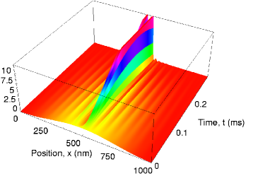
Figure 1: (Color online). Time evolution of the controlled wave packet density $|\Psi(x,t)|^{2}$ in an infinite rectangular well. Note monotonic increase of the wave packet height and decrease of its width.

As we mentioned above, it is easy to show that the matrix element $d_{j1}=<\psi_{k}|U_{in}|\psi_{1}>=-4L(\cos(\pi j)j+j)/(\pi^{2}(1-2j^{2}+j^{4}))$, so $d_{j1}=0$, if $j$ is odd, and $d_{j1}\neq 0$ if $j$ is even. We assume the system initially is in the ground state, thus it is impossible to drive the system into a squeezed target state with the same symmetry in the long wavelength limit. In order to utilize the only allowed ground state-odd states transitions, the target state $\Psi_{T}(x)$ is chosen to be an antisymmetric wave packet parameterized by $\sigma$ and located at position $x_{0}$:

$$\Psi_{T}(x)=B(x-x_{0})\exp(-(x-x_{0})^{2}/\sigma^{2}),$$ (12)

where the constant $B$ is determined from the normalization condition over the interval $[0,L]$. In the limit $\sigma\to 0$, $\Psi_{T}(x)$ becomes equivalent to the first derivative of the Dirac delta function $\delta^{\prime}(x-x_{0})$, and it has the minimum kinetic energy among all other wave packets with the same symmetry and given width $\sigma$. The amplitudes of the final state in the basis of the infinite well potential $a^{T}_{j}$ can be calculated analytically in terms of the Erf(x) function.

The ultimate goal of a useful squeezing algorithm is to create a wave packet with a characteristic size much less than the characteristic length scale of the inhomogeneous control potential. A possible realization of the proposed squeezing method in the long wave length limit is to control ions of charge $+q$ in the oscillating linear potentials. Let us assume for simplicity $q=|e|$. In a typical experiment let us assume the intensity of the highest mode of the controlling electromagnetic field is of the order of $100$ mW/cm², that corresponds to the electric field of $E=8.0\times 10^{-2}$V/m. We assume the initial width of the wave packet to be of the order of the infinite well trapping potential $L=1\times 10^{-6}$m, and the final width of the wave packet $\sigma\approx L/50=20$ nm. Using Eq.(11), we estimate duration of the squeezing procedure $T=\pi\hbar a_{30}^{T}/(Ed_{1\;30})\approx 3\times 10^{-4}$ s.

In Fig. 1 we show time evolution of the wave packet density $|\Psi(x,t)|^{2}$, trapped in the infinite well potential $x\in(0,L)$ under the control of the optimal field determined by Eq.(11). We choose $N=30$ of controlled levels, $x_{0}=L/2$, and final width $\sigma=L/50$. Note, that the height of the controlled wave packet is increasing monotonically, while the width is monotonically decreasing to its theoretical target limit. This is a direct consequence that the control is optimal, opposite to the previous studies (see, for example, Fig. 3 in optimal_squeezing , the non-monotonous decrease of the width of the wave packet is an indication that the numerical solution is a local extremum).

If it is more preferable to use neutral atoms instead of ions, then the necessary control potential can be created using dipole forces which are proportional to the amplitude gradient of the laser field cohen_tannuji . Note, that unlike in the case of ions, the dipole force arises for sufficiently inhomogeneous laser fields.

Another possible way to realize the proposed squeezing method is to consider control of molecular wave packets, or electron wave packets in artificial molecules: quantum dots. In this case one starts from the ground state and finishes at the linear combination of the vibrational (or eigenstates of the confining potential in the case of quantum dots) states, that builds up a narrow wave packet at a given time $T$. The latter can be probed by means of the ultrafast spectroscopy.

In this work we have derived analytically the control potential to localize an atomic wave packet in real space. This method is based on our knowledge of the eigenenergies and eigenfunctions of the controlled system in the trapping potential, and it is rigorous under the approximations made. Note, we can achieve the wave packet squeezing using control potentials with much larger wavelength ($\beta\to 0$) compare to the characteristic scale of the squeezed wave packet $\sigma$, that may be useful in atom lithography.

One essential assumption we made is a strong unharmonicity of the trapping potential. This assumption assures us that resonance frequencies between the initial (ground) state and multiple final states are all well separated. The trapping potential can be different from the infinite well potential considered in this work, but it will be more difficult to obtain solution in a simple analytical form. The presented method breaks down for relatively short control intervals $T$ or relatively strong control fields, when the RWA is not applicable. Another limitation is that the control interval cannot be very large, since the approximation that decoherence effects are negligible $T\gamma\ll 1$ should hold.

The resulting optimal control field has a complicated spectrum and shape, and it may be hard to obtain it using the standard numerical solution techniques for optimal control problems optimal_squeezing . That makes analytical form of the presented solutions even more attractive.

This work was carried out under the auspices of the National Nuclear Security Administration of the U.S. Department of Energy at Los Alamos National Laboratory under Contract No. DE-AC52-06NA25396.

References

- (1) I. Averbukh and M. Shapiro, Phys. Rev. A, 47, 5086 (1993).
- (2) Y. Ohtsuki, H. Kono, and Y. Fujimura, Chem. Phys. 109, 9318 (1998).
- (3) B. Y. Chang, S. Lee, I. R. Sola, J. Sanatmaria, J. Chem. Phys., 122, 204316 (2005).
- (4) G. Raithel, G. Birkl, W. D. Phillips, and S. L. Rolston, Phys. Rev. Lett. 78, 2928 (1997).
- (5) M. Leibscher and I. Sh. Averbukh, Phys. Rev. A, 65, 053816 (2002).
- (6) W. H. Oskay, D. A. Steck, and M. G. Raizen, Phys. Rev. Lett. 89, 283001 (2002).
- (7) L. E. E. de Araujo, I. A. Wamsley and C. R. Stroud, Jn. Phys. Rev. Lett. 81, 955 (1998); L. E. E. de Araujo and I. A. Wamsley, J. Phys. Chem. A, 103, 10409 (1999); L. E. E. de Araujo and I. A. Wamsley, Phys. Rev. A, 63, 023401 (2001).
- (8) C. J. Lee, Phys. Rev. A, 61, 063604 (2000).
- (9) J. L. Krause, M. Shapiro, and R. Bersohn, J. Chem. Phys. 94, 5499 (1991).
- (10) J. P. Gordon, A. Ashkin, Phys. Rev. A 61, 1606 (1980).
- (11) V. M. Akulin, N. V. Karlov, “Intence Resonant Interactions in Quantum Electronics”, Springer-Verlag, (1992).
- (12) M. E. Garcia and I. Grigorenko, J. Phys. B: At. Mol. Opt. Phys. 37 2569 (2004).
- (13) P. L. Knight, L. Allen, Phys. Rev A, 7, 368 (1973).
- (14) F. M. Fernandez, Phys. Rev A, 67, 022104 (2003).