Superconductivity in Multilayer Perovskite: Weak Coupling Analysis

Abstract

We investigate the superconductivity of a three-dimensional d-p model with a multilayer perovskite structure on the basis of the second-order perturabation theory within the weak coupling framework. Our model has been designed with multilayer high-$T_{\mathrm{c}}$ superconducting cuprates in mind. In our model, multiple Fermi surfaces appear, and the component of a superconducting gap function develops on each band. We have found that the multilayer structure can stabilize the superconductivity in a wide doping range.

1 Introduction

In the last decade, high-$T_{\mathrm{c}}$ superconducting cuprates (HTSCs) with multilayer structure have been investigated extensively by various experimental methods [1, 2, 3]. Multilayer cuprates typically have higher $T_{\mathrm{c}}$ than single-layer ones. The nuclear magnetic resonance (NMR) measurement systematically reveals the local hole concentration on each layer of the multilayer HTSCs. In previous excellent studies [4, 5], each layer has been crystallographically classified into an outer or inner CuO₂ plane in a unit cell. The authors found the relationship between the difference in the local hole concentration among these two types of planes and $T_{\mathrm{c}}$, and they considered the condition in which $T_{\mathrm{c}}$ can be maximized. The results suggest that multiple Fermi surfaces are involved in superconductivity, and that an extensive theory on multilayer materials should be constructed on the basis of the model with multibands.

The above NMR study mainly revealed the characteristic of the multilayer compounds for $n\geq 3$, where $n$ is the number of CuO₂ planes per unit cell. The characteristic feature of multiband systems can also appear explicitly in a bilayer compound. In Bi₂Sr₂CaCu₂O_8+δ (Bi2212), which is another typical bilayer material, the high-resolution angle-resolved-photoemission spectroscopy (ARPES) successfully revealed the doubling of a band near the Fermi level [6, 7]. This splitting is negligible along the $(0,0)\rightarrow(\pi,\pi)$ nodal line and maximum at $(\pi,0)$ in momentum space. This momentum dependence of energy splitting is qualitatively consistent with the LDA prediction for YBa₂Cu₃O₇ [8], which is another bilayer material. This LDA calculation predicted that a Cu $4s$ orbital has a transfer integral between that in the other layer. This interlayer coupling causes a single band to split into antibonding and bonding bands.

A multilayer model has been theoretically studied since the early 1990s by fluctuation exchange (FLEX) approximation [9] and by quantum Monte Carlo (QMC) simulation [9, 10] on the basis of the two-dimensional (2D) multilayer Hubbard model. These studies have shown that the $d_{x^{2}-y^{2}}$-wave pairing correlations are reduced by interlayer transfer, which is independent of the in-plane momenta, $k_{x}$ and $k_{y}$. However, when we introduce interlayer transfer into our model, it is important to consider the symmetry of interlayer transfer integrals in which Cu $4s$ electrons participate. Liechtenstein et al. considered this point and studied the extended Hubbard model with anisotropic interlayer hopping, using the FLEX approximation [11]. Although they could not reproduce the experimental result of bilayer materials having higher $T_{\mathrm{c}}$ than single-layer ones, their work should be appreciated as the first theoretical analysis of the superconductivity of realistic multilayer systems. All the theoretical works have been done on the basis of the 2D model Hamiltonian. We feel that we should investigate the three-dimensional model Hamiltonian with anisotropic interlayer hopping to estimate $T_{\mathrm{c}}$ of multilayer materials.

In this study, we investigate the superconductivity of multilayer perovskite. We adopt the three-dimensional (3D) d-p model with anisotropic interlayer transfers as our model Hamiltonian. In our model, we introduce such a small on-site Coulomb interaction that the second-order perturbation theory (SOPT) can be justified. We can treat the superconductivity within the weak coupling analysis because, in our model, the effective interaction for Cooper pairing is so small that only the electrons on the Fermi surface are involved in the superconductivity. The weak coupling formalism for the repulsive interaction model, since the pioneering work by Kohn and Luttinger [12], has been developed by many theorists  [13, 14, 15, 16, 17]. Recently, this formalism was applied, by Kondo, to the 2D Hubbard model with the formulation applicable even for the case with a very small effective interaction [18]. We apply Kondo’s formulation to our model with multiple Fermi surfaces, and clarify how the superconducting gap depends on $n$ of layers. We can show that the calculation on the basis of 3D model Hamiltonian is requisite for the true estimation of $T_{\mathrm{c}}$ of multilayer materials. Our obtained results are not only to be compared with the actual $T_{\mathrm{c}}$ of multilayer materials but to be considered as a guide for designing materials with high $T_{\mathrm{c}}$.

2 Formulation

We can decompose our 3D d-p model with the $n$-layer perovskite structure into several parts as follows:

$$H=\sum_{l=1}^{n} \left[\right.H_{l}^{0}+H_{l+1,\,l}^{0}+H_{l}^{\prime}$$

$$-\mu\sum_{\mib{k}\sigma}(d_{\mib{k}\,l\sigma}^{\dagger}d_{\mib{k}\,l\sigma}+p_{\mib{k}\,l\sigma}^{x\dagger}p_{\mib{k}\,l\sigma}^{x}+p_{\mib{k}\,l\sigma}^{y\dagger}p_{\mib{k}\,l\sigma}^{y})\left.\right]$$

(1)

where $d_{\mib{k}\,l\sigma}$ $(d_{\mib{k}\,l\sigma}^{\dagger})$, $p_{\mib{k}\,l\sigma}^{x}$ $(p_{\mib{k}\,l\sigma}^{x\dagger})$ and $p_{\mib{k}\,l\sigma}^{y}$ $(p_{\mib{k}\,l\sigma}^{y\dagger})$ are the annihilation (creation) operators for d-, p^x- and p^y-electrons of momentum $\mib{k}$ and spin $\sigma=\{\uparrow,\downarrow\}$ on the $l$-th layer, respectively. We define $n+1\equiv 1$, and the chemical potential is represented by $\mu$. The noninteracting parts in eq. (1), i.e., $H_{l}^{0}$ and $H_{l+1,\,l}^{0}$ , are represented by

$$H_{l}^{0}$$

$$= \sum_{\mib{k}\sigma}\left(d_{\mib{k}\,l\sigma}^{\dagger}\,p_{\mib{k}\,l\sigma}^{x\dagger}\,p_{\mib{k}\,l\sigma}^{y\dagger}\right)\left(\begin{array}[]{ccc}\Delta_{l}&\zeta_{\mib{k}}^{x}&\zeta_{\mib{k}}^{y}\\ -\zeta_{\mib{k}}^{x}&0&\zeta_{\mib{k}}^{p}\\ -\zeta_{\mib{k}}^{y}&\zeta_{\mib{k}}^{p}&0\\ \end{array}\right)\left(\begin{array}[]{c}d_{\mib{k}\,l\sigma}\\ p_{\mib{k}\,l\sigma}^{x}\\ p_{\mib{k}\,l\sigma}^{y}\\ \end{array}\right)$$ (8)

and

$$H_{l+1,\,l}^{0}=\left\{\begin{array}[]{ll}\sum_{\mib{k}\sigma}\zeta_{\mib{k}}^{z}\,d_{\mib{k}\,l+1\sigma}^{\dagger}d_{\mib{k}\,l\sigma}+{\mathrm{h.c.}}&l=n\\ \sum_{\mib{k}\sigma}\zeta_{\mib{k}}^{d}\,d_{\mib{k}\,l+1\sigma}^{\dagger}d_{\mib{k}\,l\sigma}+{\mathrm{h.c.}}&l<n\end{array}\right..$$ (12)

In eqs. (LABEL:eq:8) and (12) we take the lattice constant of the square lattice formed of Cu sites, $a$, as the unit length. Using it, we can represent $\zeta_{\mib{k}}^{p}=4t_{pp}\sin\frac{k_{x}}{2}\sin\frac{k_{y}}{2}$, $\zeta_{\mib{k}}^{x}=2{\rm i}t_{dp}\sin\frac{k_{x}}{2}$, $\zeta_{\mib{k}}^{y}=2{\rm i}t_{dp}\sin\frac{k_{y}}{2}$, $\zeta_{\mib{k}}^{z}=t_{\perp}\cos\frac{k_{x}}{2}\cos\frac{k_{y}}{2}e^{{\mathrm{i}}k_{z}r_{a}}$, and $\zeta_{\mib{k}}^{d}=\frac{t_{dd}}{4}(\cos k_{x}-\cos k_{y})^{2}e^{{\mathrm{i}}k_{z}r_{b}}$, where $r_{a}=\frac{c_{a}}{c_{a}+(n-1)c_{b}}$ and $r_{b}=\frac{c_{b}}{c_{a}+(n-1)c_{b}}$. $c_{a}$ and $c_{b}$ represent the distances among CuO₂ planes, as shown in Fig. 1. Hereafter, we use ’IP’ and ’OP’ as abbreviations for inner CuO₂ planes ($1<l<n$) and outer CuO₂ planes ($l=1\mbox{ or }n$), respectively. $\Delta_{l}$ is the hybridization gap energy on the $l$-th layer between d- and p-orbitals. When $n\geq 3$, our model has several crystallographically inhomogeneous CuO₂ planes, and $\Delta_{l}$ varies according to $l$. We can define $\Delta_{l}$ as

$$\Delta_{l}=\left\{\begin{array}[]{ll}\Delta_{dp}&l=1\mbox{ or }n\\ \Delta_{dp}-\frac{\alpha}{r_{a}}&1<l<n\end{array}\right.,$$ (15)

where $\alpha$ is the constant chosen so as to reproduce the difference in doped carriers between OP and IP.

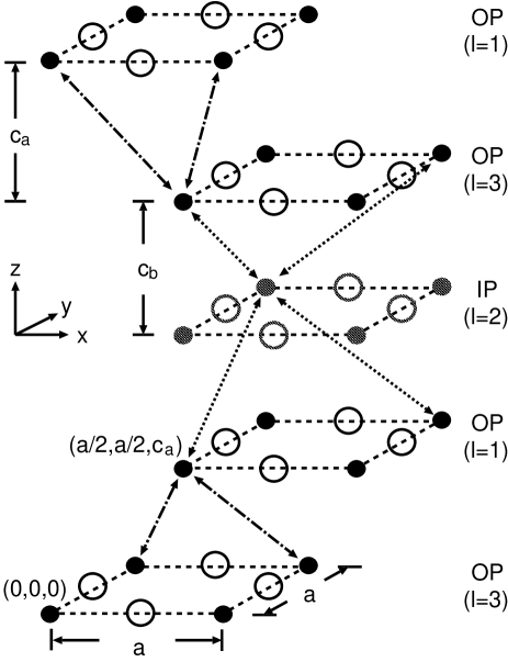
Figure 1: Crystal structure modeled after trilayered perovskite. Filled (Open) circles represent copper (oxygen) cites. Dotted (Dot-dashed) arrows conecting copper cites correspond to $\zeta_{\mib{k}}^{d}$ ($\zeta_{\mib{k}}^{z}$) in the text.

We consider only the on-site Coulomb repulsion among d-electrons. Thus, the interacting part $H_{l}^{\prime}$ in eq. (1) is described as

$$H_{l}^{\prime}=\frac{U}{N}\sum_{\mib{k}\mib{k}^{\prime}\mib{q}}d_{\mib{k}+\mib{q}\,l\uparrow}^{\dagger}d_{\mib{k}^{\prime}-\mib{q}\,l\downarrow}^{\dagger}d_{\mib{k}^{\prime}\,l\downarrow}d_{\mib{k}\,l\uparrow}.$$ (16)

In eq. (16), $N$ is the number of $\mib{k}$-space lattice points in the first Brillouin zone (FBZ), which is equal to the number of Cu sites in the real space.

In the following part, we assume that only the electrons on the Fermi surface of the same band can have singlet pair instability. For our $n$-layer model, $n$ d-like bands always intersect with the Fermi level. Thus, according to the BCS theory, we have the following self-consistent equation for the pair function on the $\lambda$-th d-like band, $\Phi_{\mib{k}\lambda}$:

$$\Phi_{\mib{k}\lambda}=-\frac{1}{2N}\!\sum_{ij\mib{k}^{\prime}\nu}V_{ij}(\mib{k}+\mib{k}^{\prime})\frac{z_{i\lambda}(\mib{k})z_{j\nu}(\mib{k}^{\prime})}{\sqrt{\left(\varepsilon_{\mib{k}^{\prime}\nu}-\mu\right)^{2}+\left(\Phi_{\mib{k}^{\prime}\nu}\right)^{2}}}\,\Phi_{\mib{k}^{\prime}\nu},$$ (17)

where $i,j=1,\ldots,n$ (layer indices) and $\lambda,\nu=1,\ldots,n$ (d-like band indices). $V_{ij}(\mib{q})$ represents the effective singlet pair scattering between a d-electron on the $i$-th layer and one on the $j$-th layer. $\varepsilon_{\mib{k}\nu}$ represents the energy dispersion of the $\nu$-th d-like band, and $z_{i\lambda}(\mib{k})$ represents the matrix element of unitary transformation. They are obtained by solving the eigenequation for the noninteracting part in eq. (1). We set $\Phi_{\mib{k}\lambda}=\Delta_{\mathrm{sc}}\!\cdot\!\Psi_{\mib{k}\lambda}$, where $\Delta_{\mathrm{sc}}$ denotes the magnitude of $\Phi_{\mib{k}\lambda}$ and $\Psi_{\mib{k}\lambda}$ represents its $\mib{k}$-dependence on the $\lambda$-th d-like band. On the basis of Kondo’s argument, [18] retaining only the divergent term, we can rewrite eq. (17) as

$$\begin{split}\Psi_{\mib{k}\lambda}&=\\ &\log_{e}\Delta_{\mathrm{sc}}\cdot\frac{1}{N}\sum_{ij\mib{k}^{\prime}\nu}V_{ij}(\mib{k}+\mib{k}^{\prime})z_{i\lambda}(\mib{k})z_{j\nu}(\mib{k}^{\prime})\delta(\varepsilon_{\mib{k}^{\prime}\nu}-\mu)\Psi_{\mib{k}^{\prime}\nu}\end{split}$$ (18)

for very small $\Delta_{\mathrm{sc}}$. Equation (18) is a homogeneous integral equation for $\Psi_{\mib{k}\lambda}$ with the eigenvalue of $1/\log\Delta_{\mathrm{sc}}$. We are interested in obtaining the most stable superconducting state, thus we must find the eigenvector $\Psi_{\mib{k}\lambda}$ with the smallest eigenvalue $1/\log\Delta_{\mathrm{sc}}$ using eq. (18) when $\Delta_{\mathrm{sc}}$ is maximum. In our previous paper, we confirmed that the most stable pairing state near half-filling is the $d_{x^{2}-y^{2}}$-wave, by a similar approach based on 2D d-p model [19]. Hence, when we assume that

$$\Psi_{\mib{k}\lambda}=a_{\lambda}(k_{z})(\cos k_{x}-\cos k_{y}),$$ (19)

we can safely reduce our original eigenvalue problem for $\Psi_{\mib{k}\lambda}$ to an eigenvalue problem for $a_{\lambda}(k_{z})$ in order to seek only the most stable pairing state. Furthermore, considering the symmetry of $\Psi_{\mib{k}\lambda}$ in eq. (19), we can take

$$\begin{split}V_{ij}(\mib{q})&=U^{2}\chi_{ij}(\mib{q})\\ &=\frac{U^{2}}{N}\sum_{\mib{k}\xi\eta}z_{i\xi}(\mib{q}+\mib{k})z_{j\eta}(\mib{k})\frac{\left(1-f_{\mib{q}+\mib{k}\xi}\right)f_{\mib{k}\eta}}{\varepsilon_{\mib{q}+\mib{k}\xi}-\varepsilon_{\mib{k}\eta}}\end{split}$$ (20)

within SOPT. In eq. (20),

$$f_{\mib{k}\eta}=\frac{1}{2}\left[1-\tanh\left(\frac{\varepsilon_{\mib{k}\eta}-\mu}{2T}\right)\right],$$ (21)

and $T$ denotes the temperature.

3 Results and Discussion

In our present analyses, all $\varepsilon_{\mib{k}\nu}$ and $z_{i\lambda}(\mib{k})$ in eq. (18) are first calculated for $64^{3}$ $\mib{k}-$points on an equally spaced mesh in FBZ for each band. Then, we calculate $V_{ij}(\mib{k}+\mib{k}^{\prime})$ in eq. (18) only for $\mib{k}-$ and $\mib{k}^{\prime}-$points satisfying the conditions $\varepsilon_{\mib{k}\lambda}=\mu$ and $\varepsilon_{\mib{k}^{\prime}\nu}=\mu$, respectively. When we calculate $V_{ij}(\mib{k}+\mib{k}^{\prime})$ according to eqs. (20) and (21), we set the temperature $T=0.001\,$eV$\sim 10\,$K, at which our system can be considered to behave similarly to that in the ground state. These calculations have been performed at $U=0.5\,$eV, where magnetic instabilities cannot occur. We take $c_{a}=0.3$ and $c_{b}=0.7$ for all $n$. Other common parameters are summarized in Table 1.

$t_{dp}$	$t_{pp}$	$t_{dd}$	$t_{\perp}$	$\Delta_{dp}$
$1.00\,$eV	$-300\,$meV	$10\,$meV	$5\,$meV	$2.10\,$eV

Table 1: Transfer and hybridization gap energies.

In order to solve eq. (18) practically, we substitute $\Psi$ into both sides of eq. (18) using eq. (19) and integrate for $k_{x}$, $k_{x}^{\prime}$, $k_{y}$, and $k_{y}^{\prime}$. Thus, we reduce eq. (18) to the eigenequation for $a_{\lambda}(k_{z})$. When we solve it numerically by the standard method, we can finally obtain both the eigenvalue, $1/\log_{e}\Delta_{\mathrm{sc}}$, and the eigenvector, $a_{\lambda}(k_{z})$.

First, we summarize our results on $\Delta_{\mathrm{sc}}$ vs $\delta_{\mathrm{h}}$($\delta_{\mathrm{e}}$) in Fig. 2. As discussed in our previous paper on the two-dimensional (2D) d-p model [19], the existence of a Van Hove singularity (VHS) at the Fermi level causes a high density of states (DOS) and enhances $\Delta_{\mathrm{sc}}$. In the 2D d-p model the parts of the Fermi surface with VHS are distributed as lines. Therefore $\Delta_{\mathrm{sc}}$ varies drastically in the neighborhood of the doping point at which the Fermi surface has VHS. This is in contrast with the case in the 3D d-p model. Although the energy dispersion along the $c$-axis introduced in our analyses is very weak, as indicated in Table 1, the parts of the Fermi surface with VHS are distributed as points. Thus, the transition of $\Delta_{\mathrm{sc}}$ in the 3D model is milder than that in the 2D model, as seen in Fig. 2.

Furthermore, in Fig. 2 we can clearly recognize that the enhanced $\Delta_{\mathrm{sc}}$ prevails in a wider doping region with larger $n$. This result is caused by the multilayering effect introduced as described by eq. (15). In order to explain how the multilayering effect occurs, we show the eigensolutions, $a_{\lambda}(k_{z})$, defined by eq.(19), and the Fermi surfaces for the cases with $n=3,4,$ and $5$ in Figs. 3, 4, and 5, respectively.

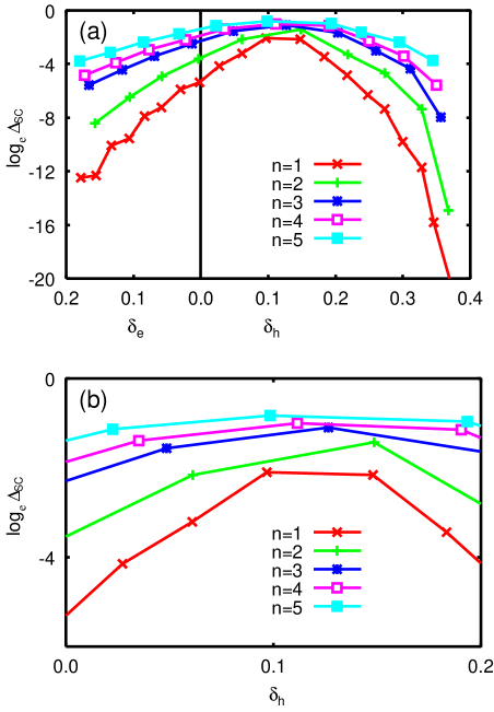
Figure 2: (a) $\log\Delta_{\mathrm{sc}}$ vs $\delta_{\mathrm{h}}$ (hole-doped) or $\delta_{\mathrm{e}}$ (electron-doped) in the cases of $n=1,2,3,4,$ and $5$. (b) Magnification of (a) in the region of $0.0\leq\delta_{\mathrm{h}}\leq 0.2$.

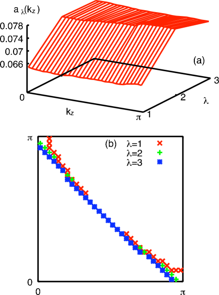
Figure 3: The results for $n=3$ and $\delta_{\mathrm{h}}=0.127$. (a) The eigensolution $a_{\lambda}(k_{z})$. (b) The Fermi surface projected onto the plane with $k_{z}=0$.

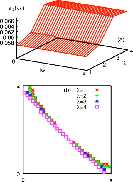
Figure 4: The results for $n=4$ and $\delta_{\mathrm{h}}=0.112$. (a) The eigensolution $a_{\lambda}(k_{z})$. (b) The Fermi surface projected onto the plane with $k_{z}=0$.

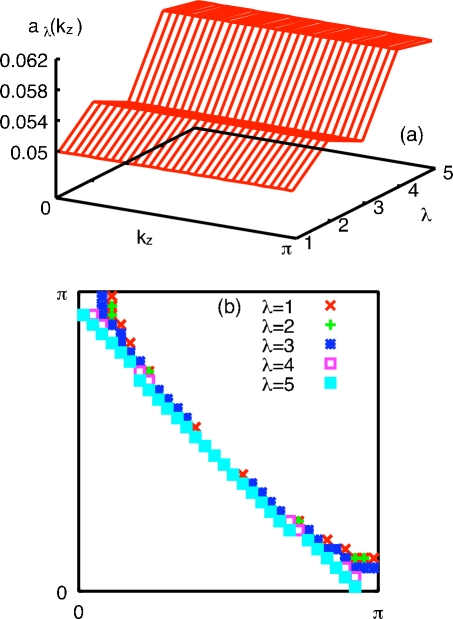
Figure 5: The results for $n=5$ and $\delta_{\mathrm{h}}=0.098$. (a) The eigensolution $a_{\lambda}(k_{z})$. (b) The Fermi surface projected onto the plane with $k_{z}=0$.

In Fig. 3 the highest amplitude of the eigensolution appears in the band with $\lambda=2$, whose Fermi surface most closely approaches the VHS points, i.e., $(\pm\pi,0,[-\pi,\pi])$ and $(0,\pm\pi,[-\pi,\pi])$. Thus, the band with $\lambda=2$ has the largest DOS near VHS points and is dominant in the superconductivity. For the same reason, the largest amplitude of the eigensolution appears in the band with $\lambda=3$ and in the one with $\lambda=4$, as shown in Figs. 4 and 5, respectively.

When we change the amount of doped carriers, the Fermi surface should be transformed. As a result, another band could then have the largest DOS near the VHS points and dominate the superconductivity. This possibility should be further increased more if our model has more alternative bands. Hence, the enhanced $\Delta_{\mathrm{sc}}$ tends to prevail in a wider doping region with larger $n$. This tendency should remain when $n$ becomes much larger, as long as the conventional Fermi surface can be defined. However, the largest value of $\Delta_{\mathrm{sc}}$ should be saturated toward the intrinsic value for $n\rightarrow\infty$.

Hereafter, we turn our attention to the maximum $T_{\mathrm{c}}$ of the $n$-layered materials, which would be proportional to the maximum $\Delta_{\mathrm{sc}}$ in our calculated results. In several real materials, the largest $T_{\mathrm{c}}$ is achieved when $n=3$ or $n=4$, and $T_{\mathrm{c}}$ is rather low when $n=5$ [4, 5]. For such materials our assumption that the well-defined Fermi surface exists might not be valid. For example, in the five-layered compound HgBa₂Ca₄Cu₅O_y, the inner CuO₂ planes turn out to be antiferromagnetic on account of the strong electronic correlation [20]. Concerning the strong electronic correlation, other theoretical works based on the 2D multilayer t-J model have been extensively carried out by Mori et al. [21, 22]. Their approach would be better for explaining the results for such compounds.

Although our results on $T_{\mathrm{c}}$ are not consistent with those for several real materials, our conclusion on the multilayering effect is clearly applicable to other real materials. Indeed, (Cu,C)Ba₂Ca₃Cu₄O_12+y (Cu1234), has a high $T_{\mathrm{c}}$ even though it is in the heavily overdoped region [1, 3, 2]. Cu1234 has been revealed, by NMR experiment, to have doped holes that are almost uniformly distributed into each layer [4, 5]. Thus, our assumption concerning the Fermi surface is considered to be valid for Cu1234.

4 Summary

We demonstrated that the ground state of the 3D d-p model with a multilayer perovskite structure can be in the $d_{x^{2}-y^{2}}$-wave superconducting state up to the second-order in the perturbation theory framework. In the multilayer system, the region with large $\log\Delta_{\mathrm{sc}}$ can expand further. This is caused by the multilayering effect, which can increase the chance that the Fermi surface has VHS and can maintain a high DOS around the Fermi level over a wide doping region. This multilayering effect works very well when the unit cell contains more layers, as long as a well-defined Fermi surface exists.

References

- [1] H. Ihara, A. Iyo, K. Ishida, N. Terada, M. Tokumoto, Y. Sekita, M. Umeda, K. Tanaka, K. Tokiwa, T. Tsukamoto and T. Watanabe: Physica C 282-287 (1997) 1973.
- [2] T. Watanabe, S. Miyashita, N. Ichioka, K. Tokiwa, K. Tanaka, A. Iyo, Y. Tanaka and H. Ihara: Physica B 284-288 (2000) 1075.
- [3] H. Ihara, A. Iyo, Y. Tanaka, N. Terada, K. Tokiwa, T. Watanabe, Y. Tokunaga, K. Ishida, Y. Kitaoka and N. Hamada: Physica B 292 (2000) 238.
- [4] Y. Tokunaga, K. Ishida, Y. Kitaoka, K. Asayama, K. Tokiwa, A. Iyo and H. Ihara: Phys. Rev. B 61 (2000) 9707.
- [5] H. Kotegawa, Y. Tokunaga, K. Ishida, G.-q. Zheng, Y. Kitaoka, H. Kito, A. Iyo, K. Tokiwa, T. Watanabe and H. Ihara: Phys. Rev. B 64 (2001) 064515.
- [6] Y.-D. Chuang, A. D. Gromko, A. Fedorov, Y. Aiura, K. Oka, Yoichi Ando, H. Eisaki, S. I. Uchida and D. S. Dessau: Phys. Rev. Lett. 87 (2001) 117002.
- [7] D. L. Feng, N. P. Armitage, D. H. Lu, A. Damascelli, J. P. Hu, P. Bogdanov, A. Lanzara, F. Ronning, K. M. Shen, H. Eisaki, C. Kim, Z.-X. Shen, J.-i. Shimoyama and K. Kishio: Phys. Rev. Lett. 86 (2001) 5550.
- [8] O. K. Andersen, A. I. Liechtenstein, O. Jepsen and F. Paulsen: J. Phys. Chem. Solids 56 (1995) 1573.
- [9] N. Bulut, D. J. Scalapino and R. T. Scalettar: Phys. Rev. B 45 (1992) 5577.
- [10] R. T. Scalettar, J. W. Cannon, D. J. Scalapino and R. L. Sugar: Phys. Rev. B 50 (1994) 13419.
- [11] A. I. Liechtenstein, O. Gunnarsson, O. K. Andersen and R. M. Martin: Phys. Rev. B 54 (1996) 12505.
- [12] W. Kohn and J. M. Luttinger: Phys. Rev. Lett. 15 (1965) 524.
- [13] D. Fay and A. Layzer: Phys. Rev. Lett. 20 (1968) 187.
- [14] S. Nakajima: Prog. Theor. Phys. 50 (1973) 1101.
- [15] P. W. Anderson and W. F. Brinkman: Phys. Rev. Lett. 30 (1973) 1108.
- [16] M. Yu. Kagan and A. V. Chubukov: JETP Lett. 47 (1988) 614.
- [17] R. Hlubina: Phys. Rev. B 59 (1999) 9600.
- [18] J. Kondo: J. Phys. Soc. Jpn. 70 (2001) 808.
- [19] S. Koikegami and T. Yanagisawa: J. Phys. Soc. Jpn. 70 (2001) 3499; 71 (2002) 671(E).
- [20] H. Kotegawa, Y. Tokunaga, Y. Araki, G.-q. Zheng, Y. Kitaoka, K. Tokiwa, K. Ito, T. Watanabe, A. Iyo, Y. Tanaka and H. Ihara: Phys. Rev. B 69 (2004) 014501.
- [21] M. Mori, T. Tohyama and S. Maekawa: Phys. Rev. B 66 (2002) 064502.
- [22] M. Mori, T. Tohyama and S. Maekawa: Physica C 388 (2003) 51; 392-396 (2003) 123; 378 (2002) 333.