Radio source calibration for the VSA and other CMB instruments at around GHz
Abstract
Accurate calibration of data is essential for the current generation of CMB experiments. Using data from the Very Small Array (VSA), we describe procedures which will lead to an accuracy of 1 percent or better for experiments such as the VSA and CBI. Particular attention is paid to the stability of the receiver systems, the quality of the site and frequent observations of reference sources. At 30 GHz the careful correction for atmospheric emission and absorption is shown to be essential for achieving 1 percent precision.
The sources for which a 1 percent relative flux density calibration was achieved included Cas A, Cyg A, Tau A and NGC7027 and the planets Venus, Jupiter and Saturn. A flux density, or brightness temperature in the case of the planets, was derived at 33 GHz relative to Jupiter which was adopted as the fundamental calibrator. A spectral index at GHz is given for each.
Cas A,Tau A, NGC7027 and Venus were examined for variability. Cas A was found to be decreasing at percent per year over the period March 2001 to August 2004. In the same period Tau A was decreasing at percent per year. A survey of the published data showed that the planetary nebula NGC7027 decreased at percent per year over the period 1967 to 2003. Venus showed an insignificant ( percent) variation with Venusian illumination. The integrated polarization of Tau A at 33 GHz was found to be percent at pa .
keywords:
cosmology: observations – cosmic microwave background – techniques: interferometric – methods: observational – radio continuum: Solar system – radio continuum: ISM1 Introduction
With the increasing sensitivity of CMB experiments, it is important to have accurate calibration of the intensity or temperature scale of each experiment. The cosmological significance of the data is directly dependent on this scale. For example, the amplitude of the first peak in the CMB power spectrum is proportional to while the ratio of the first to the third peak, derived from a mix of experiments probing different angular modes , is also sensitive to . Furthermore, the fractional uncertainty in the power spectrum is twice that of the fractional uncertainty in the temperature scale. Current CMB experiments would greatly benefit from a coherent calibration across experiments such as Planck, WMAP, CBI, VSA etc. at an accuracy of % or better. The present investigation provides a set of source intensities calibrated to this precision at a frequency of 33 GHz.
We have chosen the brightest planets and strongest radio sources to calibrate the VSA on a frequent (typically few hours) basis during CMB observations. The basic calibration of all the targets used in the VSA is in terms of an assumed brightness temperature of Jupiter (Watson et al. 2003; Dickinson et al. 2004), which in turn, is tied to the CMB dipole (Hinshaw et al. 2008).
Inevitably the strongest sources used for the frequent calibration of VSA data are sufficiently extended (a few arcmin) that their total flux densities require correction when applied to the 10 arcmin resolution of the VSA at an accuracy of better than 1%. Cas A, Tau A and Cyg A fall into this category although for Cyg A the effect is 0.3. The planets do not require such a correction.
The polarization of the calibrators also needs to be taken into account. The most strongly polarized source is Tau A. The integrated emission from HII regions and the planets are not expected to be polarized. The radial polarization of the planets would only be of concern if there were a significant phase effect in the brightness distribution across the planet.
Time variability is an important consideration when using calibrators. Many of the stronger extragalactic sources such as quasars have to be rejected for this reason. This is an integral part of the present study.
The spectral index of a calibrator needs to be specified if the calibration process is to be useful between experiments which have different central frequencies and bandwidths even within the 1 cm wavelength band investigated here. In general, spectral index data are taken from the literature.
The main challenge in accurate calibration of ground-based observations at centimetric and millimetric frequencies is provided by the atmosphere. A high dry site is a prerequisite. The Izaña observatory of the IAC has a proven record of observations in the range 10-33 GHz (Davies et al. 1996). An assessment of its properties at these frequencies will be given in a separate paper (Davies et al., in prep.).
This paper is arranged as follows. Section 2 describes the relevant features of the VSA used in this investigation. The philosophy of the approach, including the method of determining the atmospheric corrections, are given in Section 3. The results given as flux densities, or brightness temperatures in the case of the planets, are presented along with the adopted spectral indices in Section 4, which also includes a discussion of source variability and polarization. The conclusions of this work are summarised in Section 5.
2 The VSA and its calibration system
The advantage of using an interferometer for “point source” flux density measurements is that the extended emission from the sky, atmosphere and the ground can be largely eliminated. The VSA is described in detail by Watson et al. (2003), Scott et al. (2003) and Dickinson et al. (2004). A summary of its main features is now given.
2.1 The overall system
The Very Small Array (VSA) is a 14-element interferometer operating in the Ka band (26-36 GHz). It is located on the high and dry site at the Teide Observatory, Izaña, Tenerife at an altitude of 2340m. The antenna of each element consists of a conical corrugated horn feeding a paraboloidal mirror. Each antenna and its associated cryogenically cooled receiver system can be placed anywhere on a 4-m x 3-m tip-tilt table located in a metal enclosure to minimise any emission contribution from the ground. Due to the geometry of the table and the enclosure, the VSA declination is restricted to the range to . Tracking of a field is accomplished by a combination of table tilt and rotation of each mirror.
Since the beginning of CMB observations in September 2000 the VSA has been operated in both a compact and extended configuration. In the compact configuration the mirror diameters were 143mm giving a primary beamwidth (FWHP) of 46. The geometrical arrangement of the antennas on the table gave interferometer baseline lengths ranging from 0.20m to 1.23m allowing angular multipoles of l = 150 to 900 to be probed at the observing frequency of 34.1 GHz. The resolution of the array was arcmin depending on the field declination and hour angle range observed.
The extended array, which became operational in October 2001, used an antenna configuration which covered a baseline range of 0.6m to 2.5m thereby extending the range of angular multipoles to l = 1500 and gave a synthesized beamwidth (FWHP) of arcmin. The larger mirror diameters provided a factor of 1.6 improvement in filling factor and an overall factor of in temperature sensitivity (see Table 1). Since September 2005 the VSA has operated in a third configuration, the super-extended array, with 60 cm aperture mirrors (Genova-Santos et al. 2008).
The VSA has operated at either 33 or 34.1 GHz with an instantaneous bandwidth of 1.5 GHz. With an average system temperature of some K the VSA achieves an overall instantaneous point source sensitivity of and Jy s in the compact and extended configurations respectively; the corresponding temperature sensitivities are 40 and 15 mK s1/2. The VSA is linearly polarized in the vertical direction and is therefore sensitive to any linear polarization in the calibration sources.
2.2 Present analysis
An interferometer array like the VSA requires an accurate determination of the position of the antennas to produce reliable relative observations at the 1% level aimed at in this paper. A maximum likelihood technique has been applied to the calibrator source observations in order to constrain such telescope parameters as the antenna positions, effective observing frequencies and correlator amplitudes and phase shifts (Maisinger et al. 2003). The stability of the VSA is such that these calibration observations are required only every few hours.
The overall gain of each antenna is monitored continuously by means of a noise injection system. A modulated noise signal is injected into each antenna via a probe in the horn and is measured using phase-sensitive detection after the automatic gain control (AGC) stage in the IF system. The relative contribution of the constant noise source to the total output power from each antenna varies inversely with system temperature and thus a correction can be made to the overall flux calibration. This system allows account to be taken of the gain and variations in total set noise due, for example, to atmospheric emission. It potentially provides an indication of weather conditions and is a primary indicator for flagging weather-affected data in CMB observations. In the face of the stringent requirements here of better than 1% calibration accuracy, this approach had to be modified as described in the next section.
| Compact | Extended | |
|---|---|---|
| Declination range | to | to |
| Number of antennas (baselines) | 14(91) | 14(91) |
| Range of baseline lengths | 0.20 m to 1.23 m | 0.6 m to 2.5 m |
| Centre frequencies | 34 GHz | 33, 34 GHz |
| Bandwidth of observation | 1.5 GHz | 1.5 GHz |
| System temperature, Tsys | K | K |
| Mirror diameters | 143 mm | 332 mm |
| Primary beam (FWHM) | 4.6 | 2.0 |
| Synthesized beam (FWHM) | arcmin | arcmin |
| Range of angular multipole (l) | 150 to 900 | 300 to 1500 |
| Point source sensitivity | Jy s1/2 | Jy s1/2 |
| Temperature sensitivity per beam | mKs1/2 | mKs1/2 |
| Polarization | linear (vertical) | linear (vertical) |
3 The source calibration programme
We consider here the methods used to measure relative flux densities to an accuracy of 1 percent or better at a frequencies around 30 GHz.
3.1 Calibration sources for CMB observations
The sources available for this study are those bright enough to be detected with good signal to noise in say minutes of observing time. This limits them to 10 Jy in the two configurations, which allows the following sources to be used as primary calibrators: Tau A, Cas A, Cyg A, Jupiter, Saturn and Venus. Observations on these sources of 10-30 minutes are interleaved within CMB fields. These observations provide the data archive on which the present investigation is based. Additional long-track observations covering 3 hr in hour angle were used to quantify elevation-dependent atmospheric effects.
3.2 Data reduction procedures
The basic data reduction of VSA data followed the same procedure as described in early VSA work (e.g. Taylor et al. 2003; Dickinson et al. 2004). One radio source (or the CMB) is calibrated against another (the “ calibrator ”) by converting the units of the 91 raw visibilities from correlator units to to flux densities via the primary “ calibrator ” for each baseline and then combining them to give a mean flux density for the source. The resulting 91 baseline visibility tracks are checked by eye and interactively searched for residual contaminating signals. Due to the large number of calibrator observations we were able to be fastidious about data quality. Some 20% of the data are removed in this way in addition to the more obvious errors due to hardware failure and bad weather. The elevation of each source was recorded and could be used to make subsequent corrections for atmospheric effects.
3.3 Choice of fundamental reference source
The flux calibration of VSA data is tied to observations of Jupiter which is widely used as a calibrator for CMB observations in the range 10-500 GHz. Our early VSA results (see e.g. Scott et al. 2003; Taylor et al. 2003) were based on a brightness temperature TJ = 1525 K at 32 GHz, extrapolated to 33/34.1 GHz using , from direct measurements (Mason et al. 1999). The VSA calibration is now expressed in terms of the WMAP spectrum of Jupiter which is tied to the CMB dipole temperature. At 33 GHz, the most recent WMAP value is TJ = 146.60.75 K (Hill et al. 2008).111It is of interest to note that the previous WMAP value (Page et al. 2003) is identical to the new one (Hill et al. 2008) but with a larger error ( K) due to beam uncertainties. This led the CBI group (Readhead et al. 2004) to use a weighted estimate between the Mason et al. (1999) and earlier WMAP values, obtaining TJ = 147.31.8 K at 32 GHz. The ultimate absolute precision of our adopted intensity scale is therefore %. Of course we can, in principle, measure relative flux densities/brightness temperatures more accurately than this.
Accurate determination of relative intensities of sources is made from the daily calibration observations and includes data from both the compact and the extended VSA configurations. Longer term flux density or brightness temperature variability measurements are possible from the observations which extend from September 2000 to October 2004.
The brightness temperature spectrum of Jupiter is shown between 0.1 and 200 GHz in Fig. 1. The broad depression at around GHz is believed to be due to molecular absorption by ammonia. Fig. 1 also shows this part of the spectrum in more detail mainly delineated by the accurate WMAP points (Page et al. 2003). The best-fit temperature spectral index at 33 GHz is . Models for the Jupiter spectrum by Gulkis et al. (1974) and Winter (1964) give an indication of the expected shape in this frequency range.

3.4 The atmospheric contribution
The major effect of the atmosphere on the calibration process in the VSA is its variable contribution to the total system noise which is subject to the automatic gain control (AGC). The second smaller contribution is the absorption of source radiation on its passage through the atmosphere to the antenna. Both effects vary with the cosecant of the elevation. A detailed discussion of the atmospheric contribution is given separately by Davies et al. (in prep.).
The AGC system gives a reduction of the astronomical signal relative to the zenith value by a factor,
where TR is the receiver noise plus cosmic background and Tatm(z) and Tatm(E) are the atmospheric emission at the zenith and at elevation respectively. For an average total set noise at the zenith of TR + Tatm(z) = 35 K applicable to the VSA antennas and Tatm(z) = 7.5 K, we obtain
| (2) |
comprising 6.5 K of O2 emission and 1.0 K water vapour emission, equivalent to 3mm precipitable water vapour. A similar factor relating the intensity of the astronomical signal arriving at the antenna from an elevation E to that which it would have been at the zenith is
For the relevant model atmosphere above Izaña the atmospheric temperature is 260 K, so with Tatm(z) = 7.5 K,
| (4) |
The final correction to the source observations for the atmosphere, to first order in , is
| (5) |
Since the VSA is restricted to elevations above 50∘, the corrections are less than 7% and the approximations in the expressions for , and are valid. In each pair of observations for a flux density comparison, each source is corrected for elevation as in equation (5) and the source ratio corrected to the zenith is obtained.
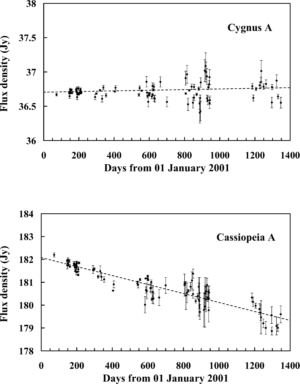
A convincing demonstration can be made of this calibration technique. The quality of the data corrected as described above can be assessed by intercomparing the 3 calibrators Jupiter, Cas A and Cyg A, all observed near transit and spread over the period 2002 to 2004. Fig. 2 shows plots of the observed flux density of Cyg A and Cas A using Jupiter as a calibrator. A similar plot for Tau A is given in Fig. 9 below. The daily scatter in the fluxes measured relative to Jupiter is seen to be % . The level of thermal noise in a typical daily measurement is Jy while the daily scatter is Jy, thus the variations are dominated by the atmosphere. In the case of Cyg A and Cas A, the time difference between the source and Jupiter observation can be as large as 12hr. For Tau A, where the time difference is smaller (hr) over this period, the scatter was %.
Since the main contributor to the scatter is atmospheric water vapour emission, the 1% scatter corresponds to 1% of set noise within the AGC system, which is 0.35 K. At 33 GHz this temperature scatter corresponds to 1 mm pwv (Danese & Partridge 1989). Some of the implications of this high level of stability in the atmosphere is included in the discussion of individual sources in sections 4.1 to 4.3.
4 Derived source parameters
We now derive the flux density and/or brightness temperature of our calibration sources at 33.0 GHz relative to Jupiter.
Since our results are most useful to the community working in the GHz wide band around 33 GHz, we have derived a spectral index for that range from flux densities in the literature (plus our new determinations). The brightness temperature spectrum of Jupiter has already been discussed in Section 3.3. We extrapolated all the VSA data to a common frequency of 33 GHz using the spectral indices derived from the literature.
For several of the sources in our study, data are available for time spans between 1 and 4 years. These accurate data are used to investigate source variability at high precision.
4.1 Cygnus A
Cyg A is a radio source associated with a double galaxy at a redshift of containing a central core and hot spots at the outer ends of diffuse radio lobes. The overall extent is 2.1 arcmin and is effectively unresolved in the compact and extended VSA arrays. No variability has ever been reported for Cyg A at any wavelength.
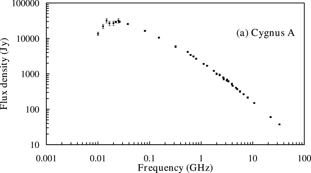
The radio spectrum of the integrated emission of Cyg A taken from literature is shown in Fig. 3. There are several changes of slope in the spectrum over the frequency range 0.1 to 100 GHz; one is at GHz and another is at GHz. The slope of the section 5-100 GHz, which includes 33 GHz, is . We recommend this as the spectral index at 33 GHz. This value may be compared with given in Table 3 of Baars et al. (1977) at similar frequencies.
| Frequency | S1965 | S2000 | Secular decrease |
|---|---|---|---|
| GHz | Jy | Jy | per year |
| 1.405 | 243950 | 197050 | 0.67 |
| 1.415 | 247050 | 188540 | 0.67 |
| 1.44 | 232850 | 179340 | 0.66 |
| 1.44 | 236720 | 181355 | 0.66 |
| 3.15 | 125838 | 103030 | 0.62 |
| 3.2 | 127958 | 100845 | 0.61 |
| 4.08 | 108426 | 86020 | 0.59 |
| 6.66 | 68420 | 54816 | 0.57 |
| 8.25 | 61522 | 49718 | 0.55 |
| 10.7 | 4680 | 3880 | 0.54 |
| 13.49 | 39413 | 32311 | 0.53 |
| 14.5 | 36710 | 3109 | 0.52 |
| 15.5 | 37618 | 30915 | 0.51 |
| 16 | 35411 | 2929 | 0.51 |
| 22.28 | 28510 | 2369 | 0.49 |
| 32 | 2246 | 1925 | 0.47 |
| 33 | 2115 | 1835 | 0.47 |
| 86 | 1154 | 1004 | 0.41 |
| 87 | 109.40 | 95.40 | 0.41 |
| 140 | 78.37 | 69.16.2 | 0.38 |
| 250 | 51.85.6 | 47.25.3 | 0.36 |
Observations of the calibration sources Cyg A, Cas A, and Jupiter were analysed for the period March 14 2001 to 4 May 2004. The flux density of Cyg A calibrated by Jupiter (assumed to have a brightness temperature of 146.6 K at 33 GHz) over this period is shown in Fig 2. In this period the RA of Jupiter ranged from RA=08h to 12h so observations were typically separated by 8-12 hr. The 1% scatter in the derived flux density of Cyg A was due to the atmosphere (mainly water vapour) over this time range. The mean flux density at 33 GHz was found to be 36.40.2 Jy.
These data can also be used to probe the long-term stability of the radio emission from Cyg A and Jupiter at 33 GHz. A fit to the data shows that the flux density ratio of Cyg A and Jupiter increases by 0.0430.039% per year. Accordingly we conclude that the relative radio emission changed by 0.1% per year over the period March 2001 to May 2004.
4.2 Cassiopeia A
Cas A is a 330-year old shell-type SNR of arcmin diameter. Baars et al. (1977) give its spectral index between 0.3 and 31 GHz as in 1965 and in 1980. Radio imaging shows multiple hot spots with spectral indices between and (see e.g. Anderson & Rudnick 1996) embedded in extended structure. Steeper spectra are associated with features thought to be bowshocks and with features outside the main radio ring; flatter spectra are found in the ring and in bright features within it which may account for its slow but measurable decrease in flux density with time at a rate which is thought to vary with frequency. These are important considerations when using Cas A as a calibrator.
4.2.1 The Cas A spectrum
Fig. 4 shows the spectrum of Cas A taken from published data over the frequency range 1.0 to 100 GHz with the flux densities corrected to the years 1965 and 2000 using the recipe given in Section 4.2.3 and listed in Table 2. The spectrum over this large frequency range shows a flattening of the spectral index above 15 GHz not detected in earlier data; this flattening is seen in both the 1965 and 2000 data. In 1965 at GHz and at GHz. For the 2000 data at GHz and at GHz. An appropriate spectral index at 33 GHz at the present epoch would appear to be .

4.2.2 VSA measurements of Cas A
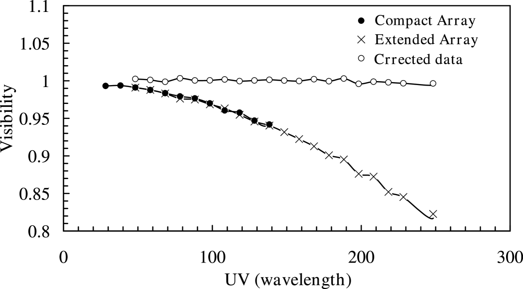
With the resolution of 17 and 11 arcmin for the compact and extended forms of the VSA, Cas A will show significant resolution effects in a project which aims for an accuracy of better than 1%. Accordingly, a correction was applied in the analysis procedure which scaled the visibilities on each baseline. The 5 GHz map from the VLA was used for this purpose. In view of the differing spectral indices within Cas A, it was necessary to confirm that the 5 GHz model was applicable to our 33 GHz observations. Fig. 5 which plots the visibility amplitude of Cas A versus the baseline length shows the results of this investigation. It can be seen that the normalised visibility after correction with the model is unity within 1% across the baseline range 20 to 250 . The compact and extended VSA data sets overlap at a precision of better than 0.5% in the baseline range 50-130 . The correction model is thus adequate for our purpose. Fig. 2(b) shows the flux density of Cas A measured over the period 13 March 2001 to 9 August 2004. Each point is the average of the flux densities measured relative to Cyg A and Jupiter. The secular decrease in the flux density of Cas A is clearly seen. No seasonal effects are evident in the data as the 3 sources move from day to night. Moreover the data for the compact array (March 2000 to May 2001) are entirely consistent with those from the extended array; no step is seen in the plot around May 2001. A linear fit to the data of Fig. 2(b) gives a flux density for Cas A on the adopted Jupiter scale of 182.020.07 Jy on January 2001. The linear rate of decrease over the period March 2001 to August 2004 is given by
| (6) |
4.2.3 Secular decrease in flux density of Cas A
The current estimate of the secular decrease in the flux density of Cas A at 33 GHz obtained over a 3.5 year period in the present decade is the most accurate of any epoch. Scott et al. (1969) at 81.5 MHz covering the two decades found a value of % yr-1. Using more recent data at 81.5 MHz, Hook et al. (1992) found a lower value rate of decrease between 1949 and 1989.7 of % yr-1.
We now re-examine the data available relating to the variability of Cas A as a function of both epoch and frequency. The data between 1949 and 1976 in the frequency range 81.5 MHz to 9.4 GHz indicated a secular decrease of flux density estimated by Baars et al. (1977) to be frequency dependent and given by the relation
| (7) |
The most accurate data currently available covers the frequency range 38 MHz to 33 GHz and the period 1949 to 2004 is given in Table 3.
| Frequency | Epoch | Decrease |
|---|---|---|
| GHz | % per year | |
| 0.038 | 1955-87 | 0.80.08 |
| 0.0815 | 1949-69 | 1.290.08 |
| 0.0815 | 1949-1989 | 0.920.16 |
| 0.0815 | 1965-1989 | 0.630.06 |
| 0.1025 | 1977-1992 | 0.800.12 |
| 0.927 | 1977-1996 | 0.730.05 |
| 0.950 | 1964-1972 | 0.850.05 |
| 1.405 | 1965-1999 | 0.620.12 |
| 1.420 | 1957-1976 | 0.890.02 |
| 1.420 | 1957-1971 | 0.890.12 |
| 3.000 | 1961-1972 | 0.920.15 |
| 3.060 | 1961-1971 | 1.040.21 |
| 7.800 | 1963-1974 | 0.70.1 |
| 9.400 | 1961-1971 | 0.630.12 |
| 15.500 | 1965-1995 | 0.60.06 |
| 33.000 | 2001-2004 | 0.390.02 |
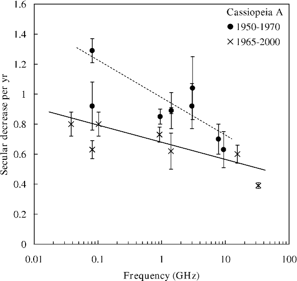
Fig. 6 shows the data from Table 3 divided into two epochs. The filled circles show the secular decrease from to 1970 while the crosses show the decrease from to 1990/2000. It is clearly evident that the earlier data shows higher ( 50%) secular decrease than the later data. The data from 1970 to 1990/2000 indicate a secular decrease of
| (8) |
The material available is not sufficient to show whether the fall in the secular rate is linear with time or is or not (as proposed for the 81.5 MHz data by Hook et al. (1992)). Apart from the current (2001-2004) 33 GHz result the values given by equation 6 may be an upper limit to the secular variation of Cas A at the present epoch. The secular decrease of Cas A will be discussed further in a related paper (Lancaster et al., in prep.).
A frequency-dependent secular variation has implications at the present epoch for the spectrum of Cas A. We can apply equation (7) to the higher weight data from Table 2 of Baars et al. (1977) and more recent data particularly at higher frequencies (Reichart & Stephens 2000, Mezger et al. 1986, Mason et al. 1999, Liszt & Lucas 1999, Wright et al. 1999, present paper) to derive spectra for 1965 (the Baars et al., epoch) and for 2000 at frequencies from 1 GHz to 250 GHz). The decrease of the secular term with frequency as shown by equation (7) gives a flattening of the spectral index with time. A synchrotron spectral index which flattens with time implies that particle acceleration is continuing in Cas A, presumably at the shock interfaces in the object (see e.g. Reynolds & Ellison 1992).
4.3 Taurus A
The Crab Nebula is the filled-centre remnant of the supernova of 1054 AD. The central neutron star remains active and replenishes the supply of relativistic electrons in the nebula. There is some evidence for a small secular decrease of the flux density at both radio and optical wavelengths. The present observations lead to a flux density of Tau A at 33 GHz. Since the source is strongly linearly polarized we must determine the polarization in order to use Tau A as a calibrator at 1% accuracy.
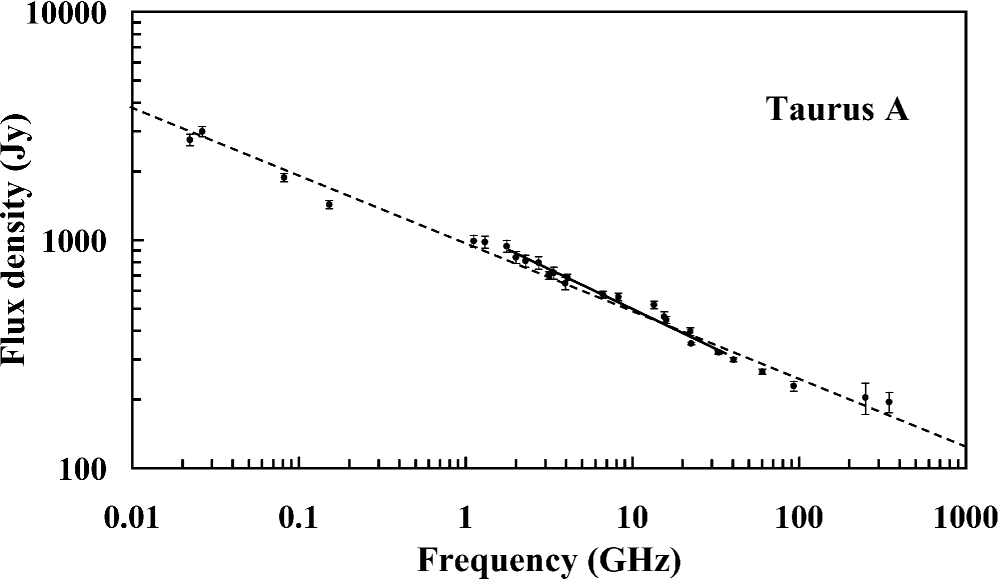
4.3.1 The spectrum of Tau A
Baars et al. (1977) found a constant spectral index over the frequency range 1-35 GHz with value of . More recent data, including higher frequencies up to 350 GHz are shown in Fig. 7. A constant spectral index of fits the data between 1 and 350 GHz. The expected turn-down of the spectrum is beyond this frequency range and is believed to be at 10 THz (Marsden et al. 1984). There is, however, some evidence for a small curvature of the spectrum. We find = between 22 and 1800 MHz, between 1.8 and 33 GHz and between 8 and 347 GHz. Green (2002) gives the spectral index between 1.5 and 347 GHz of individual structures in the nebula to lie in the range and . Similarly Mezger et al. (1986) give a spectral index between images at 10.7 and 250 GHz of . We adopt as an appropriate spectral index at GHz, which is consistent with the recent analysis by Macias-Perez et al. (2008).
4.3.2 The VSA observations of Tau A
Care is required when using Tau A as a calibrator in two regards. Firstly, it is an extended source with dimensions of 4 x 6 arcmin2 at position angle (pa) and consequently requires a resolution correction when observed with the VSA in both the extended and compact configurations. Secondly, it is some linearly polarized at frequencies of 30 GHz and above and this must be taken into account when observing with linear polarization.
The observed optical polarization of Tau A is at pa=159.6∘ (Oort and Walraven 1956). The integrated radio polarisation increases from 2% at 1.4 GHz to 7% at 5 GHz (Gardner & Davies 1966). The mean Faraday rotation measure (RM) in Tau A is rad m-2 with values up to 300 rad m-2 in some places. Any RM in this range leads to negligible Faraday rotation (FR) 30 GHz (a wavelength of 1.0 cm) corresponding to a FR 1∘ (FR).
We now consider the VSA data for Tau A.
-
1.
The linear polarization of Tau A. This can be estimated from long HA tracks of the source, remembering that the VSA is linearly polarized at pa=0∘. The maximum HA track for Tau A runs from HA=h 00m to h 00m. The observed data from the extended array on 26 December 2001 calibrated against Cas A (and Jupiter) is shown in Fig. 8 by crosses. This data set is first corrected (circles) for resolution effects of the VSA as for Cas A (section 4.2.2) using a 5 GHz map of Tau; this model was confirmed by showing that the corrected visibilities were constant with baseline for both the compact and extended VSA configurations in the manner illustrated for Cas A in Fig. 5. The elevation correction for absorption in the atmosphere and the AGC effect on the receivers (0.26 cosec - see Section 3.4) were then applied giving the true variation of flux density with HA shown as filled circles in Fig. 8. The linearly polarized flux density P is then estimated by fitting the corrected data to P cosec (2()), where is the polarization pa measured east from north and is the parallactic angle at the HA of observation. Data from 4 nights (26 December 2001, 09 February 2002, 12 October 2002 and 25 January 2003) of good weather and analysed as above were averaged to determine the polarization of Tau A. The results of this fitting gave P = 24.61.6 Jy corresponding to 7.80.6% linear polarisation at pa=148∘3∘. The errors quoted include the uncertainty in the atmospheric correction.
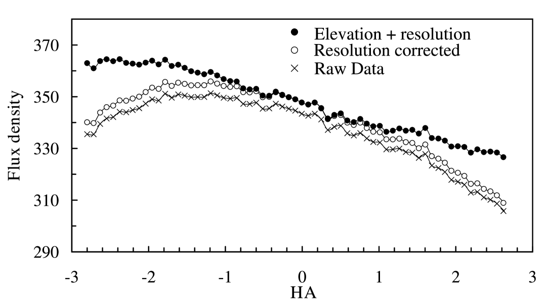
Figure 8: The flux density of Tau A plotted against HA for the observation on 26 December 2001 with the extended array. Crosses show the observed data calibrated against Jupiter; open circles show the data then corrected for resolution affects; filled circles show the data further corrected for elevation (atmospheric absorption and the AGC effect). The resultant sloping HA plot is due to the linear polarization of Tau A. -
2.
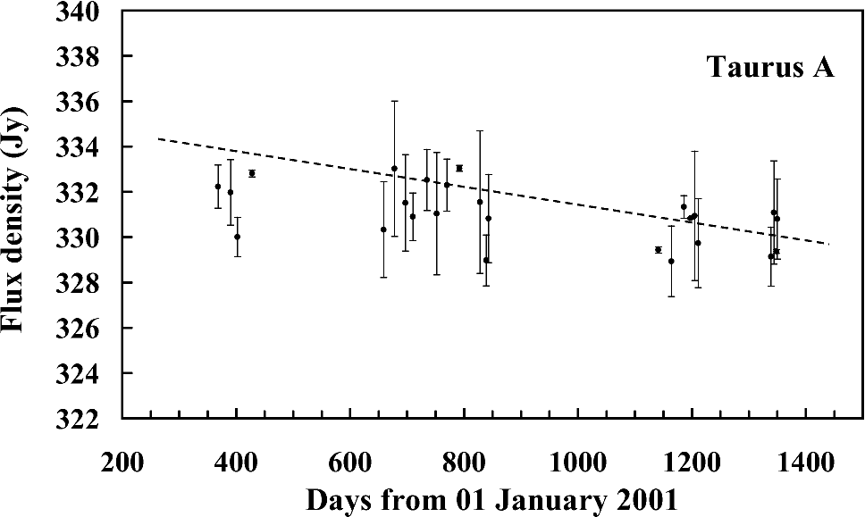
The flux density of Tau A at 33 GHz. The total flux density of Tau A is determined by the fitting procedure given in the previous section. The average of the 4 HA scans gives S(Tau A) = 322 4 Jy. The flux density of Tau A at HA = 0hr (pa = 0∘) is 332 4 Jy. A more extensive data set using short calibration tracks running from 3 January 2002 to 11 September 2004 with the extended array gave a more accurate estimate. The individual data points were corrected for resolution and for the atmosphere and are plotted in Fig. 9. The use of Jupiter as the reference for Tau A led to the very low scatter (rms = 0.4%) in the data since they were both night-time objects and separated in time by less than 5 hrs. This data set gives a flux density for Tau A at pa = 0∘ of 332.8 0.7 Jy on 1 January 2001. The secular decrease of Tau A indicated by Fig. 9 is discussed in the next section.
4.3.3 Secular decay of Tau A
The 950-year old nebula is clearly in the decay phase although centrally reenergised from the spindown of its central pulsar. Theoretical models predict a secular decrease of 0.16 to 0.4% per year at radio wavelengths (Reynolds and Chevalier 1984). An extended series of observations at 8.0 GHz over the period 1969-1985 by Aller & Reynolds (1985) gave a decrease of 0.1670.015% per year, a value consistent with the theoretical models (an interesting determination of the optical decay of the continuum at 5000 Angstrom using data from 1960 to 2002.2 has been made by Smith (2003) who found a decay of 0.50.2% per year).
The current 33 GHz observations of Tau A presented in Fig. 9 and described in the previous section give a secular decrease over the period January 2002 to September 2004 of
| (9) |
This is very similar to the value obtained by Aller & Reynolds (1985) at 8.0 GHz for the longer but earlier period 1968 to 1985 and is also consistent with the models of Reynolds & Chevalier (1984). A secular decrease of % per year would seem to be appropriate for the present epoch at 33 GHz.
4.4 NGC7027
NGC7027 is young planetary nebula which is optically thick in Lyman continuum and is therefore an ionization-bounded ionized hydrogen region. The radio continuum and optical nebula have dimensions of 12 x 8 arcsec2 (Basart & Daub 1987). It is surrounded by a ring of neutral molecular gas and dust some 40 arcsec in diameter possibly extending to 70 arcsec (see e.g. Hoare et al. 1992; Bieging et al. 1991). The expansion age of NGC7027 is 1200 yr with an expansion rate of 4.20.6 mas per year (Masson 1989).
Three factors are of particular interest in the present study. The first is the activity within the nebula; its expansion velocity is 17.51.5 kms-1 with local gas velocities up to 55 kms-1 (Lopez et al. 1998, Cox et al. 2002). These motions may lead to secular variations of radio flux density. The second effect is the clumpiness of the ionized gas in NGC7027 which results in optically thick knots up to at least 5 GHz (Bains et al. 2003). This determines the frequency range for which an optically thin radio thermal spectrum (at T14000 K) may be adopted. Thirdly, the dust within and surrounding NGC7027 may produce anomalous radio emission as in the case of the Helix Nebula (Casassus et al. 2004) and LDN 1622 (Casassus et al. 2006). Such emission, which peaks in the range 10-30 GHz (Draine & Lazarian 1998), needs to be considered when discussing the spectrum of NGC7027.
4.4.1 Spectrum of NGC7027
The radio spectrum of the integrated emission from NGC7027 is shown in Fig. 10 from the radio to the far infrared (FIR). It consists of several components. At radio frequencies the spectrum is due to free-free emission, optically thick at the lower frequencies and optically thin at the higher radio frequencies. The transition to optically thin occurs at 5-10 GHz in agreement with the observation by Bryce et al. (1997) that the bright NW knot has an optical depth of 2.0 at 5 GHz. A fit to the data between 10 and 80 GHz gives an optically thin spectral index of . The expected local value of the thermal spectral index for the observed electron temperature (14,000 K) in this frequency range lies between (at 10 GHz) and (43 GHz) (Dickinson et al. 2003).
The FIR emission consists of two components. One is warm (100 K) dust inside the arcsec2 ionized hydrogen region and the other is cool (30 K) dust in a neutral gas ring 40 arcsec in diameter surrounding the nebula (Hoare et al. 1992, Bieging et al. 1991). Both these dust components are covered by the observing beamwidth of the VSA and are included in the integrated emission described here.
The question of whether there is significant anomalous radio emission from either or both of the dust components can be addressed. There is no obvious emission with a peaked spectrum of roughly an octave width centred at GHz in the spectrum of Fig. 10. For a normal cool dust cloud the expected emission based on the 100 (3 THz) flux density would be Jy (Davies et al. 2006, Watson et al. 2005, Casassus et al. 2006). The emission from a normal HII region (Dickinson et al. 2006 & 2007) would be Jy. The latter is more consistent with Fig. 10.

4.4.2 The variability of NGC7027
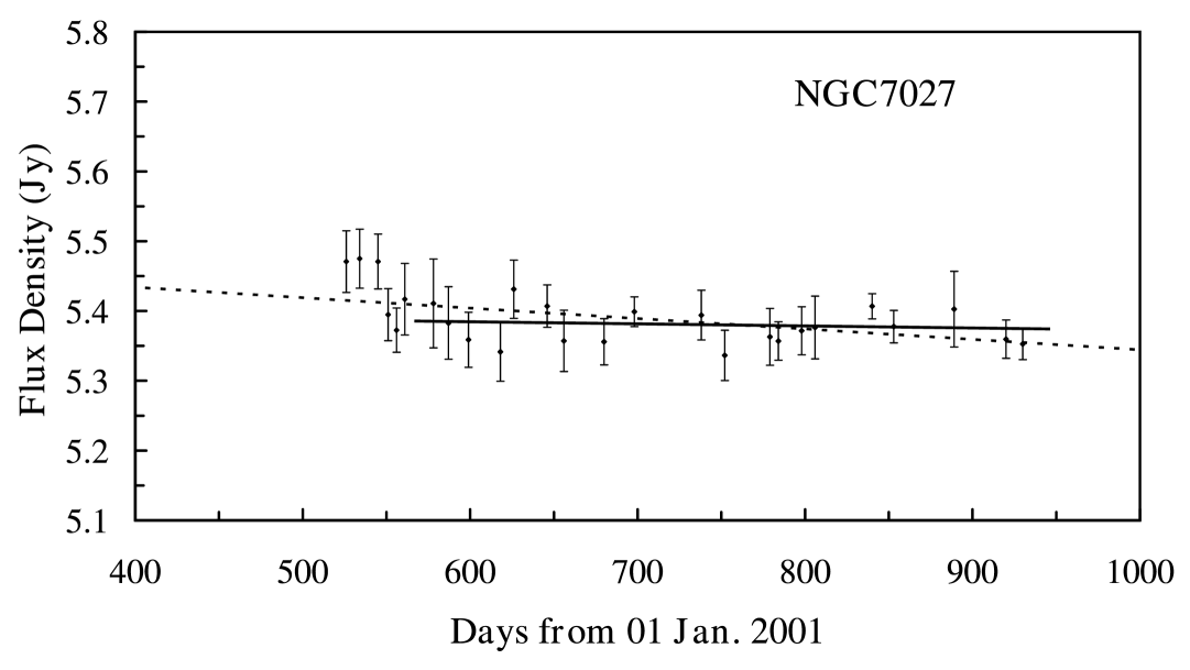
The flux densities measured over the period June 2002 to July 2003 are shown in Fig. 11. There is weak evidence for a higher flux density in the 6 observations before 10 July 2002. After this time the flux density remains constant for the year; a linear fit to the latter data gives an insignificant annual change of % yr-1. A fit to the full run of the data gives a decrease of 0.80.3% per year. The average flux density of NGC7027 in the period June 2002 to July 2003 is 5.390.04 Jy.
The long-term secular variation of NGC7027 at radio frequencies is often discussed (see e.g. Ott et al. 1994; Masson 1989). A substantial data set covering the frequency range 4.8 to 43 GHz is available in the literature extending back to 1967. Fig. 12 shows the flux density of NGC7027 from 1967 to 2003 in two frequency ranges: GHz where free-free self-absorption becomes significant and GHz where the spectrum is optically thin as can be seen in Fig. 10. All flux densities are corrected to a frequency of 33 GHz, assuming an optically thin spectral index as expected theoretically for this frequency range (Dickinson et al. 2003). The 4.8 - 6.6 GHz flux densities (median frequency 5.2 GHz) are 82 3% of the optically thin frequencies, indicating =0.18 at 5 GHz. Giving each point equal weight, the secular change in the flux density at optically thin frequencies (8.0 to 43 GHz) is
| (10) |
At the slightly optically thick frequencies (4.8 - 6.6 GHz)
| (11) |
when taking all the data. However, discarding the earlier data with larger errors, the secular change from 1975 to 1996 is
| (12) |
in close agreement with the optically thin data. We therefore have consistent results from two independent data sets. On combining the above data, we conclude that for NGC7027
| (13) |
over the period 1970 to the present.
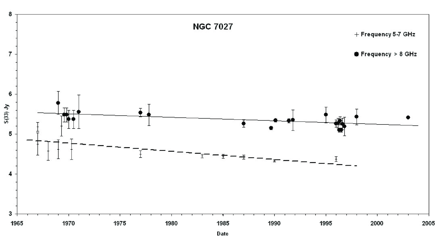
(a) Full line and filled circles; optically thin frequencies, 8.0 to 43 GHz, and
(b) dashed line and crosses; partially optically thick frequencies, 4.8 to 6.6 GHz.
After completion of this work Zijlstra, van Hoof & Perley (2008) published observations made with the VLA at frequencies in the range 1.275 to 43.34 GHz covering the period 1983-2006. They find that over this shorter period the flux density increases at lower frequencies where the emission is optically thick and decreases at higher (optically thin) frequencies. The turnover occurs between 2 and 4 GHz. Their value of decrease at optically thin frequencies of 0.145 0.005 % yr-1 is consistent to that of the present study covering data from the 36 year period to 2003.
4.5 Venus
The radio spectrum of Venus is the result of contributions from different depths in its atmosphere at high frequencies and from the surface at low frequencies. At the surface the temperature is K and the pressure bar. The millimetric emission arises from the higher atmosphere at h km where the effective temperature is 300 K. At intermediate radio frequencies the emission arises from the finite microwave opacity of SO2 and H2SO4. At 33 GHz where the brightness temperature is K the effective altitude of the emission is 35 km; this is the altitude at which space probes recorded a temperature of 460 K and a pressure of bar. At altitudes of 100 km a strong Venusian diurnal effect has been measured by space probes. We have examined our data to determine whether this diurnal effect extends down to altitudes around 35 km where the 33 GHz emission arises.
4.5.1 The spectrum of Venus
Fig. 13(a) shows the radio brightness temperature spectrum of Venus. The low frequencies come from the surface region where the temperature is 750 K. The higher GHz frequencies arise in successively higher levels in the Venusian atmosphere where temperatures are lower. The slope of the Tb spectrum at 33 GHz, estimated from a best fit to the range 10 to 100 GHz, is (the temperature spectral index, , is related to the flux density spectral index, , by ).
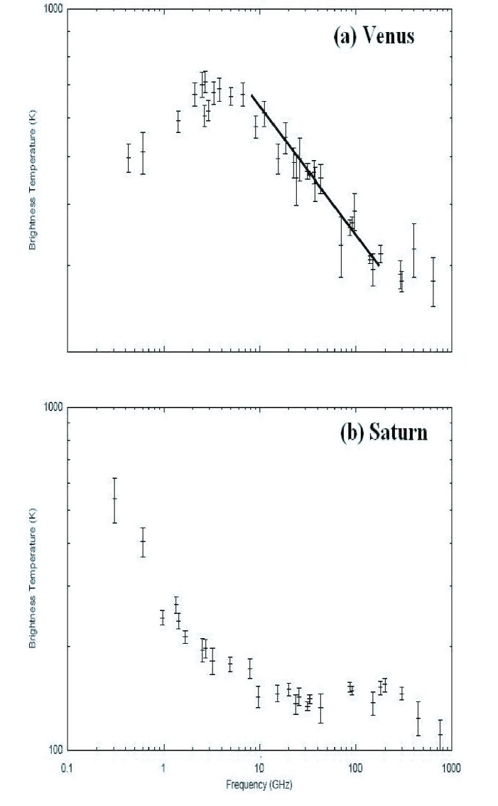
(b) The brightness temperature spectrum of Saturn from the literature.
4.5.2 Brightness temperature variation with illumination
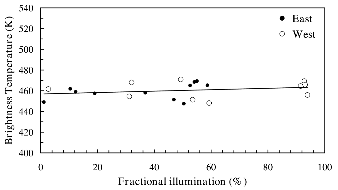
Fig. 14 shows the 33 GHz brightness temperature of Venus as a function of illumination for the period August 2002 to September 2004. During this period, Venus went through 1.5 Synodic cycles. Data are shown separately for eastern and western illumination, corresponding to times when the Venusian surface was entering or leaving the long period of darkness. No difference is seen between these two phases of illumination of more than 2 K ( 0.3 %). The variation of brightness temperature with illumination suggests a weak increase of temperature with illumination of +1.51.3% (6.96.0 K) from zero to full illumination.
4.6 Saturn
Saturn is used as a secondary calibrator by the VSA. For accurate measurements the effect of the rings must be taken into account. The rings themselves emit with a brightness temperature of 10-20 K and also block out the emission from the disk of Saturn (see for example Janssen & Olsen 1978, Conway 1980; Ulich 1981). As a consequence, the effective brightness temperature of Saturn varies with the tilt angle B (the Saturnicentric latitude of the earth). We present data for the period June 2002 to August 2003.
4.6.1 The spectrum of Saturn
The microwave spectrum of Saturn taken from the literature is plotted in Fig. 13(b) in terms of its brightness temperature. There is some uncertainty as to the contribution of the rings to the data presented. Since the ring effect is typically less than 5 percent, it lies within the error assigned to most data points in Fig 13(b). The shape of the spectrum is quantitatively similar to that of Jupiter - increasing from K at mm wavelengths to 540 K at 94 cm. As in the case of Jupiter there is evidence for the presence of ammonia as the principle source of opacity at radio frequencies with its inversion band at GHz. At 30 GHz the frequency of interest in the present study, the effective temperature spectral index is = 0.000.05. At frequencies of GHz, , while at GHz, .
4.6.2 Secular variation of Saturn at 33 GHz
The VSA programme gave an accurate data set for the integrated flux density of Saturn extending from 29 June 2002 to 02 August 2003. During this period the tilt angle moved between B = 26∘ and 27∘ with a quasi - annual period. The brightness temperature is then calculated by assuming the observed flux density arises from Saturn’s disk whose dimensions are given in the Ephemeris. Fig 15 is the brightness temperature plot over this period and shows no secular variation greater than 0.4% per year at 95% confidence level. Our results indicate that the mean brightness temperature of Saturn (disk plus rings) between June 2002 and August 2003 is 140.500.12 K; for the data set the mean tilt angle B = 26.5∘.

5 Conclusion
We have determined the flux density or brightness temperature at 33 GHz of 7 sources used by the VSA for calibration; the results are summarised in Tables 4 & 5. This list includes sources widely used for calibration in this frequency range in radio-source and CMB studies; they are the strong sources and planets. The high level of reliability of the VSA and the stable atmosphere at the Izaña site have assured accurate relative measurements of these sources. We use Jupiter as the reference standard in this work and adopt a brightness temperature of 146.60.75 K at 33 GHz as determined in the WMAP survey (Hill et al. 2008). Any refinement in the future can then be applied to the present results. In order to make our results useful for accurate flux density/brightness temperature measurements in the frequency band around 33 GHz we derive a spectral index from published data.
| Radio sources | dS/Sdt (% yr-1) |
|---|---|
| Cas A | |
| Tau A | |
| NGC70271 | |
| Cyg A | |
| Venus2 | |
| 1 At optically thin frequencies; see Section 4.4.2. | |
| 2 Secular variation of Tb with illumination; see Section 4.5.2. | |
Since we have observations of the calibrators extending over nearly 4 years, we are able to make an accurate assessment of the calibrator variation over this period. With rms individual comparison measurements of 0.4 to 1.0 % depending on the time separation of the pair of observations, we are sensitive to small secular flux density or brightness temperature variations. A significant secular decrease in flux density was established for Cas A and Tau A over the 4-year observing period. By combining our data with historical data in the literature, we have also demonstrated a significant secular decrease for NGC7027 at optically thin frequencies. Over this period the secular variation of the two sources expected not to vary, Cyg A and Jupiter, was less than 0.1% yr-1. Venus showed a slight (1.51.3%) variation with illumination.
| Radio sources | Flux density | Error | Spectral index |
| (Jy) | (Jy) | (at 33 GHz) | |
| Cas A | 182.0 | 0.1 | |
| Cyg A | 36.4 | 0.2 | |
| Tau A1,2 | 322 | 4 | |
| NGC70273 | 5.39 | 0.04 | |
| Planets | Brightness temperature | Error | Spectral index |
| (K) | (K) | (at 33 GHz) | |
| Jupiter | 146.6 | 0.75 | |
| Venus | 460.3 | 3.2 | |
| Saturn4 | 140.50 | 0.12 | |
| 1Tau A is 7.80.6% yr-1 linearly polarized at pa . | |||
| 2Tau A flux density is 332.80.7 Jy at pa = 0∘. | |||
| 3Flux density at 2003.0. | |||
| 4Flux density at 2003.0; tilt angle B of rings is 26.5∘. | |||
Acknowledgements
YH thanks the King Abdul City of Science and Technology for support. CD acknowledges support from the U.S. Planck project, which is funded by the NASA Science Mission Directorate.
References
- Aller & Reynolds (1985) Aller, H. D., & Reynolds, S. P. 1985, Proceedings of Workshop, The Crab Nebula and Related Supernova Remnants, 75
- Anderson & Rudnick (1996) Anderson, M. C., & Rudnick, L. 1996, ApJ, 456, 234
- Baars et al. (1977) Baars, J. W. M., Genzel, R., Pauliny-Toth, I. I. K., & Witzel, A. 1977, AAP, 61, 99
- Bains et al. (2003) Bains, I., Bryce, M., Mellema, G., Redman, M. P., & Thomasson, P. 2003, MNRAS, 340, 381
- Basart & Daub (1987) Basart, J. P., & Daub, C. T. 1987, ApJ, 317, 412
- Bieging et al. (1991) Bieging, J. H., Wilner, D., & Thronson, H. A., Jr. 1991, ApJ, 379, 271
- Bryce et al. (1997) Bryce, M., Pedlar, A., Muxlow, T., Thomasson, P., Mellema, G., 1997, MNRAS, 284, 815
- Casassus et al. (2004) Casassus, S., Readhead A. C. S., Pearson T. J., Nyman L.-A., Shepherd M. C., Bronfman L., 2004, ApJ, 603,599
- Casassus et al. (2006) Casassus, S., Cabrera, G. F., Forster, F., Pearson, T. J., Readhead, A. C. S., Dickinson, C., 2006, ApJ, 639, 951
- Conway (1980) Conway, R. 1980, MNRAS, 190, 169
- Cox et al. (2002) Cox, P., Huggins, P. J., Maillard, J.-P., Habart, E., Morisset, C., Bachiller, R., & Forveille, T. 2002, A&A, 384, 603
- Danese & Partridge (1989) Danese, L., & Partridge, R.B. 1989, ApJ, 342, 604
- Davies et al. (1996) Davies, R. D., et al. 1996, MNRAS, 278, 883
- Davies et al. (2006) Davies, R. D., Dickinson, C., Banday, A. J., Jaffe, T. R., Górski, K. M., & Davis, R. J. 2006, MNRAS, 370, 1125
- Dickinson et al. (2003) Dickinson, C., Davies, R. D., & Davis, R. J. 2003, MNRAS, 341, 369
- Dickinson et al. (2004) Dickinson, C., et al. 2004, MNRAS, 353, 732
- Dickinson et al. (2006) Dickinson, C., Casassus, S., Pineda, J.L., Pearson, T.J., Readhead, A.C.S., & Davies, R.D. 2006, ApJ, 643, L111
- Dickinson et al. (2007) Dickinson, C., et al. 2007, MNRAS, 379, 297
- Draine & Lazarian (1998) Draine, B. T., & Lazarian, A. 1998, ApJ, 508, 157
- Gardner & Davies (1966) Gardner, F. F., & Davies, R. D. 1966, Australian Journal of Physics, 19, 441
- Genova-Santos et al. (2008) Genova-Santos, R., et al., 2008, MNRAS, submitted (arXiv:0804.0199)
- Green. (2002) Green, D. A., 2002, Neutron Stars in Supernova Remnants, ASP conference series, 271, 153
- Gulkis et al. (1974) Gulkis, S., Klein, M. J., & Poynter, R. L. 1974, IAU Symposium 65, Exploration of the Planetary System, p367
- Hill et al. (2008) Hill, R.S. et al., 2008, ApJ, submitted (arXiv:0803.0570)
- Hinshaw et al. (2008) Hinshaw, G. et al., 2008, ApJ, submitted (arXiv:0803.0732)
- Hoare et al. (1992) Hoare, M. G., Roche, P. F., & Clegg, R. E. S. 1992, MNRAS, 258, 257
- Hook et al. (1992) Hook, I. M., Duffett-Smith, P. J., & Shakeshaft, J. R. 1992, A&A, 255, 285
- Janssen & Olsen (1978) Janssen, M. A., & Olsen, E. T. 1978, Icarus, 33, 263
- Liszt & Lucas (1999) Liszt, H., & Lucas, R. 1999, A&A, 347, 258
- Lopez et al. (1998) Lopez, J. A., Meaburn, J., Bryce M., Holloway, A. J. 1998, ApJ, 493, 803
- Macias-Perez et al. (2008) Macias-Perez, J. F., Mayet, F., Desert, F. X., Aumont, J., 2008, A&A, submitted (arXiv:0802.0412)
- Maisinger et al. (2003) Maisinger, K., Hobson, M. P., Saunders, R. D. E., & Grainge, K. J. B. 2003, MNRAS, 345, 800
- Marsden et al. (1984) Marsden, P. L., Gillett, F. C., Jennings, R. E., Emerson, J. P., de Jong, T., & Olnon, F. M. 1984, ApJL, 278, L29
- Mason et al. (1999) Mason, B. S., Leitch, E. M., Myers, S. T., Cartwright, J. K., & Readhead, A. C. S. 1999, AJ, 118, 2908
- Masson (1989) Masson, C. R. 1989, ApJ, 336, 294
- Mezger et al. (1986) Mezger, P. G., Tuffs, R. J., Chini, R., Kreysa, E., & Gemuend, H.-P. 1986, A&A, 167, 145
- Oort & Walraven (1956) Oort, J. H., & Walraven, T. 1956, BAIN, 12, 285
- Ott et al. (1994) Ott, M., Witzel, A., Quirrenbach, A., Krichbaum, T. P., Standke, K. J., Schalinski, C. J., & Hummel, C. A. 1994, A&A, 284, 331
- Page et al. (2003) Page, L., et al. 2003, ApJS, 148, 39
- Readhead et al. (2004) Readhead, A. C. S., et al. 2004, ApJ, 609,498
- Reichart & Stephens (2000) Reichart, D.E., & Stephens, A.W. 2000, ApJ, 537, 904
- Reynolds & Chevalier (1984) Reynolds, S. P., & Chevalier, R. A. 1984, ApJ, 278, 630
- Reynolds & Ellison (1992) Reynolds, S. P., & Ellison, D. C. 1992, American Institute of Physics Conference Series, 254, 455
- Scott et al. (1969) Scott, P. F., Shakeshaft, J. R., & Smith, M. A. 1969, Nat, 223, 1139
- Scott et al. (2003) Scott, P. F., et al. 2003, MNRAS, 341, 1076
- Smith (2003) Smith, N. 2003, MNRAS, 346, 885
- Taylor et al. (2003) Taylor, A.C., et al. 2003, MNRAS, 341, 1066
- Ulich (1981) Ulich, B. L. 1981, AJ, 86, 1619
- Watson et al. (2003) Watson, R. A., et al. 2003, MNRAS, 341, 1057
- Watson et al. (2005) Watson, R. A., Rebolo, R., Rubiño-Martín, J. A., Hildebrandt, S., Gutiérrez, C. M., Fernández-Cerezo, S., Hoyland, R. J., & Battistelli, E. S. 2005, ApJL, 624, L89
- Winter (1964) Winter, S. 1964, Tech. Note, Series 5, Issue 23, Space Sci Lab., UC Berkeley
- Wright et al. (1999) Wright, M., Dickel, J., Koralesky, B., & Rudnick, L. 1999, ApJ, 518, 284
- Zijlstra et al. (2008) Zijlstra, A. A., van Hoof, P.A.M., Perley, R.A., 2008, ApJ, submiited (arXiv:0801.3327)