Three-fluid plasmas in star formation
I. Magneto-hydrodynamic equations

Abstract

Context. Interstellar magnetic fields influence all stages of the process of star formation, from the collapse of molecular cloud cores to the formation and evolution of circumstellar disks and protostellar jets. This requires us to have a full understanding of the physical properties of magnetized plasmas of different degrees of ionization for a wide range of densities and temperatures.

Aims. We derive general equations governing the magneto-hydrodynamic evolution of a three-fluid medium of arbitrary ionization, also including the possibility of charged dust grains as the main charge carriers. In a companion paper (Pinto & Galli 2007), we complement this analysis computing accurate expressions of the collisional coupling coefficients for a variety of gas mixtures relevant for the process of star formation.

Methods. Over spatial and temporal scales larger than the so-called large-scale plasma limit and the collision-dominated plasma limit, and for non-relativistic fluid speeds, the electric field, the electric current and the ion-neutral drift have their instantaneous values determined by the evolution of the magnetic field, which obeys an advection-diffusion equation. The validity of the approximations made is discussed critically.

Results. We derive the general expressions for the resistivities, the diffusion time scales and the heating rates in a three-fluid medium and we use them to estimate the evolution of the magnetic field in molecular clouds and protostellar jets. Collisions between charged particles significantly increase the value of the Ohmic resistivity during the process of cloud collapse, affecting in particular the decoupling of matter and magnetic field and enhancing the rate of energy dissipation. The Hall resistivity can take larger values than previously found when the negative charge is mostly carried by dust grains. In weakly- or mildy-ionized protostellar jets, ambipolar diffusion is found to occur on a time scale comparable to the dynamical time scale, limiting the validity of steady-state and nondissipative models to study the jet’s structure.

1 Introduction

The interstellar medium (ISM) is a partially-ionized gas containing substantial fractions of neutral particles, mostly H and H₂, and several charged atomic and molecular species. About 2% of the mass of the ISM is in the form of solid particles (dust grains) with sizes ranging from $\sim 10$ Å to $\sim 1$ $\mu$m that may carry electric charge (Spitzer 1978, Nakano & Umebayashi 1980, 1986). The transformation of a piece of ISM into a protostar involves variations of several orders of magnitude in density, temperature, and ionization fraction, resulting in a variety of interconnected environments, such as cold dense clouds, cicumstellar disks, and protostellar jets. Magnetic fields affect the motion of the charged component of the gas, which in turn transfers the effects of the Lorentz force to the neutrals by elastic collisions.

While several authors have focused on specific ionization regimes or chemical compositions, we lack a rigorous formulation of the magneto-hydrodynamic (MHD) equations in general valid for the variety of situations occurring in the star formation process. First, the standard expressions of the plasma conductivities are generally derived neglecting the electron’s mass with respect to the ion and neutral’s masses (e.g., Braginski 1965, Mitchner & Kruger 1973), and are not applicable to conditions where the carriers of negative charge are dust grains rather than electrons. For example, charged dust grains dominate over free electrons in clouds cores of neutral density $\sim 10^{4}$–$10^{5}$ cm^-3 if a large number of very small grains is present (Nishi, Nakano & Umebayashi 1991), or during the collapse of molecular clouds when the neutral density becomes larger than $\sim 10^{7}$ cm^-3 (Nakano et al. 2002). Second, many of the commonly adopted expressions for the conductivity of the ISM in collapsing clouds and protostellar jets are derived neglecting collisions between charged particles (e.g., Wardle & Ng 1999; Desch & Mouschovias 2001; Nakano, Nishi & Umebayashi 2002; Tassis & Mouschovias 2005). This so-called “multifluid approach” can be used for an arbitrary number of charged species of arbitrary mass, but is valid only for low-ionization degrees and cannot be generalized to include collisions between charged particles in a self-consistent way (see e.g., Kelley 1989). Benilov (1996, 1997) derived the multifluid equations for a nonmagnetized plasma in detail, including accurate expressions for the rate of momentum transfer by elastic and inelastic collisions.

Following a different approach, in this paper we derive the general equation for the evolution of the magnetic field in a gas of arbitrary ionization degree made of positively- and negatively-charged particles and neutrals. We also obtain the general expressions of the resistivity coefficients, the associated timescales, and the heat generation rates for a three-fluid plasma. In a companion paper (Pinto & Galli 2007, hereafter Paper II), we compute accurate numerical and analytical expressions for the collisional coupling coefficients that are required to calculate the resistivity coefficients of the plasma. As an illustration, we apply the formalism derived in this paper to study the evolution of the magnetic field in a molecular cloud and in a protostellar jet with the help of simple analytical models. The same formalism can be adopted to study other situations such as e.g., multicomponent radiatively-driven stellar winds (Krtička & Kubát 2001) and shock waves in plasmas of low-ionization degree (Mullan 1971, Draine 1980, Draine & McKee 1993; Guillet, Pineau des Forêts & Jones 2007).

In Sect. 2 we develop a rigorous three-fluid theory for plasmas of arbitrary degree of ionization and particle masses, critically discussing the approximations made in deriving the governing equations; in Sect. 3 we obtain the complete advection-diffusion equation for the magnetic flux for an axially-symmetric system; in Sect. 4 we obtain the equation for the rate of energy generation due to friction forces between the fluid components; in Sect. 5 and in Sect. 6 we apply the three-fluid equations to typical conditions of molecular clouds and protostellar jets, respectively, evaluating the relevant evolutionary timescales and the heating rates; finally, in Sect. 7, we summarize our conclusions.

2 Three-fluid description of a partially-ionized gas

We consider a system composed by three fluids, namely positively-charged particles (subscript $+$), negatively-charged particles ($-$), and neutrals ($n$). The generic species $s$ (with $s=+,-,n$) is characterized by particle mass $m_{s}$, density $\rho_{s}$, mean flow velocity ${\bf u}_{s}$ and charge $q_{s}$, with $q_{-}=-Z_{-}e$ and $q_{+}=Z_{+}e$, where $e$ is the electron charge. Charged particles may include electrons ($e$), ions ($i$) and positively- or negatively-charged dust grains ($g^{+}$,$g^{-}$). We define the quantity

$$\epsilon\equiv\frac{Z_{+}m_{-}}{Z_{-}m_{+}},$$ (1)

the mass ratio of negatively- and positively-charged species. No assumption is made on the magnitude of $\epsilon$: for a plasma of ions and electrons, $\epsilon\ll 1$; for a plasma of ions and negatively-charged grains, $\epsilon\gg 1$; for a plasma of negatively- and positively-charged grains, $\epsilon\approx 1$.

In the following, and in Paper II, we specialize to the case where the fluid components are characterized by a maxwellian velocity distribution function with temperatures $T_{s}$, that is not necessarily the same for all species. Necessary conditions for this assumption are that (i) the characteristic evolution timescale of the system must be much longer than the inverse of the collision frequency between particles of a given species and (ii) the drift velocity between particles of different species must be sufficiently small to produce a frictional heating rate smaller than the thermal energy density of each component divided by its self-relaxation time (Draine 1986). The assumption of a maxwellian velocity distribution is equivalent to assume that the stress tensor is diagonal and, therefore, to neglect viscosity and heat conduction in the fluid (see Sect. 2.1).

The plasma is also electrically neutral,

$$\sum_{s}\frac{q_{s}}{m_{s}}\rho_{s}=0,$$ (2)

or, by Eq. (1),

$$\rho_{-}=\epsilon\rho_{+}.$$ (3)

The assumption of charge neutrality is valid if the characteristic length scale of the system is much larger than the Debye length of the charged particles (see Sect. 2.8 and Paper II).

2.1 Definitions

The mean velocity of each species averaged over its maxwellian velocity distribution function $f_{s}({\bf v}_{s})$ is given by

$${\bf u}_{s}\equiv\langle{\bf v}\rangle_{s}=\frac{\int{\bf v}_{s}f_{s}({\bf v}_{s})\;d{\bf v}_{s}}{\int f_{s}({\bf v}_{s})\;d{\bf v}_{s}},$$ (4)

where ${\bf v}_{s}$ is the microscopic velocity of the particles, and $f_{s}({\bf v})$ is normalized as

$$\int f_{s}({\bf v})\;d{\bf v}=1.$$ (5)

We also define the mass fractions of the three fluids,

$$\xi_{s}\equiv\frac{\rho_{s}}{\rho},$$ (6)

with $\sum_{s}\xi_{s}=1$. The average density and velocity of the three-fluid system are

$$\rho\equiv\sum_{s}\rho_{s},$$ (7)

and

$${\bf U}\equiv{1\over\rho}{\sum_{s}\rho_{s}{\bf u}_{s}},$$ (8)

respectively.

It is convenient to identify the random component of the microscopic velocity of each species with respect to the average fluid velocity ${\bf U}$. Therefore, we define

$${\bf v}_{s}={\bf U}+{\bf w}_{s},$$ (9)

so that

$${\bf u}_{s}=\langle{\bf U+w}\rangle_{s}={\bf U}+\langle{\bf w}\rangle_{s},$$ (10)

where $\langle\;\rangle_{s}$ indicates the average performed on the distribution function of the particles of species $s$.

Consistent with the assumption of a maxwellian velocity distribution, the pressure tensor for each species $P_{s}^{jk}=\rho_{s}\langle w_{j}w_{k}\rangle_{s}$ is diagonal,

$$P_{s}^{jk}=P_{s}\delta_{jk},\leavevmode\nobreak\ \leavevmode\nobreak\ \leavevmode\nobreak\ \mbox{with}\leavevmode\nobreak\ \leavevmode\nobreak\ \leavevmode\nobreak\ P_{s}=\frac{1}{3}\rho_{s}\langle w^{2}\rangle_{s}.$$ (11)

It is possible then to define the kinetic temperature $T_{s}$

$${3\over 2}k_{B}T_{s}\equiv{1\over 2}m_{s}\langle w^{2}\rangle_{s},$$ (12)

where $k_{B}$ is the Boltzmann’s constant, and the thermal speed $a_{s}$ for each species

$$a_{s}^{2}\equiv\frac{k_{B}T_{s}}{m_{s}},$$ (13)

in terms of the mean random energy of each component. Notice that this definition of temperature is based on the microscopic velocities of each species with respect to the average fluid, not with respect to the mean velocity of each species.

With these definitions, the pressure of each component is then given by

$$P_{s}=a_{s}^{2}\rho_{s}.$$ (14)

Since the random components ${\bf w}_{s}$ of the velocity of the different species are defined with respect to the same frame of reference (the one in which the center of mass is at rest), the pressure contributions of each species can be consistently added together to form the total pressure of the average fluid,

$$P\equiv\sum_{s}P_{s}=a^{2}\rho,\leavevmode\nobreak\ \leavevmode\nobreak\ \leavevmode\nobreak\ \mbox{where}\leavevmode\nobreak\ \leavevmode\nobreak\ \leavevmode\nobreak\ a^{2}\equiv\sum_{s}\xi_{s}a_{s}^{2}.$$ (15)

We also define the total density and pressure of the charged species as

$$\rho_{c}\equiv\rho_{+}+\rho_{-},\qquad P_{c}\equiv P_{+}+P_{-}.$$ (16)

We stress that this formulation, commonly adopted in plasma physics, (see, e.g., Krall & Trivelpiece 1973, Boyd & Sanderson 1969), is different from the approach adopted in the astrophysical literature (e.g., Mouschovias 1991)where the random velocity of each species is defined as a deviation with respect to the mean velocity of the same species, ${\bf v}_{s}={\bf u}_{s}+{\bf w}_{s}^{\prime}$. With the latter definition, the derivation of the fluid equations for each species is simplified by the fact that the average of the random components $\langle{\bf w^{\prime}}\rangle_{s}$ are zero. However, the pressure and the heat tensor defined in this way have a different meaning with respect to the corresponding quantities in our derivation. Although the partial pressures defined in the two approaches are nearly equivalent when ${\bf u}_{s}\approx{\bf U}$, the definitions adopted in the two cases, however, differ from a conceptual point of view, because in our approach the random components of the velocity of each species are defined in the same reference frame, and the partial pressures can be added to form physically meaningful global quantities.

By eq. (3), the electric current is

$${\bf J}\equiv\sum_{s}\frac{q_{s}}{m_{s}}\rho_{s}{\bf u}_{s}=-\frac{q_{-}}{m_{-}}\rho_{-}({\bf u}_{+}-{\bf u}_{-}).$$ (17)

Following Schlüter (1950, 1951), we also define an “ambipolar current” ${\bf J}_{d}$ associated to the ion-neutral drift speed ${\bf u}_{+}-{\bf u}_{n}$,

$${\bf J}_{d}\equiv-{q_{-}\over m_{-}}\rho_{c}({\bf u}_{+}-{\bf u}_{n}).$$ (18)

2.2 Equations of continuity and momentum

Taking the zeroth and first order momenta of the Boltzmann equation for each species, the equations of continuity and momentum read:

$$\frac{\partial\rho_{s}}{\partial t}+\nabla\cdot(\rho_{s}{\bf u}_{s})=\sum_{s^{\prime}}S_{ss^{\prime}},$$ (19)

$$\frac{\partial}{\partial t}(\rho_{s}{\bf u}_{s})+\nabla\cdot(\rho_{s}\langle{\bf v}{\bf v}\rangle_{s})=-\rho_{s}\nabla{\cal V}$$ (20)

$$+\frac{q_{s}\rho_{s}}{m_{s}}\left({\bf E}+\frac{{\bf u}_{s}}{c}\times{\bf B}\right)+\sum_{s^{\prime}}{\bf F}_{ss^{\prime}}+\sum_{s^{\prime}}{\bf r}_{ss^{\prime}},$$

where ${\cal V}$ is the gravitational potential, ${\bf E}$ is the electric field, ${\bf B}$ is the magnetic field, ${\bf F}_{ss^{\prime}}$ is the friction force (per unit volume) exerted on particles of the fluid $s$ by particles of the fluid $s^{\prime}$ by elastic collisions, $S_{ss^{\prime}}$ and ${\bf r}_{ss^{\prime}}$ are the rate of change of density and momentum of the species $s$ due to inelastic collisions (chemical reactions) with particles of species $s^{\prime}$.

2.3 Elastic collisions

The calculation of the friction force ${\bf F}_{ss^{\prime}}$ accounting for elastic collisions between particles with a Maxwellian velocity distribution is reviewed in Paper II. The resulting expression is

$${\bf F}_{ss^{\prime}}=\alpha_{ss^{\prime}}({\bf u}_{s^{\prime}}-{\bf u}_{s}),$$ (21)

where $\alpha_{ss^{\prime}}$ is the so-called friction coefficient, related to the momentum transfer rate coefficient $\langle\sigma v\rangle_{ss^{\prime}}$ by

$$\alpha_{ss^{\prime}}\equiv\frac{\rho_{s}\rho_{s^{\prime}}}{m_{s}+m_{s^{\prime}}}\langle\sigma v\rangle_{ss^{\prime}}.$$ (22)

For elastic collisions, $\alpha_{ss^{\prime}}=\alpha_{s^{\prime}s}$, and therefore ${\bf F}_{ss^{\prime}}=-{\bf F}_{s^{\prime}s}$. In general, $\langle\sigma v\rangle_{ss^{\prime}}$ is a function of the temperatures $T_{s}$ and $T_{s^{\prime}}$ and of the relative mean velocity $|{\bf u}_{s^{\prime}}-{\bf u}_{s}|$ of the interacting species. Thus, ${\bf F}_{ss^{\prime}}$ is a nonlinear function of the relative mean velocity. Accurate values of $\langle\sigma v\rangle_{ss^{\prime}}$ for various colliding particles, and useful fitting formulae for a wide range of temperatures and drift velocities, are derived in Paper II.

Another frequently used quantity is the collisional drag coefficient

$$\gamma_{ss^{\prime}}\equiv\frac{\langle\sigma v\rangle_{ss^{\prime}}}{m_{s}+m_{s^{\prime}}},$$ (23)

which is independent on the particle’s density.

2.4 Inelastic collisions

The expressions for the rate of change of momentum due to inelastic collisions depend on the specific type of chemical reaction considered. For binary reactive collisions that produce one or two particles, Benilov (1996) has found that

$${\bf r}_{ss^{\prime}}=\alpha_{ss^{\prime}}^{\rm inel.}({\bf u}_{s^{\prime}}-{\bf u}_{s})+S_{ss^{\prime}}{\bf u}_{s},$$ (24)

where $\alpha^{\rm inel.}_{ss^{\prime}}$ is a complex function of the masses and temperatures of the two reacting species, their relative mean velocity, and the reaction cross section (or the reaction rate). Approximated expressions for $\alpha_{ss^{\prime}}^{\rm inel.}$ have been obtained by Draine (1986) for several specific reactions, and by Ciolek & Mouschovias (1993) for reactions involving dust grains.

Within a three-fluid scheme like the one considered in this paper, the only possible reactions between two species of particles are recombinations of singly-charged ions with electrons, resulting in the production of neutral particles ($i+e\rightarrow n$) and ionization reactions ($n\rightarrow i+e$) . A multifluid scheme is more appropriate when explicitly considering chemical reactions and the associated change of mass and momentum, as, for example, in the dynamics of shock waves in the ISM (Flower, Pineau des Fôrets & Hartquist 1985, Draine 1986) or the collapse of magnetized molecular clouds (Ciolek & Mouschovias 1993).

In the following, we make the hypothesis that gas is not subject to ionization, recombination, or other chemical reactions that contribute to the transfer of momentum from one fluid to the other. In other words, we restrict ourselves to the study of nonreacting MHD flows.

2.5 Equations for the mean fluid

Neglecting the rate of change of density and momentum of each species by chemical reactions ($S_{ss^{\prime}}={\bf r}_{ss^{\prime}}=0$), the equations of continuity and momentum for the mean fluid can be easily derived summing the equations (19) and (20) over the species $s$,

$$\frac{D\rho}{Dt}+\rho\nabla\cdot{\bf U}=0,$$ (25)

$$\rho\frac{D{\bf U}}{Dt}=-\nabla P-\rho\nabla{\cal V}+\frac{\bf J}{c}\times{\bf B},$$ (26)

where $D/Dt=\partial/\partial t+{\bf U}\cdot\nabla$ is the convective derivative for the mean fluid. This set of equations must be coupled to Maxwell’s equations

$${\bf\nabla}\times{\bf E}=-\frac{1}{c}\frac{\partial{\bf B}}{\partial t},$$ (27)

$${\bf\nabla}\times{\bf B}=\frac{4\pi}{c}{\bf J}+\frac{1}{c}\frac{\partial{\bf E}}{\partial t},$$ (28)

and

$$\nabla\cdot{\bf B}=0.$$ (29)

For a self-gravitating medium, one must also add Poisson’s equation,

$$\nabla^{2}{\cal V}=4\pi G\rho.$$ (30)

2.6 Evolution equation for the electric current

The mean velocities ${\bf u}_{s}$ of each fluid can be expressed in terms of ${\bf U}$, ${\bf J}$, and ${\bf J}_{d}$ as

$${\bf u}_{n}={\bf U}-\frac{m_{-}}{q_{-}\rho}({\bf J}-{\bf J}_{d}),$$ (31)

$${\bf u}_{+}={\bf U}-\frac{m_{-}}{q_{-}\rho}\left({\bf J}+\frac{\rho_{n}}{\rho_{c}}{\bf J}_{d}\right),$$ (32)

$${\bf u}_{-}={\bf U}-\frac{m_{-}}{q_{-}\rho}\left(\frac{\rho_{n}}{\rho_{c}}{\bf J}_{d}-\frac{\rho_{+}+\rho_{n}}{\rho_{-}}{\bf J}\right).$$ (33)

The equation for the electric current ${\bf J}$ is obtained adding together the equations of momentum of each species (Eq. 20) multiplied by $q_{s}/m_{s}$, substituting the expression for the friction force (Eq. 21), and eliminating the velocities of each species with the help of Eqs. (31)–(33). The result is:

$${\partial{\bf J}\over\partial t}+\nabla\cdot({\bf UJ}+{\bf JU})=-{q_{-}\over m_{-}}\nabla(P_{-}-\epsilon P_{+})$$ (34)

$$+{(1+\epsilon)q_{-}^{2}\rho_{-}\over m_{-}^{2}}\left({\bf E}+{{\bf U}\over c}\times{\bf B}\right)$$

$$+{q_{-}\over m_{-}c}\left[1-(1+\epsilon){\rho_{-}\over\rho}\right]{\bf J}\times{\bf B}-{(1+\epsilon)\alpha_{-+}+\alpha_{-n}\over\rho_{-}}{\bf J}$$

$$-\epsilon\frac{q_{-}\rho_{n}}{m_{-}c\rho}{\bf J}_{d}\times{\bf B}+\frac{\alpha_{-n}-\epsilon\alpha_{+n}}{\rho_{c}}{\bf J}_{d}.$$

Equation (34) generalizes the evolution equation for the electric current derived by, e.g., Rossi & Olbert (1970) and Greene (1973), by including explicitly the effects of particle collisions.

2.7 Evolution equation for the ambipolar current

To obtain the equation for the ambipolar current, it is convenient to subtract the equations for the charged particles from the equation for the neutrals in Eq. (20). Expressing the velocities of the single species in terms of the global fluid properties with Eqs. (19), (26), (31), (32) and (33), we obtain:

$$\frac{\partial}{\partial t}\left(\frac{\rho_{n}}{\rho}{\bf J}_{d}\right)+\nabla\cdot\left[\frac{\rho_{n}}{\rho}({\bf U}{\bf J}_{d}+{\bf J}_{d}{\bf U})\right]=\frac{\partial}{\partial t}\left(\frac{\rho_{n}}{\rho}{\bf J}\right)+\nabla\cdot\left[\frac{\rho_{n}}{\rho}({\bf U}{\bf J}+{\bf J}{\bf U})\right]$$ (35)

$$+{q_{-}\over m_{-}}{\bf G}_{n}-{q_{-}\rho_{n}\over m_{-}c\rho}{\bf J}\times{\bf B}+{\alpha_{-n}\over\rho_{-}}{\bf J}-\frac{\alpha_{-n}+\alpha_{+n}}{\rho_{c}}{\bf J}_{d},$$

where we have defined

$${\bf G}_{n}\equiv\frac{\rho_{n}\nabla P-\rho\nabla P_{n}}{\rho}.$$ (36)

Equation (35) can be regarded formally as an equation for the evolution of the ambipolar current ${\bf J}_{d}$, analogous to Eq. (34) for the electric current. The quantity ${\bf G}_{n}$ in Eq. (35) has the dimensions of a pressure gradient and is a source term for the ion-neutral drift that originates from density and/or temperature differences in the two components.

2.8 Evolution equation for the magnetic field

Table 1: Characteristic length and timescales required for the simplification of the evolution equations for the electric and ambipolar currents, Eq. (34) and Eq. (35). Here the neutral density $n_{n}$ (in cm^-3 is the density of atomic hydrogen and $\mu$ is the mean molecular weight in units of the hydrogen mass. The electron and ion densities $n_{e}$ and $n_{i}$ are in cm^-3, the magnetic field $B$ is in G, the grain radius $r_{g}$ is in units of $\mu$m, the interior density of grains is assumed to be equal to 2 g cm^-3.

composition	$T$	$\ell_{\rm min}$	$\tau_{\rm coll}$	$\tau_{\rm gyr}$
	(K)	(cm)	(s)	(s)
H2, HCO+, $e$	10	$5.31\times 10^{5}n_{e}^{-1/2}$	$1.79\times 10^{10}(\mu n_{n})^{-1}$	$5.69\times 10^{-8}B^{-1}$
H2, H${}_{3}^{+}$, $e$	10	′′	$2.51\times 10^{9}(\mu n_{n})^{-1}$	′′
H2, H+, $e$	10	′′	$2.56\times 10^{9}(\mu n_{n})^{-1}$	′′
H, H+, $e$	$10^{4}$	′′	$1.01\times 10^{8}(\mu n_{n})^{-1}$	′′
H2, HCO+, $g^{-}$	10	$1.23\times 10^{8}n_{g^{-}}^{-1/2}$	$2.83\times 10^{15}r_{g}(\mu n_{n})^{-1}$	$5.23\times 10^{8}r_{g}^{3}B^{-1}$
H2, $g^{+}$, $g^{-}$	10	$3.60\times 10^{13}r_{g}^{3/2}n_{g^{\pm}}^{-1/2}$	′′	′′

Equations (34), (35), Faraday’s law (Eq. 27) and Ampère’s law (Eq. 28) constitute a set of evolution equations for ${\bf J}$, ${\bf J}_{d}$, ${\bf B}$, and ${\bf E}$. However, since the time variations of these four quantities occur on different time scales, a considerable simplification and a deeper physical insight are possible depending on the problem at hand. This procedure of separating the timescales has long been known, but is often formulated in a qualitative and ad hoc manner, as pointed out by Vasyliunas (2005). In this section, we examine carefully the timescales associated with each evolution equation.

Let the characteristic length and timescales for the variation of fluid quantities be equal to $\ell$ and $\tau\approx\ell/U$, respectively, where $U=|{\bf U}|$ is the modulus of the average velocity defined by Eq. (8). Consider now Eq. (34) for ${\bf J}$. The time derivative and the convective derivative of ${\bf J}$ on the left-hand side are both of order $\sim J/\tau$, where $J=|{\bf J}|$. With the help of Eqs. (27) and (28), it can be easily shown that these two terms are much smaller than the term proportional to ${\bf E}+({\bf U}/c)\times{\bf B}$ on the right-hand side, if

$$\ell\gg\ell_{\rm min}\equiv(1+\epsilon)^{-1/2}\lambda_{-},$$ (37)

where

$$\lambda_{\pm}=\frac{m_{\pm}c}{(4\pi q_{\pm}^{2}\rho_{\pm})^{1/2}}=\frac{c}{\omega_{\pm}},$$ (38)

is the so-called inertial length and

$$\omega_{\pm}=\frac{(4\pi q_{\pm}^{2}\rho_{\pm})^{1/2}}{m_{\pm}}$$ (39)

is the plasma frequency in the charged particles. It is easily seen that $\ell_{\rm min}$ is equal to the inertial length of the charged particles of smallest mass. Notice that the condition for charge neutrality,

$$\ell\gg\lambda_{{\rm D},\pm}=\frac{a_{\pm}}{\omega_{\pm}},$$ (40)

where $\lambda_{{\rm D},\pm}$ is the Debye length in the charged particles, is automatically satisfied if Eq. (37) is satisfied, because $a_{\pm}\ll c$. When the condition (37) is satisfied, the left-hand side of Eq. (34) can be neglected, and Eq. (34) becomes an instantaneous equation for ${\bf E}$ in terms of ${\bf J}$, ${\bf J}_{d}$, and ${\bf B}$.

Consider now Eq. (35). The time derivative and the convective derivative of ${\bf J}_{d}$ on the left-hand side can be neglected with respect to the last term on the right-hand side, proportional to ${\bf J}_{d}$, if

$$\tau\gg\tau_{\rm coll}\equiv\frac{(1+\epsilon)\rho_{+}\rho_{n}}{(\alpha_{+n}+\alpha_{-n})\rho}=\frac{1+\epsilon}{\rho\gamma_{\rm AD}},$$ (41)

where we have defined the ambipolar diffusion drag coefficient

$$\gamma_{\rm AD}\equiv\gamma_{+n}+\epsilon\gamma_{-n}.$$ (42)

Thus, the characteristic timescale of the system must be larger than an effective collision timescale. Similarly, the time and convective derivatives of $(\rho_{n}/\rho){\bf J}$ are negligible with respect to the term proportional to ${\bf J}\times{\bf B}$ on the right-hand side if

$$\tau\gg\tau_{\rm gyr}\equiv|\Omega_{-}|^{-1},$$ (43)

where

$$\Omega_{\pm}=\frac{q_{\pm}B}{m_{\pm}c}$$ (44)

is the cyclotron frequency of charged particles (negative for negatively charged particles) and $B=|{\bf B}|$. If conditions (41) and (43) are satisfied, the terms containing the space and time derivatives of ${\bf J}_{d}$ and ${\bf J}$ can be neglected in Eq. (35).

Finally, a comparison of Faraday’s law (Eq. 27) and Ampère’s law (Eq. 28), shows that the time derivative of ${\bf E}$ (the displacement current) in Eq. (28) is of order $(\ell/c\tau)^{2}\approx(U/c)^{2}$ with respect to the curl of ${\bf B}$. Thus, in the following, we will neglect the displacement current in all applications of Ampère’s law to ISM conditions.

Summarizing, the different levels of approximations adopted are as follows:

1. The time and convective derivatives of ${\bf J}$ are negligible on length scales larger than $\ell_{\rm min}$, the inertial length of charged particles of the smallest mass (the so-called large-scale plasma limit), regardless of the frequency of collisions among particles (see Vasyliunas 2005).

2. The time and convective derivatives of ${\bf J}_{d}$ are negligible on timescales larger than $\tau_{\rm coll}$, the typical timescale of collisions between charged and neutral particles, and $\tau_{\rm gyr}$, the inverse of the cyclotron frequency $|\Omega_{-}|^{-1}$ of negative charges (the collision-dominated plasma limit, see e.g. Dungey 1958).

3. The time derivative of ${\bf E}$ (the displacement current) is negligible if the characteristic speed of the system satisfies $(U/c)^{2}\ll 1$ (nonrelativistic or weakly- relativistic regime, see e.g., Cowling 1957).

In Table 1 we list the numerical values of these length and timescales for several chemical compositions and for physical conditions typical of molecular clouds and protostellar jets, using the values of the collisional coefficients determined in Paper II.

When the conditions expressed by Eqs. (37), (41) and (43) are satisfied, Eq. (35) becomes an instantaneous expression for the ambipolar current ${\bf J}_{d}$,

$${\bf J}_{d}=-\frac{q_{-}\rho_{c}}{(\alpha_{+n}+\alpha_{-n})m_{-}}\left[-\frac{m_{-}\alpha_{-n}}{q_{-}\rho_{-}}{\bf J}+\frac{\rho_{n}}{c\rho}({\bf J}\times{\bf B})-{\bf G}_{n}\right],$$ (45)

which, substituted in Eq. (34), neglecting the time and convective derivative of ${\bf J}$ neglected, gives the instantaneous expression for ${\bf E}$,

$${\bf E}+\frac{\bf U}{c}\times{\bf B}=\frac{m_{-}}{(1+\epsilon)q_{-}\rho_{-}}\left[\nabla(P_{-}-\epsilon P_{+})+\left(\frac{\epsilon\alpha_{+n}-\alpha_{-n}}{\alpha_{+n}+\alpha_{-n}}\right){\bf G}_{n}\right]$$ (46)

$$+\frac{\rho_{n}}{(\alpha_{+n}+\alpha_{-n})\rho c}{\bf G}_{n}\times{\bf B}-\left(\frac{\rho_{n}}{c\rho}\right)^{2}\frac{({\bf J}\times{\bf B})\times{\bf B}}{\alpha_{+n}+\alpha_{-n}}$$

$$-\left(\frac{m_{-}}{q_{-}c\rho_{-}\rho}\right)\left[\frac{1-\epsilon}{\epsilon}\rho_{-}+\left(\frac{\alpha_{+n}-\alpha_{-n}}{\alpha_{+n}+\alpha_{-n}}\right)\rho_{n}\right]{\bf J}\times{\bf B}$$

$$+\left(\frac{m_{-}}{q_{-}\rho_{-}}\right)^{2}\left(\alpha_{-n}+\frac{\alpha_{+n}\alpha_{-n}}{\alpha_{+n}+\alpha_{-n}}\right){\bf J},$$

relating the electric field ${\bf E}$ to ${\bf J}$ and ${\bf B}$ (one of the forms of the so-called generalized Ohm’s equation).

Inserting Eq. (46) in Faraday’s law and using Ampère’s law without displacement current, we obtain the complete evolution equation for ${\bf B}$ in the reference system of the average fluid

$$\frac{\partial{\bf B}}{\partial t}-\nabla\times({\bf U}\times{\bf B})=\frac{\kappa_{\rm B}}{\rho_{-}}\nabla(P_{-}-\epsilon P_{+})\times\nabla\rho_{-}+\nabla\times(\kappa_{\rm B}^{\prime}{\bf G}_{n})$$ (47)

$$-\nabla\times\left(\frac{\eta_{\rm D}}{P}{\bf G}_{n}\times{\bf B}\right)-\nabla\times\left\{\frac{\eta_{\rm AD}}{B^{2}}{\bf B}\times[(\nabla\times{\bf B})\times{\bf B}]\right\}$$

$$-\nabla\times\left[\frac{\eta_{\rm H}}{B}(\nabla\times{\bf B})\times{\bf B}\right]-\nabla\times(\eta_{\rm O}\nabla\times{\bf B}),$$

where

$$\kappa_{\rm B}=\frac{m_{+}c}{(1+\epsilon)q_{+}\rho_{+}},$$ (48)

$$\kappa_{\rm B}^{\prime}=\kappa_{\rm B}\left(\frac{\epsilon\alpha_{+n}-\alpha_{-n}}{\alpha_{+n}+\alpha_{-n}}\right)$$ (49)

$$\eta_{\rm D}=\frac{\rho_{n}}{\rho}\left(\frac{P}{\alpha_{+n}+\alpha_{-n}}\right)=\frac{P}{\rho_{+}\rho\gamma_{\rm AD}},$$ (50)

$$\eta_{\rm AD}=\frac{\rho_{n}^{2}}{4\pi\rho^{2}}\left(\frac{B^{2}}{\alpha_{+n}+\alpha_{-n}}\right)=\frac{\rho_{n}B^{2}}{4\pi\rho^{2}\rho_{+}\gamma_{\rm AD}},$$ (51)

$$\eta_{\rm H}=\frac{m_{+}cB}{4\pi q_{+}\rho}\left[(1-\epsilon)+\frac{\xi_{n}}{\xi_{+}}\left(\frac{\alpha_{+n}-\alpha_{-n}}{\alpha_{+n}+\alpha_{-n}}\right)\right],$$ (52)

$$\eta_{\rm O}=\frac{1}{4\pi}\left(\frac{m_{+}c}{q_{+}\rho_{+}}\right)^{2}\left(\alpha_{-+}+\frac{\alpha_{+n}\alpha_{-n}}{\alpha_{+n}+\alpha_{-n}}\right)=\epsilon\frac{\gamma_{\rm O}}{4\pi}\left(\frac{m_{+}c}{q_{+}}\right)^{2},$$ (53)

and we have defined the Ohmic drag coefficient

$$\qquad\gamma_{\rm O}\equiv\gamma_{-+}+\frac{\xi_{n}}{\xi_{+}}\left(\frac{\gamma_{+n}\gamma_{-n}}{\gamma_{\rm AD}}\right).$$ (54)

In the limit of very high and very low ionization, the ambipolar, Hall and Ohm resistivities reduce to the expressions given in Appendix A. Equation (47) is the fundamental evolution equation for ${\bf B}$ of the problem under the given assumptions. Let us now analyze in detail each term of Eq. (47) and evaluate the associated diffusion timescale.

2.9 Ambipolar diffusion

We consider first the fourth term on the right-hand side of Eq. (47), representing the evolution of magnetic field by ion-neutral drift or ambipolar diffusion (Mestel & Spitzer 1956). The associated resistivity coefficient $\eta_{\rm AD}$ is inversely proportional to the drag coefficient $\gamma_{\rm AD}$, defined by Eq. (42). Table 2 shows that the contribution of electron-neutrals collisions to $\gamma_{\rm AD}$ is much smaller than the contribution of ion-neutrals collisions: for $\epsilon\ll 1$, $\gamma_{\rm AD}\approx\gamma_{+n}$; conversely, if the negative charge is carried by dust grains ($\epsilon\gg 1$), their contribution to $\gamma_{\rm AD}$ is dominant (see e.g., Nakano et al. 2002), and $\gamma_{\rm AD}\approx\epsilon\gamma_{-n}$. The multifluid expression for the resistivity (see Appendix B) leads us to underestimate the value of $\eta_{\rm AD}$ by a factor $\xi_{n}^{2}$, and is therefore valid only for weakly- ionized gas. In a protostellar jet, for example, where the neutral ion fraction can be as low as $\xi_{n}\approx 0.5$ (see Sect. 6), the actual value of $\eta_{\rm AD}$ is a factor of $\sim 4$ and higher than that obtained with a multifluid approach. From Eq. (47), the timescale of ambipolar diffusion is

$$t_{\rm AD}\approx\frac{\xi_{+}}{\xi_{n}}\left(\frac{\ell}{v_{\rm A}}\right)^{2}\rho\gamma_{\rm AD},$$ (55)

where $v_{\rm A}=B/(4\pi\rho)^{1/2}$ is the Alfvèn velocity in the average fluid.

Table 2: Momentum transfer rate coefficients $\langle\sigma v\rangle_{ss^{\prime}}$ and collisional drag coefficients $\gamma_{ss^{\prime}}$ for various chemical compositions (see Paper II for analytical formulae and numerical results). For collisions between charged particles, the value of the Coulomb logarithm has been taken equal to 17.9 and 20.6 for molecular clouds and jets, respectively.

species $ss^{\prime}$	$\langle\sigma v\rangle_{ss^{\prime}}$	$\gamma_{ss^{\prime}}$
	(cm3 s-1)	(cm3 s-1 g-1)
molecular clouds ($T=10$ K)
HCO+, H2	$1.73\times 10^{-9}$	$3.33\times 10^{13}$
H${}_{3}^{+}$, H2	$1.99\times 10^{-9}$	$2.38\times 10^{14}$
H+, H2	$1.17\times 10^{-9}$	$2.33\times 10^{14}$
H+, He	$1.43\times 10^{-9}$	$1.71\times 10^{14}$
$e$, H2	$1.97\times 10^{-9}$	$5.88\times 10^{14}$
$e$, He	$1.35\times 10^{-9}$	$2.02\times 10^{14}$
$g^{\pm}$ ($r_{g}=10$ Å), H2	$1.77\times 10^{-9}$	$2.11\times 10^{11}$
$g^{\pm}$ ($r_{g}=1$ $\mu$m), H2	$1.77\times 10^{-3}$	$2.11\times 10^{8}$
$g^{\pm}$ ($r_{g}=10$ Å), He	$1.25\times 10^{-9}$	$2.11\times 10^{11}$
$g^{\pm}$ ($r_{g}=1$ $\mu$m), He	$1.25\times 10^{-3}$	$2.11\times 10^{8}$
$e$, H+	$2.06$	$1.23\times 10^{24}$
protostellar jets ($T=10^{4}$ K)
H+, H	$2.33\times 10^{-8}$	$5.96\times 10^{15}$
H+, He	$8.97\times 10^{-10}$	$1.07\times 10^{14}$
$e$, H	$1.44\times 10^{-7}$	$8.61\times 10^{16}$
$e$, H+	$7.48\times 10^{-5}$	$4.47\times 10^{19}$

2.10 Biermann’s “battery”

The first two terms on the right-hand side of Eq. (47) represent the generation of magnetic fields by electric currents produced by pressure gradients in the charged fluid, the so-called Biermann’s “battery” (Biermann 1950, Schlüter & Biermann 1950). The first term represents a pure plasma process, whereas the second involves collisions with neutrals. Generation of seed magnetic fields by Biermann’s battery processes are possible only if the density and temperature gradients of the fluid components are not aligned, a condition that may occur in stellar interiors but is unlikely in the ISM. It is easy to verify that the first term is larger than the second if the negative charge is carried by electrons, whereas the opposite is true in the case of negatively- charged grains.

2.11 Diamagnetic current

The third term represents the effect of a diamagnetic current, proportional to ${\bf G}_{n}\times{\bf B}$, and perpendicular to the magnetic field. In the presence of a magnetic field and a pressure gradient, the charges move across regions of different densities producing a drift current perpendicular to the field and the pressure gradient, that tends to reduce the strength of the field in the plasma. Diamagnetic currents are generally negligible in the ISM except perhaps near cloud’s boundaries. There are, however, situations in which diamagnetic currents may contribute significantly to the dissipation of the magnetic field and the heating of the gas. If the temperatures $T_{s}$ and the mass fractions $\xi_{s}$ of the fluid components are spatially constant, one finds

$${\bf G}_{n}=\xi_{n}(a^{2}-a_{n}^{2})\nabla\rho,$$ (56)

showing that ${\bf G}_{n}$ vanishes both in the limit of very high ($\xi_{n}\rightarrow 0$) and very small ionization ($a_{n}\rightarrow a$). Figure 1 shows the value of ${\bf G}_{n}$ calculated for some gas mixtures considered in Paper II, assuming uniform temperature and composition. It is clear from this figure that for intermediate values of the ion fraction ($\xi_{+}\approx 0.2$–0.8, depending on the ISM) composition, the magnitude of ${\bf G}_{n}$ is $\sim 40$% of the pressure gradient, and, therefore, is not negligible a priori. With ${\bf G}_{n}$ given by Eq. (56), the diamagnetic diffusion timescale reads

$$t_{\rm D}\approx\frac{\xi_{+}}{\xi_{n}}\left(\frac{\ell^{2}}{a^{2}-a_{n}^{2}}\right)\rho\gamma_{\rm AD},$$ (57)

independent on the intensity of the magnetic field.

Figure 1: Function ${\bf G}_{n}$ normalized to the pressure gradient in the average fluid $\nabla P$ as function of the mass fraction of positive charges $\xi_{+}$. Dotted curve: electrons, HCO⁺, H₂; short-dashed: electrons, H${}_{3}^{+}$, H₂. long-dashed curve: electrons, H⁺, H₂; dot-dashed curve: electrons, H⁺, H.

2.12 Hall diffusion

The three-fluid scheme reveals that the Hall resistivity $\eta_{\rm H}$, defined by Eq. (52), is made of two terms. The first term vanishes when the charged particles have equal mass-to-charge ratios ($\epsilon=1$), whereas the second vanishes when the particles have equal collisional coefficients ($\alpha_{-n}=\alpha_{+n}$). Only the latter term appears in the multifluid approach usually adopted for a weakly- ionized gas (see Appendix B). If $\alpha_{-n}\neq\alpha_{+n}$, the multifluid approach is valid when the first term inside the square parenthesis in the expression of $\eta_{\rm H}$ is smaller than the second term, of the order of $\xi_{n}/\xi_{+}$, i.e., when the condition

$$\frac{\xi_{+}}{\xi_{n}}\ll\frac{1}{|1-\epsilon|}$$ (58)

is satisfied. For a plasma of neutrals, ions and electrons ($\epsilon\ll 1$), the condition (58) is equivalent to $\xi_{+}/\xi_{n}\ll 1$, largely satisfied in molecular clouds and, marginally, in protostellar jets. In this case, Eq. (52) reduces to the same expression obtained with the multifluid approach (see Appendix B)

$$\eta_{\rm H}\approx\frac{\xi_{n}}{\xi_{+}}\left(\frac{m_{+}cB}{4\pi q_{+}\rho}\right),$$ (59)

independent on the collisional coefficients. The associated Hall diffusion timescale is

$$t_{\rm H}\approx\frac{\xi_{+}}{\xi_{n}}\left(\frac{\ell}{v_{\rm A}}\right)^{2}\Omega_{+}.$$ (60)

If the negative charge is carried by ISM grains of radius $r_{g}$, the multifluid expression for the Hall resistivity given by Eq. (59) is a good approximation of the correct expression Eq. (52) only when the ion fraction is extremely low, $\xi_{+}/\xi_{n}\ll\epsilon^{-1}\approx 10^{-13}(r_{g}/\mbox{$\mu$m})^{-3}$. For larger mass fractions of positive charges, typical of ISM conditions, the Hall diffusivity becomes independent of the ion fraction,

$$\eta_{\rm H}\approx\frac{m_{-}cB}{4\pi q_{\rho}}.$$ (61)

In this case, the associated Hall diffusion time scale becomes

$$t_{\rm H}\approx\left(\frac{\ell}{v_{\rm A}}\right)^{2}|\Omega_{-}|.$$ (62)

In this case, the multifluid expression for $\eta_{\rm H}$ given by Eq. (59) leads to a serious underestimate of the actual value of the Hall resistivity.

2.13 Ohmic diffusion

The Ohmic diffusion timescale is

$$t_{\rm O}\approx\left(\frac{\ell}{v_{\rm A}}\right)^{2}\frac{\Omega_{+}^{2}}{\epsilon\rho\gamma_{\rm O}},$$ (63)

and is independent of the density and the intensity of the magnetic field.

3 Advection-diffusion equation for the magnetic flux

A more compact form of Eq. (47) can be obtained separating the poloidal and toroidal components of the velocity and the magnetic field,

$${\bf U}\equiv{\bf U}_{p}+{\bf U}_{\varphi},\qquad{\bf B}\equiv{\bf B}_{p}+{\bf B}_{\varphi}.$$ (64)

In the following, for simplicity, we will consider only axially-symmetric systems ($\partial/\partial\varphi=0$). In a system of cylindrical coordinated $(R,z,\varphi)$, we introduce a vector potential

$${\bf A}(R,z)={\Phi(R,z)\over 2\pi R}\hat{\bf e}_{\varphi},$$ (65)

such that

$${\bf B}_{p}=\nabla\times{\bf A}=\nabla\times\left[{\Phi\over 2\pi R}\hat{\bf e}_{\varphi}\right]={1\over 2\pi R}\left(-{\partial\Phi\over\partial z}\hat{\bf e}_{R}+{\partial\Phi\over\partial R}\hat{\bf e}_{z}\right),$$ (66)

and a scalar function $\Psi$ defined as

$$\Psi(R,z)=2\pi RB_{\varphi}(R,z).$$ (67)

Equation (47) can be separated in one equation for ${\bf B}_{p}$, and one equation for ${\bf B}_{\varphi}$. Expressing ${\bf B}_{p}$ as function of $\Phi$ according to the definition (66), the induction equation for ${\bf B}_{p}$ can be “uncurled” and expressed in scalar form as

$$\frac{\partial\Phi}{\partial t}+{\bf U}_{p}\cdot\nabla\Phi=\frac{\eta_{\rm D}}{P}{\bf G}_{n}\cdot\nabla\Phi$$ (68)

$$+\frac{\eta_{\rm AD}}{(2\pi RB)^{2}}\left[{\cal S}(\Phi)\nabla\Phi+\Psi\nabla\Psi\right]\cdot\nabla\Phi$$

$$+\frac{\eta_{\rm H}}{2\pi RB}{\cal J}(\Psi,\Phi)+\eta_{\rm O}{\cal S}(\Phi),$$

where $B=|{\bf B}|$, ${\cal S}$ and ${\cal J}$ are Stokes and Jacobi operators defined as

$${\cal S}(\Phi)\equiv\frac{\partial^{2}\Phi}{\partial R^{2}}+\frac{\partial^{2}\Phi}{\partial z^{2}}-\frac{1}{R}\frac{\partial\Phi}{\partial R}.$$ (69)

and

$${\cal J}(\Psi,\Phi)\equiv\frac{\partial\Psi}{\partial R}\frac{\partial\Phi}{\partial z}-\frac{\partial\Psi}{\partial z}\frac{\partial\Phi}{\partial R},$$ (70)

respectively.

In the particular case of zero toroidal field, Eq. (68) reduces to the simple expression

$$\frac{\partial\Phi}{\partial t}+{\bf U}_{p}\cdot\nabla\Phi=\frac{\eta_{\rm D}}{P}{\bf G}_{n}\cdot\nabla\Phi+(\eta_{\rm AD}+\eta_{\rm O}){\cal S}(\Phi),$$ (71)

In this reduced form, and neglecting the diamagnetic term, Eq. (71) is at the basis of many studies of magnetic flux evolution by ambipolar and Ohmic diffusion in molecular clouds (see e.g., Desch & Mouschovias 2001).

Ambipolar diffusion produces a time variation of the magnetic flux enclosed in a given region, at a rate depending on the ionization fraction and the strength of the poloidal and toroidal field. Consider, for example, the realistic case of a vertical magnetic field concentrated toward the $z$ axis, for which $\Phi=\Phi(R)\propto R^{n}$ with $0<n<2$. Since ${\cal S}(\Phi)<0$ for this configuration, ambipolar diffusion will drive the field outward of the region under consideration, thus reducing the magnetic flux locally. A toroidal field will speed up (slow down) this process of field diffusion, depending on whether the quantity $\Psi$ increases (decreases) outward, or in other words, whether the toroidal field decreases slower (faster) than $R^{-1}$. A toroidal field $B_{\varphi}\propto R^{-1}$ has no effect on the rate of flux loss driven by ambipolar diffusion.

The effect of the Ohmic diffusion term is to decrease (increase) the magnetic flux enclosed in a given region if ${\cal S}(\Phi)$ is negative (positive). For example, for a magnetic flux $\Phi=\Phi(R)\propto R^{n}$, the function ${\cal S}(\Phi)$ is positive (negative) if $n>2$ ($n<2$), or, in other words, if the magnetic field strength increases (decreases) outwards. The presence of a toroidal field has no effect on the variation of the magnetic flux by Ohmic diffusion.

4 Rate of energy generation

The energy generated by the friction between streaming particles is a significant source of heating for molecular clouds (Scalo 1977, Lizano & Shu 1987) and protostellar winds and jets (Ruden, Glassgold & Shu 1990, Safier 1993). The energy produced heats the bulk of the gas, increasing its pressure and allowing chemical reactions to proceed at a faster rate (Flower, Pineau des Forêts & Hartquist 1985, Pineau des Forêts et al. 1986).

In the absence of external forces, the rate of energy generation (per unit time and unit volume) is the sum of the work done by friction forces on the three species,

$$W=\sum_{s}{\bf u}_{s}\cdot\sum_{s^{\prime}\neq s}{\bf F}_{ss^{\prime}}$$ (72)

$$=\alpha_{-n}|{\bf u}_{-}-{\bf u}_{n}|^{2}+\alpha_{+n}|{\bf u}_{+}-{\bf u}_{n}|^{2}+\alpha_{-+}|{\bf u}_{-}-{\bf u}_{+}|^{2}.$$

Substituting in Eq. (72) the expressions for the drift velocities in terms of ${\bf J}$ and ${\bf J}_{d}$ obtained from Eqs. (31)–(33), and eliminating ${\bf J}_{d}$ with the help of Eq. (45), we obtain

$$W=\frac{1}{\rho_{+}\rho_{n}\gamma_{\rm AD}}\left|\frac{\rho_{n}}{4\pi\rho}[{\bf B}\times(\nabla\times{\bf B})]+{\bf G}_{n}\right|^{2}+\frac{\eta_{\rm O}}{4\pi}|\nabla\times{\bf B}|^{2}$$ (73)

(see also Braginskii 1965).The first term on the right-hand side represents the dissipation of drift motions between the plasma and the neutrals driven by the Lorentz force or pressure gradients, whereas the second term represents the heating of the gas due to the dissipation of the electric current. The ratio of the second to the first term inside the modulus can be estimated with the help of Eq. (56) as

$$\frac{4\pi\rho|{\bf G}_{n}|}{\rho_{n}|{\bf B}\times(\nabla\times{\bf B})|}\approx\frac{a^{2}-a_{n}^{2}}{v_{\rm A}^{2}}.$$ (74)

Equation (74) shows that the contribution of pressure effects to the heating of the gas is important only in weakly-magnetized and/or hot plasmas with significant ionization. As shown in Fig. 1, the pressure-driven drifts, represented by ${\bf G}_{n}$ in Eq. (73) are significant only at intermediate levels of ionization.

If one sets ${\bf G}_{n}=0$, the heating rate is

$$W=\frac{1}{16\pi^{3}R^{2}}\left[\eta_{\rm AD}\frac{|{\cal S}(\Phi)\nabla\Phi+\Psi\nabla\Psi|^{2}+|{\cal J}(\Psi,\Phi)|^{2}}{|\nabla\Phi|^{2}+|\nabla\Psi|^{2}}\right.$$ (75)

$$\left.+\eta_{\rm O}(|{\cal S}(\Phi)|^{2}+|\nabla\Psi|^{2})\right].$$

In the particular case of zero toroidal field, Eq. (75) reduces to the simple expression

$$W=\frac{\eta_{\rm AD}+\eta_{\rm O}}{16\pi^{3}R^{2}}|{\cal S}(\Phi)|^{2}.$$ (76)

5 Magnetic field diffusion in molecular clouds

To illustrate the formalism developed in the previous sections, we analyze the problem of determining the diffusion of the magnetic field in two different astrophysical environments: cold, weakly-ionized molecular cloud cores, and hot, mildly-ionized protostellar jets. In this section, we analyze the case of molecular clouds, while protostellar jets are considered in Sect. 6.

In dense molecular clouds with $T\approx 10$ K, $n_{n}\approx 10^{5}$–$10^{6}$ cm^-3, $n_{i}\approx 10^{-1}$–$10^{-2}$ cm^-3 and $B\approx 10^{-5}$ G, electrons are in general the main carriers of negative charge (Nakano et al. 2002). In these conditions, the ion density is determined, in a three-fluid scheme, by a balance of cosmic-ray ionization and ion recombination, resulting in the simple relation

$$\rho_{i}\approx C\rho_{n}^{1/2}.$$ (77)

In nondepleted clouds, the dominant ionic species are metal ions (like Mg⁺, Na⁺, etc.), molecular ions (like HCO⁺), or H⁺ and H${}_{3}^{+}$ ions, the simple Eq. (77) is in good agreement with the results of detailed chemical models (Nakano et al. 2002) with $C\approx 3.9\times 10^{-17}$ g^1/2 cm^-3/2. In completely depleted cores, where all metal species are frozen onto grains, the dominant ions are H${}_{3}^{+}$, H⁺ and their deuterated analogues. In this case, the ion density can be approximated by Eq. (77) with $C\approx 1.5\times 10^{-17}$ g^1/2 cm^-3/2, although the actual ion density increases with increasing density slightly less steeply than $\rho^{1/2}$ (Walmsley et al. 2004). In Table 3, we list the values of the ambipolar diffusion coefficients for collisions with H₂ appropriate for different chemical compositions and degrees of depletion (we ignore the 10% correction due to collisions with He, see Paper II).

Table 3: Ambipolar diffusion coefficients $\gamma_{\rm AD}$ and $\chi$ for collisions with H₂ in molecular clouds. The values of $\chi$ are obtained with $C=3.9\times 10^{-17}$ g^1/2 cm^-3/2 and $C=1.5\times 10^{-17}$ g^1/2 cm^-3/2 for non-depleted and depleted clouds, respectively.

composition	$\gamma_{\rm AD}$	$\chi$
	(cm3 s-1 g-1)
undepleted cloud
H2, HCO+, $e$	$3.33\times 10^{13}$	1.0
H2, HCO+, $g^{-}$ ($r_{g}=10$ Å)	$6.97\times 10^{13}$	2.1
depleted cloud
H2, H${}_{3}^{+}$, $e$	$2.38\times 10^{14}$	2.8
H2, H+, $e$	$2.33\times 10^{14}$	2.7
H2, H+, $g^{-}$ ($r_{g}=10$ Å)	$1.29\times 10^{15}$	15

It can be easily verified from Table 1 that the conditions for the validity of our three-fluid MHD approach, expressed by Eqs. (37), (41) and (43) are largely satisfied. However, a complication arises at high densities ($n_{n}\approx 10^{11}$–$10^{12}$ cm^-3) and relatively small scales characterizing the so-called decoupling stage of matter and of magnetic fields, where the electric charge is mostly carried by dust grains with $n_{g^{-}}\approx n_{g^{+}}\approx 10^{-11}n_{n}$ (Desch & Mouschovias 2001, Nakano et al. 2002). A comparison between the typical size of a molecular cloud during the dynamical collapse, $\ell\approx 10\,(n_{\rm n}/\mbox{cm${}^{-3}$})^{-1/2}$ pc (Nakano et al. 2002), with the value of $\ell_{\rm min}$ listed in Table 1 for a plasma of negatively- and positively-charged grains with radius $r_{g}$ shows that the condition $\ell\gg\ell_{\rm min}$ is satisfied for $n_{g^{-}}/n_{n}\gg 10^{-12}(r_{g}/\mbox{$\mu$m})^{3}$. This condition is violated if grain coagulation during cloud collapse is rapid, and the mean grain radius can reach $\mu$m-size dimensions (Flower, Pineau des Forêts & Walmsley 2005). Thus, an accurate analysis of the decoupling stage must take into account the evolution, during the collapse, of their mean radius to ensure that conditions (37) is satisfied at all times. Otherwise, the evolution equation for the field, Eq. (47) must be replaced by the evolution equation for the current, Eq. (34), with ${\bf B}$ given as function of ${\bf J}$ by Faraday’s equation (Eq. 27).

The most important diffusive process in molecular clouds is ambipolar diffusion, occurring on a timescale

$$t_{\rm AD}\approx\frac{\xi_{i}}{\xi_{n}}\left(\frac{\ell}{v_{\rm A}}\right)^{2}\gamma_{\rm AD}\rho,$$ (78)

(Mestel & Spitzer 1956). It is easy to verify that the timescales of the Biermann’s “battery” and diamagnetic diffusion are too long in molecular cloud conditions. In typical molecular cloud conditions, if the negative charge is carried by electrons, the timescale for this process is of the order of $\sim 10^{4}(\xi_{n}/\xi_{i})$ times the ambipolar diffusion timescale, and therefore can be safely ignored. Also, Biermann’s battery terms identically vanish when the charge is carried by positively- and negatively-charged grains of equal properties. However, the Biermann’s battery may lead to the generation of seed magnetic fields at the boundary between a dense atomic or molecular cloud and a hot diffuse external medium where gradients in the density, temperature or chemical composition can be strong (Lazarian 1992). For diamagnetic effects, a comparison of Eqs. (55) and (57) shows that

$$\frac{t_{\rm D}}{t_{\rm AD}}\approx\frac{v_{\rm A}^{2}}{a^{2}-a_{n}^{2}},$$ (79)

a large quantity in weakly-ionized molecular clouds where $(a^{2}-a_{n}^{2})/a^{2}\approx 2\xi_{i}(m_{n}/m_{i})\ll 1$ and $v_{\rm A}\gtrsim a$.

In general, however, the Hall term in Eq.(68) cannot be neglected with respect to ambipolar diffusion (Wardle 1999). If the low-ionization condition (58) is satisfied, we obtain from Eqs. (55) and (60)

$$\frac{t_{\rm H}}{t_{\rm AD}}\approx\frac{\Omega_{i}}{\rho\gamma_{\rm AD}},$$ (80)

independent on the ion fraction ( Wardle & Ng 1999). The quantity on the right-hand side of Eq. (80) is called the ion’s Hall parameter (see Appendix B). Inserting the values of $\gamma_{\rm AD}$ listed in Table 3, we obtain

$$\frac{t_{\rm H}}{t_{\rm AD}}\sim 10^{6}\left(\frac{B}{\mbox{$\mu$G}}\right)\left(\frac{n_{n}}{\mbox{cm${}^{-3}$}}\right)^{-1},$$ (81)

for depleted and undepleted clouds alike. Thus, for densities $n_{n}\sim 10^{6}\,(B/\mbox{$\mu$G})^{-1}$ cm^-3 or larger, the influence of Hall diffusion competes with ambipolar diffusion in determining the evolution of the magnetic field in a molecular cloud. The importance of Hall diffusion is even larger when the negative charge is carried by dust grains and the condition (58) is not satisfied. In this case, the ratio of Hall and ambipolar diffusion timescales is

$$\frac{t_{\rm H}}{t_{\rm AD}}=\frac{\xi_{n}}{\xi_{i}}\left(\frac{|\Omega|_{-}}{\rho\gamma_{\rm AD}}\right)\approx 10^{-11}\frac{\xi_{n}}{\xi_{i}}\left(\frac{B}{\mbox{$\mu$G}}\right)\left(\frac{n_{n}}{\mbox{cm${}^{-3}$}}\right)^{-1}\left(\frac{r_{g}}{\mbox{$\mu$m}}\right)^{-5},$$ (82)

and may become of order unity or less at sufficiently high densities. The effects of Hall diffusion have yet to be incorporated in realistic models of cloud collapse. The importance of the Hall diffusion for molecular clouds (and circumstellar disks) has been stressed by Wardle and coworkers (Wardle 1999, Wardle & Ng 1999, Pandey & Wardle 2007). The evolution of the cloud’s magnetic field under Hall diffusion is a complex nonlinear process, strongly coupling the poloidal and toroidal components to each other (Goldreich & Reisenegger 1992, Wardle 1999), which has yet to be incorporated in realistic models of cloud collapse.

Finally, the Ohmic resistivity is often assumed to be dominated by electron–neutral collisions (e.g., Desch & Mouschovias 2001), because in the multifluid treatment, where only collisions of charged particles with the neutrals are considered, electrons have the largest Hall parameter $\beta_{en}$ (see Appendix B). This is hardly the case in molecular cloud conditions, where the large value of the Coulomb cross section compared to the polarization cross section (see Paper II) makes collisions between charged particles nonnegligible or even dominant with respect to collisions with neutrals if the ionization fraction is sufficiently high. To illustrate this point, we show in Fig. 2 the value of the critical ion fraction above which the Ohmic resistivity is dominated by collisions between charged particles, corresponding to the condition $\alpha_{-+}>\alpha_{+n}\alpha_{-n}/(\alpha_{+n}+\alpha_{-n})$ (see Eq. 53). The critical value of the mass fraction of positive charges $\xi_{+}/\xi_{n}$ is shown as a function of the neutral density, assuming a temperature appropriate for a collapsing molecular cloud core following Tohline (1982), for various chemical compositions of the gas, with the collisional rate coefficients given in Paper II. For typical conditions of dense cores, $n_{n}\approx 10^{4}$–$10^{6}$ cm^-3, electron–ion collisions are dominant over electron–neutral collisions for most chemical compositions, and the multifluid expression of $\eta_{\rm O}$ underestimates the value of the Ohmic resistivity (see Appendix B). However, this limitation of the multifluid approach has little consequence for the evolution of molecular clouds and cores because ambipolar diffusion overwhelms Ohmic dissipation by several orders of magnitude. Interestingly, for the conditions of the so-called decoupling stage, when the magnetic field is expected to decouple from the matter in a collapsing cloud, with $n_{n}\approx 10^{11}$–$10^{12}$ cm^-3, the charge is carried mostly by dust grains with $\rho_{g^{-}}\approx\rho_{g^{+}}$ (Desch & Mouschovias 2001, Nakano et al. 2002). Under these conditions, depending on the grain radius, and the fraction of charged grains, the contribution of grain-grain collisions to Ohmic dissipation may even dominate over grain-neutral collisions, a possibility that has never been considered in calculations of the decoupling stage of star formation.

Figure 2: Importance of collisions between charged particles in molecular clouds. In the area above the curves, collisions between charged particles dominate over collisions between charged particles and neutrals in the expression of the Ohmic diffusivity $\eta_{\rm O}$. The chemical composition of the gas (neutrals, positive, and negative species) is: H₂, H⁺, $e$ (dotted curve); H₂, H${}_{3}^{+}$, $e$ (short-dashed curve); H₂, HCO⁺, $e$ (long-dashed curve); H₂, HCO⁺, $g^{-}$ (dot-short dashed curve); H₂, $g^{+}$, $g^{-}$ (dot-long dashed curves, with $r_{g}=50$ Å and $r_{g}=100$ Å). The temperature is shown by the solid curve.

5.1 A toy-model molecular cloud

To estimate the timescale of magnetic flux redistribution and the associated heating rate in the typical conditions of a molecular cloud core, we consider a toy model for an isothermal, cylindrical gas cloud in equilibrium under the effect of gravitational, magnetic and pressure forces. The hydrostatic equilibrium of the cloud is described by the Eq. (26) with $\partial/\partial t=0$ and ${\bf U}=0$, coupled to the Poisson equation, Eq. (30). A simple solution satisfying these equations was found by Nakamura et al. (1993), and reads

$$\rho(x)=\frac{\rho_{0}}{(1+x^{2})^{2}},$$ (83)

$$B_{R}=0,\leavevmode\nobreak\ \leavevmode\nobreak\ B_{z}=B_{0}\left[\frac{1+(1-\zeta^{2})x^{2}}{(1+x^{2})^{3}}\right]^{1/2},\leavevmode\nobreak\ \leavevmode\nobreak\ B_{\varphi}=B_{0}\frac{\zeta x}{(1+x^{2})^{3/2}},$$ (84)

where $\rho_{0}$ and $B_{0}$ are the central values of density and magnetic field, $\zeta$ is a parameter with value $0<\zeta<1$ measuring the relative importance of the toroidal and longitudinal components of the magnetic field, and $x=R/R_{0}$ is the ratio of the radial coordinate $R$ and the characteristic radial scale $R_{0}$. The parameter $\zeta$ is related to $R_{0}$, $a$, $\rho_{0}$ and $B_{0}$ by the relation

$$2-\zeta^{2}=4\left(\frac{a}{v_{A,0}}\right)^{2}\left(\frac{\pi G\rho_{0}R_{0}^{2}}{2a^{2}}-1\right),$$ (85)

where $G$ is the gravitational constant and $v_{A,0}=B_{0}/(4\pi\rho_{0})^{1/2}$ is the Alfvèn speed on the axis of the cloud.

If the ionization fraction can be approximated by Eq. (77), the time scale for ambipolar diffusion in a magnetically-subcritical cloud from Eq. (68) is

$$t_{\rm AD}=\frac{\chi}{t_{\rm ff,0}}\left(\frac{R_{0}}{2a}\right)^{2}\left(\frac{\pi G\rho_{0}R_{0}^{2}}{2a^{2}}-1\right)^{-1}\tau_{\rm cl}(x,\zeta)$$ (86)

$$\approx\chi t_{\rm ff,0}\tau_{\rm cl}(x,\zeta),$$

where

$$\chi=\frac{\gamma_{\rm AD}C}{(8\pi G)^{1/2}}$$ (87)

is nondimensional parameter of order unity or larger (Shu 1983, Galli & Shu 1993a,b), $t_{\rm ff,0}=(2\pi G\rho_{0})^{-1/2}$ is the free-fall timescale on the axis of the cloud, and $\tau_{\rm cl}(x,\zeta)$ is the function shown in Fig. 3. In Eq. (86), the approximate equality is valid for strongly-magnetized clouds where $v_{A,0}\gg a$.

For this particular model, it is easy to check that the ambipolar diffusion term on the right-hand side of Eq. (68) is negative for all values of $\zeta$, and therefore the effect of ambipolar diffusion always decreases the flux contained in fluxtubes close to the cloud’s axis. The time scale of the process depends, however, on the strength of the toroidal field. As shown by Fig. 3, the diffusion time of the magnetic flux increases with distance from the cloud’s axis and with increasing strength of the toroidal component of the field, up to a factor of $\sim 2$ on the cloud’s axis.

The relevant collisional rate coefficients for molecular cloud conditions computed from the expressions derived in Paper II are listed in Table 2. Figure 3 shows that the evolution of the magnetic flux (and therefore of the whole cloud) driven by ambipolar diffusion occurs faster in the central regions of the cloud, where $t_{\rm AD}$ is larger than the local free-fall time by a factor $\chi$. If the innermost parts of the cloud are strongly depleted, as often observed, (see e.g., Caselli et al. 1999), the values of the diffusion coefficient $\gamma_{\rm AD}$ and the parameter $\chi$ listed in Table 3 show that the evolution of the magnetic fields occurs on a timescale of $\sim 3t_{\rm ff,0}$ if the dominant ions are H⁺ or H${}_{3}^{+}$ and the negative charge is carried by electrons, or $\sim 15t_{\rm ff,0}$ or larger if the negative charge is carried by a large number of very small grains. An accurate knowledge of the chemical composition of the central regions of a molecular cloud core is thus necessary before conducting any evaluation of the core’s evolution timescale, if ambipolar diffusion is the driving agent.

Figure 3: Timescale for ambipolar diffusion $\tau_{\rm cl}$ in the model cloud described in Sect. (5.1) as a function of the distance from the axis $x$ and the relative strength of the toroidal magnetic field. The solid curve is for $\zeta=0$, the dotted curve for $\zeta=1$.

The ambipolar diffusion heating is

$$W_{\rm AD}=\frac{2\rho_{0}}{\chi}\left(\frac{2a^{2}}{R_{0}}\right)^{2}\left(\frac{\pi G\rho_{0}R_{0}^{2}}{2a^{2}}-1\right)^{2}t_{\rm ff,0}\,w_{\rm cl}(x),$$ (88)

$$\approx\frac{\rho_{0}}{2\chi t_{\rm ff,0}}\left(\frac{R_{0}}{t_{\rm ff,0}}\right)^{2}\,w_{\rm cl}(x),$$

where $w_{\rm cl}(x)=x^{2}/(1+x^{2})^{3}$, and, again, the approximate equality is valid for strongly magnetized clouds where $v_{A,0}\gg a$. The maximum heating rate is reached at $x=1/\sqrt{2}$, where $w_{\rm cl}=4/27$. The Ohmic heating is always negligible compared to ambipolar diffusion heating in typical molecular cloud conditions.

6 Magnetic field diffusion in protostellar jets

The diffusion of magnetic fields plays an important role in jets from young stellar objects, caractherized by typical length $L_{\rm jet}\approx 1$ pc or more; typical radius $R_{\rm jet}\approx 10^{2}$ AU; total density between $10^{3}$ and $10^{4}$ cm^-3; and temperature $T\approx 10^{4}$ K (Reipurth & Bally 2001). Recent studies have shown that the ion number fraction $n_{i}/(n_{i}+n_{n})$ can vary between 0.01 and 0.5 (Bacciotti & Eislöffel 1999; Bacciotti, Eislöffel & Ray 1999; Podio et al. 2006; Hartigan et al. 2007). The bulk velocity in protostellar jets is $\sim 200$ km s^-1, so that the flow is highly supersonic (Mach number $\sim 10$). Little is known about the magnitude of the magnetic field, which is difficult to determine (Mundt et al. 1990; Hartigan et al. 1994; Ray et al. 1997; Hartigan et al. 2007). The intensity of the magnetic field in jets is sometimes estimated to be in the range $10^{2}$–$10^{3}$ $\mu$G from equipartition considerations.

In Table 2 we list the relevant collisional rate coefficients for typical conditions of protostellar jets computed in Paper II. For a jet made of H, H⁺ and $e$ at $T=10^{4}$ K, we obtain from Table 2 the value of the ambipolar diffusion coefficient $\gamma_{\rm AD}=7.01\times 10^{15}$ g^-1 cm³ s, with $e$-H collision contributing less than 1% to the total. For the same composition and temperature, $\gamma_{\rm O}$ is largely dominated by $e$-H⁺ collisions, $\gamma_{\rm O}=4.47\times 10^{19}$ g^-1 cm³ s. It can be easily verified from Table 1 that the conditions for the validity of our three-fluid MHD approach, expressed by Eqs. (37), (41) and (43) are largely satisfied.

6.1 A toy-model protostellar jet

We apply now the equations derived in Sect. 3 to a toy model of a magnetized jet, represented as a cylindrically-symmetric, supersonic flow in equilibrium under the effect of centrifugal, magnetic, and pressure forces. We consider an infinite cylinder with an axis in the $z$ direction, and characterized by a radial scale $R_{0}$, not necessarily coincident with the radius of the optical jet $R_{\rm J}$. All the variables are assumed to be independent of $z$ and $\varphi$ (cylindrical and axial symmetry), and the average flow velocity ${\bf U}$ is everywhere parallel to the magnetic field ${\bf B}$. We also assume $U_{R}=B_{R}=0$ and an isothermal equation of state, $P=a^{2}\rho$.

In steady state, and neglecting the gravitational potential ${\cal V}$, Eq. (26) becomes

$$\rho\frac{U_{\varphi}^{2}}{R}=\frac{{\rm d}P}{{\rm d}R}+\frac{B_{\varphi}^{2}}{4\pi R}+\frac{1}{8\pi}\frac{{\rm d}}{{\rm d}R}(B_{z}^{2}+B_{\varphi}^{2}).$$ (89)

A particular solution of eq. (89) is given by

$$\rho(x)=\frac{\rho_{0}}{1+x^{2}},\leavevmode\nobreak\ \leavevmode\nobreak\ \leavevmode\nobreak\ {\rm with}\leavevmode\nobreak\ \leavevmode\nobreak\ \leavevmode\nobreak\ \rho_{0}=\frac{B_{0}^{2}}{4\pi U_{\rm jet}^{2}},$$ (90)

$$U_{z}(x)=U_{\rm jet},\qquad U_{\varphi}(x)=U_{\rm jet}\theta x,$$ (91)

$$B_{z}(x)=\frac{B_{0}}{(1+x^{2})^{1/2}},\qquad B_{\varphi}(x)=B_{0}\frac{\theta x}{(1+x^{2})^{1/2}},$$ (92)

where $x=R/R_{0}$, ${\cal M}_{\rm jet}=U_{\rm jet}/a\gg 1$ is the Mach number of the flow along the jet, and $\theta=(1+2/{\cal M}_{\rm jet}^{2})^{1/2}$. Since the observed Mach number in stellar jets is ${\cal M}_{\rm jet}\approx 10$, we have $\theta\approx 1$. In this particular solution, the toroidal component of the velocity (and of the magnetic field) increases linearly with $R$, whereas the longitudinal velocity is independent of the distance from the axis. An upper limit on the observed rotational velocities $U_{\varphi}$ in protostellar jets is $\sim 10$% of the axial velocity $U_{\rm jet}$ at axial distances of $R_{\rm jet}\approx 10^{2}$ AU (Bacciotti et al. 2002; Woitas et al. 2005; Coffey et al. 2007), implying that the solution above cannot be adopted to describe an optical jet beyond $x\approx 0.1$. If $x\approx 0.1$ corresponds to the radius of the optical jet $R_{\rm jet}$, we must set $R_{0}\approx 10R_{\rm jet}$. The density and intensity of the longitudinal magnetic field are then almost constant across the optically-visible jet, with the intensity of the toroidal field increasing roughly linearly with distance from the jet’s axis.

As in the case of molecular clouds, the dominant diffusive process for the magnetic field in a protostellar jet is ambipolar diffusion. Diamagnetic diffusion may also play a significant role at the boundary between the jet and the ambient medium. Near the jet’s axis, however, the timescale of diamagnetic diffusion, from Sect. 3, is

$$t_{\rm D}\approx\frac{B_{0}^{2}}{4\pi(a^{2}-a_{n}^{2})\rho_{0}}\,t_{\rm AD}=\frac{{\cal M}_{\rm jet}^{2}}{2\xi_{i}}\,t_{\rm AD},$$ (93)

more than two orders of magnitude longer than the ambipolar diffusion timescale $t_{\rm AD}$, if ${\cal M}_{\rm jet}\approx 10$. Similarly, the timescale for Hall diffusion is

$$t_{\rm H}\approx\frac{\Omega_{+}}{\rho\gamma_{\rm AD}}\,t_{\rm AD},$$ (94)

In the range of parameters considered, and inserting the values of $\gamma_{\rm AD}$ listed in Table 2, we obtain

$$\frac{t_{\rm H}}{t_{\rm AD}}\approx 10^{6}\left(\frac{B}{\mbox{$\mu$G}}\right)\left(\frac{n_{n}}{\mbox{cm${}^{-3}$}}\right)^{-1}.$$ (95)

The Ohmic dissipation timescale is

$$t_{\rm O}\approx\left(\frac{\xi_{n}}{\xi_{e}}\right)\left(\frac{\gamma_{\rm AD}}{\gamma_{\rm O}}\right)\xi_{n}^{2}\beta_{in}^{2}\,t_{\rm AD},$$ (96)

where $\beta_{in}$ is the Hall parameter of ions (see Appendix B). For the assumed values of jet parameters, $\beta_{in}\approx 10^{5}$–$10^{6}$, and therefore $t_{\rm H}$ is much longer than $t_{\rm AD}$, despite the fact that $\gamma_{\rm O}$ is about four orders of magnitude larger than $\gamma_{\rm AD}$ (see Table 2).

For $x\ll 1$ and ${\cal M}_{\rm jet}\gg 1$, the timescale for magnetic flux diffusion by ambipolar diffusion is

$$t_{\rm AD}\approx\frac{1}{2}\left(\frac{\xi_{i}}{\xi_{n}}\right)\frac{\gamma_{\rm AD}\rho_{0}R_{0}^{2}}{U_{\rm jet}^{2}}.$$ (97)

Inserting order of magnitude values for the physical parameters in Eq. (97), we obtain, on the jet’s axis,

$$t_{\rm AD}\approx 6\times 10^{4}\left(\frac{\xi_{i}}{\xi_{n}}\right)\left(\frac{\gamma_{\rm AD}}{10^{15}\leavevmode\nobreak\ \mbox{g${}^{-1}$\leavevmode\nobreak\ cm${}^{3}$\leavevmode\nobreak\ s}}\right)\left(\frac{n}{10^{3}\leavevmode\nobreak\ \mbox{cm${}^{-3}$}}\right)\left(\frac{R_{0}}{10^{3}\leavevmode\nobreak\ \mbox{AU}}\right)^{2}$$ (98)

$$\left(\frac{U_{\rm jet}}{10^{2}\leavevmode\nobreak\ \mbox{km\leavevmode\nobreak\ s${}^{-1}$}}\right)^{-2}\leavevmode\nobreak\ \mbox{yr},$$

comparable to the jet’s dynamical timescale,

$$t_{\rm dyn}=\frac{L_{\rm jet}}{U_{\rm jet}}\approx 10^{4}\left(\frac{L_{\rm jet}}{\mbox{pc}}\right)\left(\frac{U_{\rm jet}}{10^{2}\leavevmode\nobreak\ \mbox{km\leavevmode\nobreak\ s${}^{-1}$}}\right)^{-1}\leavevmode\nobreak\ \mbox{yr}.$$ (99)

This important point has already been stressed by Frank et al. (1999). However, our expression of $t_{\rm AD}$ (Eq. 98) differs from theirs for two reasons: first, $t_{\rm AD}$ is proportional to $\xi_{i}/\xi_{n}$ not to $\xi_{i}\xi_{n}$, as in the multifluid description adopted by Frank et al. (1999) (see Appendix B); second, their adopted value for the collisional rate coefficient $\langle\sigma v\rangle_{in}$ is about one order of magnitude smaller than the value we compute in Paper II; third, the curvature radius of the magnetic field $R_{0}$ may be larger than the actual radius of the optical jet $R_{\rm jet}$, as shown by our equilibrium model.

Notice that in this model $\partial\Phi/\partial t$ near the jet axis is positive for any value of ${\cal M}_{\rm jet}$: the strong “hoop stress” due to the toroidal fields compresses the plasma and the poloidal magnetic field toward the jet’s axis, where $B_{z}$ increases with time over a timescale $t_{\rm AD}$. Equation (97) shows that the timescale of ambipolar diffusion is directly proportional to ion fraction and the rate of mass loss in the jet, and inversely proportional to the square of the jet’s speed. If these quantities are not strong functions of the distance from the central star, the results of our toy-model are robust, and indicate that the effects of ambipolar diffusion are more important in the outer parts of the jets, where the dynamical timescale is longer. In fact, Frank et al. (1999) argued that field diffusion already becomes effective at distances as small as a few tens of a pc from the central source.

The ambipolar diffusion heating rate results

$$W_{\rm AD}=\left(\frac{\xi_{n}}{\xi_{i}}\right)\frac{U_{\rm jet}^{4}}{\gamma_{\rm AD}R_{0}^{2}}\,w_{\rm jet}(x,\theta),$$ (100)

where $w_{\rm jet}(x)\approx x^{2}$ if $\theta\approx 1$. Thus, at any fixed distance from the central source, ambipolar diffusion heating is higher in the outer parts of the jet rather than close to the jet’s axis. The heating rate (in physical units) for our toy-model jet as a function of the distance from the jet’s axis is shown in Fig. 4, compared with the mechanical heating required to reproduce the observed emission of jets, estimated following Shang et al. (2004). It is clear from this figure that in weakly-ionized jets, with $n_{i}/(n_{i}+n_{n})\approx 0.01$, ambipolar diffusion heating may provide a good fraction of the required energy input in the outer layers of the jet. These results are in qualitative agreement with those of Garcia et al. (2001), who considered in detail the effects of ambipolar diffusion heating on the thermal structure of protostellar jets. This work, however, was assuming externally a steady-state MHD model for the jet structure, not including ambipolar diffusion. The evolution of the magnetic field internal to the jet in presence of ambipolar diffusion, however, has never been considered self-consistently in a MHD model of the jet structure and kinematics. Our work indicates instead that this point should be carefully examined in the future.

Figure 4: Ambipolar diffusion heating rate $W_{\rm AD}$ as function of the distance from the jet’s axis $x=R/R_{0}$ compared with the mechanical heating rate empirically determined by Shang et al. (2004) for three values of the distance from the central star (top to bottom: 0.01, 0.1 and 1 pc, dot-dashed lines). The dotted and solid curves are for an ion number fraction of $n_{i}/(n_{i}+n_{n})=0.5$ and 0.01, respectively.

7 Conclusions

We have derived a general and self-consistent form of the MHD equations for a three-fluid system containing particles of negative and positive charge, and neutrals. We have made no assumption about the ionization degree, or on the particle’s masses, and we have considered all possible collisional processes between particles of the three fluids. We have shown that the coupled equations for the electric current and the drift current are not evolution equations above the large-scale plasma limit and the collisionally-dominated plasma limit, respectively, and we have derived the evolution equation for the magnetic field valid in this regime in the reference frame of the average fluid. The resulting expressions of the various resistivity coefficients appearing in this equation differ from those usually adopted in star formation studies by factors nonnegligible when the ion fraction of the gas is significant and/or when collisions between charged species cannot be ignored. For axially-symmetric systems, we have reduced the equation for the evolution of the poloidal field to an advection-diffusion equation for the magnetic flux that includes the effects of the toroidal field component, and evaluated the typical timescales associated with each diffusive process. We have also derived accurate expressions for the heating rate produced by the collisional dissipation of drift velocities between particles of different species driven by magnetic forces or non-uniform pressure gradients.

We have applied our results, combined with the accurate values of the collisional rate coefficients calculated in Paper II, to the study of magnetic flux dissipation in molecular clouds and protostellar jets. In the former case, our main conclusions are:

1. The timescale of ambipolar diffusion in the central regions of magnetized clouds is of the order of the free-fall time ($\sim 1$ to 3 times depending on the degree of depletion) or about one order of magnitude longer if the negative charge is carried by a population of very small grains.

2. The presence of a toroidal component affects the timescale of ambipolar diffusion by a few factors, showing that a detailed knowledge of the magnetic field strength and morphology, in addition to the chemical composition, is necessary for an accurate estimate of the time scale of magnetic flux loss in molecular clouds.

3. Collisions between positively- and negatively-charged dust grains, neglected in previous studies of cloud collapse, may significantly increase the value of the Ohmic resistivity at the high densities where the magnetic field is expected to decouple from the gas, enhancing the rate of the process.

4. The Hall resistivity can take larger values than previously assumed, especially when the negative charge is mostly carried by dust grains.

For typical conditions of protostellar jets, characterized by higher temperatures and ion fractions, our study shows that:

1. The ambipolar diffusion timescale is of the same order of magnitude of the dynamical timescale of the jet, in agreement with previous estimates. Thus, diffusive effects cannot be neglected in the study of the MHD properties of protostellar jets.

2. A toy-model of a cylindrical jet shows that the hoop stresses produced by the toroidal field are likely to force the poloidal field to diffuse toward the jet’s axis. The resulting evolution of the jet’s structure has never been considered in MHD models of protostellar jets.

Appendix A Limiting cases

A.1 High ionization

In the limit of high ionization, $\rho_{n}\approx 0$. The ambipolar diffusion resistivity, being proportional to the neutral density, vanishes ($\eta_{\rm AD}\approx 0$), the Hall resistivity becomes independent on collisional rate coefficients,

$$\eta_{\rm H}\approx(1-\epsilon)\frac{m_{+}cB}{4\pi q_{+}\rho},$$ (101)

and the Ohmic resistivity becomes a function of the temperature only,

$$\eta_{\rm O}\approx\frac{1}{4\pi}\left(\frac{m_{+}c}{e\rho_{+}}\right)^{2}\alpha_{-+}=\frac{Z_{+}m_{-}m_{+}c^{2}}{4\pi Z_{-}(m_{-}+m_{+})Ze^{2}}\langle\sigma v\rangle_{-+}.$$ (102)

In the high-ionization limit, the rate of energy generation becomes

$$W=\frac{\eta_{\rm O}}{4\pi}|\nabla\times{\bf B}|^{2}.$$ (103)

A.2 Low ionization

In this limit, $\rho_{+},\rho_{-}\approx 0$, $\rho_{n}\approx\rho$. The ambipolar diffusion and Hall resistivities can be simplified as

$$\eta_{\rm AD}\approx\frac{1}{4\pi}\left(\frac{B^{2}}{\alpha_{+n}+\alpha_{-n}}\right),$$ (104)

$$\eta_{\rm H}\approx\frac{m_{+}cB}{4\pi q_{+}\rho_{+}}\left[(1-\epsilon)+\frac{\xi_{n}}{\xi_{+}}\left(\frac{\alpha_{+n}-\alpha_{-n}}{\alpha_{+n}+\alpha_{-n}}\right)\right].$$ (105)

The expression for the Ohmic resistivity cannot be simplified assuming that $\alpha_{-+}$, being proportional to the square of the ionization fraction, is negligible with respect to $\alpha_{-n}$ and $\alpha_{+n}$ because of the large value of the Coulomb cross section compared to the typical ion–neutral scattering cross section (see Paper II).

In the low-ionization limit, the rate of energy generation becomes

$$W=\frac{\eta_{\rm O}}{4\pi}|\nabla\times{\bf B}|^{2}+\frac{\eta_{\rm AD}}{4\pi B^{2}}|{\bf B}\times(\nabla\times{\bf B})|^{2}.$$ (106)

Appendix B The multifluid approach

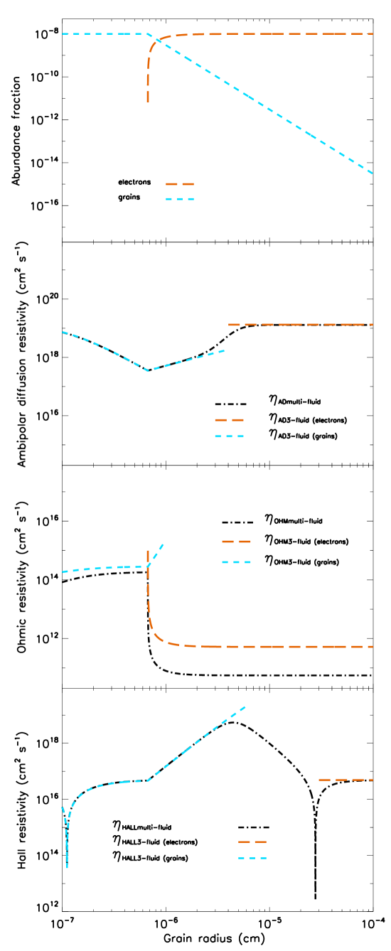
Figure 5: Values of $\eta_{\rm AD}$, $\eta_{\rm O}$ and $\eta_{\rm H}$ as function of the grain radius $r_{g}$ for conditions typical of a molecular cloud core (see text). The neutral, positive and negative species are H₂, HCO⁺, and electrons (long-dashed curves) or grains (short-dashed curves). The dash-dotted curves show the same quantities computed with the multi-fluid scheme.

In this section, we compare our results with those obtained by a multifluid scheme (arbitrary number of species, but only collisions with neutrals included). Neglecting Biermann’s battery and diamagnetic terms, Eq. (46) can be written in the standard form

$${\bf E}+\frac{{\bf U}}{c}\times{\bf B}=\left(\frac{1}{\sigma_{\parallel}}-\frac{\sigma_{\rm P}}{\sigma_{\rm P}^{2}+\sigma_{\rm H}^{2}}\right)\left[\frac{({\bf J}\times{\bf B})\times{\bf B}}{B^{2}}\right]$$ (107)

$$+\left(\frac{\sigma_{\rm H}}{\sigma_{\rm P}^{2}+\sigma_{\rm H}^{2}}\right)\frac{{\bf J}\times{\bf B}}{B}+\frac{\bf J}{\sigma_{\parallel}}$$

where $\sigma_{\parallel}$ is the conductivity parallel to the electric field, $\sigma_{\rm P}$ and $\sigma_{\rm H}$ are the Pedersen and Hall conductivities, respectively. The conductivities can be written in terms of the Hall parameters $\beta_{sn}$ defined as

$$\beta_{sn}=\left(\frac{q_{s}B}{m_{s}c}\right)\frac{\rho_{s}}{\alpha_{sn}}=\left(\frac{q_{s}B}{m_{s}c}\right)\frac{m_{s}+m_{n}}{\rho_{n}\langle\sigma v\rangle_{sn}}$$ (108)

the ratio of the cyclotron frequency of a particle $s$ and its characteristic frequency of collision with neutral particles (notice that the Hall parameter is negative for negatively-charged particles). From Eq. (46), the expressions of the conductivities result

$$\sigma_{\parallel}=\sigma(\beta_{+n}+|\beta_{-n}|),$$ (109)

$$\sigma_{\rm P}=\sigma\left(\frac{\beta_{+n}}{1+\beta_{+n}^{2}}+\frac{|\beta_{-n}|}{1+\beta_{-n}^{2}}\right)$$ (110)

$$\sigma_{\rm H}=\sigma\left(\frac{1}{1+\beta_{+n}^{2}}-\frac{1}{1+\beta_{-n}^{2}}\right)$$ (111)

where

$$\sigma=\frac{q_{+}\rho_{+}c}{m_{+}B}.$$ (112)

These expressions are a special case, for two charged fluids, of the general results of the multifluid approach,

$$\sigma_{\parallel}=\frac{c}{B}\sum_{s}\left(\frac{q_{s}\rho_{s}}{m_{s}}\right)\beta_{sn},$$ (113)

$$\sigma_{\rm P}=\frac{c}{B}\sum_{s}\left(\frac{q_{s}\rho_{s}}{m_{s}}\right)\frac{\beta_{sn}}{1+\beta_{sn}^{2}},$$ (114)

$$\sigma_{\rm H}=\frac{c}{B}\sum_{s}\left(\frac{q_{s}\rho_{s}}{m_{s}}\right)\frac{1}{1+\beta_{sn}^{2}}.$$ (115)

The corresponding resistivities are

$$\eta_{\rm AD}\equiv\frac{c^{2}}{4\pi}\left(\frac{\sigma_{\rm P}}{\sigma_{\rm P}^{2}+\sigma_{\rm H}^{2}}-\frac{1}{\sigma_{\parallel}}\right)=\left(\frac{c^{2}}{4\pi\sigma}\right)\frac{\beta_{+n}|\beta_{-n}|}{\beta_{+n}+|\beta_{-n}|}.$$ (116)

$$\eta_{\rm H}\equiv\frac{c^{2}}{4\pi}\left(\frac{\sigma_{\rm H}}{\sigma_{\rm P}^{2}+\sigma_{\rm H}^{2}}\right)=-\left(\frac{c^{2}}{4\pi\sigma}\right)\frac{\beta_{+n}-|\beta_{-n}|}{\beta_{+n}+|\beta_{-n}|},$$ (117)

$$\eta_{\rm O}\equiv\frac{c^{2}}{4\pi\sigma_{\parallel}}=\left(\frac{c^{2}}{4\pi\sigma}\right)\frac{1}{\beta_{+n}+|\beta_{-n}|}.$$ (118)

If the charged particles are electrons and ions, $m_{e}\ll m_{i}$. Since the collisional rate coefficient are of the same order for electron-neutral and ion-neutral collisions, in general $|\beta_{en}|\gg\beta_{in}$, and one has

$$\eta_{\rm H}=|\beta_{en}|\eta_{\rm O},\qquad\eta_{\rm AD}=|\beta_{en}|\beta_{in}\eta_{\rm O}.$$ (119)

As an illustration, we analyze the variation of the resistivities appearing in Eq. (47) as function of the grain size in a molecular cloud core.

Consider a molecular cloud core made of neutrals (H₂), ions (HCO⁺), electrons ($e$), and negatively -charged dust grains ($g^{-}$), with radius $r_{g}$. In particular, we assume $n_{n}=10^{6}$ cm^-3, $n_{i}=10^{-2}$ cm^-3, $\rho_{g}/\rho=0.01$, a temperature of $T=10$ K, and a magnetic field $B=0.1$ mG. Each grain is assumed to be spherical, with a radius $a$ varying between 10 Å and 0.1 mm, and mean interior density 2 g cm^-3. All grains are assumed to be negatively charged, and the number density of free electrons is obtained by the neutrality condition $n_{e}+n_{g^{-}}(r_{g})=n_{i}$. For high values of the grain’s radius, the number density of grains is small, and all the negative charge is carried by electrons. In the opposite limit, the number density of small grains is high, a fraction of the grain population is sufficient to carry all the negative charge, and the density of free electrons is zero.

References

- (1) Bacciotti, F., Eislöffel, J. 1999, A&A, 342, 717
- (2) Bacciotti, F., Eislöffel, J., Ray, T. P. 1999, A&A, 350, 917
- (3) Bacciotti, F., Ray, T. P., Mundt, R., Eislöffel, J., Sölf, J. 2002, ApJ, 576, 222
- (4) Benilov, M. S. 1996, Phys. Plasmas, 3, 2805
- (5) Benilov, M. S. 1997, Phys. Plasmas, 4, 521
- (6) Biermann, L. 1950, Z. f. Naturforschung, 5A, 65
- (7) Boyd, T. J., Sanderson, J. J. 1969, Plasma Dynamics (London: Nelson)
- (8) Braginskii, S. 1965, in Reviews of Plasma Physics, Vol. 1, M. Leontovich ed. (New York: Consultants Bureau), p. 205
- (9) Caselli, P., Walmsley, C. M., Tafalla, M., Dore, L., Myers, P. C. 1999, ApJ, 523, L165
- (10) Ciolek, G. E., Mouschovias, T. Ch. 1993, ApJ, 418, 774
- (11) Coffey, D., Bacciotti, F., Woitas, J., Ray, T. P., Eislöffel, J. 2004, ApJ, 604, 758
- (12) Coffey, D., Bacciotti, F., Ray, T. P., Eislöffel, J., Woitas, J. 2007, ApJ, 663, 350
- (13) Cowling, T. G. 1956, MNRAS, 116, 114
- (14) Desch, S. J., Mouschovias, T. Ch. 2001, ApJ, 550, 314
- (15) Draine, B. T., 1980, ApJ, 241, 1021
- (16) Draine, B. T. 1986, MNRAS, 220, 133
- (17) Draine, B. T., Roberge, W. G., Dalgarno, A. 1983, ApJ, 264, 485.
- (18) Draine, B. T., McKee, C. F. 1993, ARA&A, 31, 373
- (19) Dungey, J. W. 1958, Cosmic Electrodynamics (Cambridge: University Press)
- (20) Flower, D. R., Pineau des Forêts, G., Hartquist, T. W. 1985, MNRAS, 216, 775
- (21) Flower, D. R., Pineau des Forêts, G., Walmsley, C. M. 2005, A&A, 436, 933
- (22) Frank, A., Gardiner, T. A., Delemarter, G., Lery, T., Betti, R. 1999, ApJ, 524, 947
- (23) Galli, D., Shu, F. H. 1993a, ApJ, 417, 220
- (24) Galli, D., Shu, F. H. 1993b, ApJ, 417, 243
- (25) Garcia, P. J. V., Ferreira, J., Cabrit, S., Binette, L. 2001, A&A, 377, 589
- (26) Goldreich, P., Reisenegger, A. 1992, ApJ, 395, 250
- (27) Greene, J. M. 1973, Plasma Phys., 15, 29
- (28) Guillet, V., Pineau des Forêts, G., Jones, A. P. 2007, A&A, 476, 263
- (29) Hartigan, P., Morse, J. A., Raymond, J. 1994, ApJ, 436, 125
- (30) Hartigan, P., & Morse, J. 2007, Apj, 660, 426
- (31) Hartigan, P., Frank, A., Varniére, P., & Blackman, E. G. 2007, Apj, 661, 910
- (32) Kelley, M. C. 1989, The Earth’s Ionosphere: Plasma Physics & Electrodynamics (San Diego: Academic Press), p. 38
- (33) Krall, N. A., Trivelpiece, A. W., 1973, Principles of Plasma Physics (New York: McGraw-Hill)
- (34) Krtička, J., Kubát, J. 2001, A&A, 222, 238
- (35) Lazarian, A. 1992, A&A, 264, 326
- (36) Lizano, S., Shu, F. H. 1987, in Physical Processes in Interstellar Clouds, G. E. Morfill & M. Scholer eds. (Dordrecht: Kluwer)
- (37) Mestel, L., Spitzer, L. 1956, MNRAS, 116, 503
- (38) Mitchner, M., Kruger, C. H., 1973, Partially Ionized Gases (New York: Wiley Interscience)
- (39) Mouschovias, T. Ch. 1991, in The Physics of Star Formation and Early Stellar Evolution, C.J. Lada and N.D. Kylafis eds. (Dordrecht: Kluwer), p. 61
- (40) Mullan, D. J. 1971, MNRAS, 153, 145
- (41) Mundt, R., Buehrke, T., Solf, J., Ray, T. P., Raga, A. 1990, A&A, 232, 37
- (42) Nakano, T., Umebayashi, T. 1980, PASJ, 32, 613
- (43) Nakano, T., Umebayashi, T. 1986, MNRAS, 218, 663
- (44) Nakano, T., Nishi, R., Umebayashi, T. 2002, ApJ, 573, 199
- (45) Nakamura, F., Hanawa, T., Nakano, T. 1993, PASJ, 45, 551
- (46) Nishi, R., Nakano, T., Umebayashi, T. 1991, ApJ, 368, 181
- (47) Pandey, B. P., Wardle, M. 2007, astro-ph/0707.2688v1
- (48) Parks, G. K. 1991, Physics of Space Plasmas (Boulder: ABP Press)
- (49) Pineau des Forêts, G., Flower, D. R., Hartquist, T. W., Dalgarno, A. 1986, MNRAS, 220, 801
- (50) Pinto, C., Galli, D. 2007, A&A, submitted
- (51) Podio, C., Bacciotti, F., Nisini, B., Eislöffel, J., Massi, F., Giannini, T., & Ray, T. P. 2006, A&A, 456, 189
- (52) Ray, T. P., Muxlow, T. W. B., Axon, D. J., Brown, A., Corcoran, D., Dyson, J., Mundt, R. 1997, Nature, 385, 515
- (53) Reipurth, B., Bally, J. 2001, ARA&A, 39, 403
- (54) Rossi, B., Olbert, S. 1970, Introduction to the Physics of Space (New York: McGraw-Hill)
- (55) Ruden, S. P., Glassgold, A. E., Shu, F. H. 1990, ApJ, 361, 546
- (56) Safier, P. 1993, ApJ, 408, 115
- (57) Scalo, J. 1977, ApJ, 213, 705
- (58) Schlüter, A. 1950, Z. f. Naturforschung, 5A, 72
- (59) Schlüter, A. 1951, Z. f. Naturforschung, 6A, 73
- (60) Schlüter, A., Biermann, L. 1950, Z. f. Naturforschung, 5A, 237
- (61) Shang, Z., & Wills, B. 2004, AGN Physics with the Sloan Digital Sky Survey, 311, 13
- (62) Shu, F. H. 1983, ApJ, 273, 202
- (63) Spitzer, L. 1978, Physical Processes in the Interstellar Medium (New York: Wiley)
- (64) Tassis, K., Mouschovias, T. Ch. 2005, ApJ, 618, 769
- (65) Tohline, J. E. 1982, Fund. Cosm. Phys., 8, 1
- (66) Vasyliunas, V. M. 2005, Ann. Geophys., 23, 1347
- (67) Wardle, M. 1999, MNRAS, 307, 849
- (68) Wardle, M., Ng, C. 1999, MNRAS, 303, 239
- (69) Walmsley, C. M., Flower, D. R., Pineau des Forêts, G. 2004, A&A, 418, 1035
- (70) Weingartner, J. C., Draine, B. T. 2001, ApJS, 134, 263
- (71) Woitas, J., Bacciotti, F., Ray, T., Marconi, A., Coffey, D., Eislöffel, J. 2005, ApJ, 432, 149