Mixing effectiveness depends on the source-sink structure: Simulation results

Abstract

The mixing effectiveness, i.e., the enhancement of molecular diffusion, of a flow can be quantified in terms of the suppression of concentration variance of a passive scalar sustained by steady sources and sinks. The mixing enhancement defined this way is the ratio of the RMS fluctuations of the scalar mixed by molecular diffusion alone to the (statistically steady-state) RMS fluctuations of the scalar density in the presence of stirring. This measure of the effectiveness of the stirring is naturally related to the enhancement factor of the equivalent eddy diffusivity over molecular diffusion, and depends on the Péclet number. It was recently noted that the maximum possible mixing enhancement at a given Péclet number depends as well on the structure of the sources and sinks. That is, the mixing efficiency, the effective diffusivity, or the eddy diffusion of a flow generally depends on the sources and sinks of whatever is being stirred. Here we present the results of particle-based simulations quantitatively confirming the source-sink dependence of the mixing enhancement as a function of Péclet number for a model flow.

I Introduction

Mixing by fluid flows is a ubiquitous natural phenomenon that plays a central role in many of the applied sciences and engineering. A geophysical example is the mixing of aerosols (e.g., $\text{CO}_{2}$ supplied by a volcano, say, or by human activity) in the atmosphere. Aerosols are dispersed by molecular diffusion on the smallest scales but are more effectively spread globally by atmospheric flows. The density — and density fluctuations — of some aerosols influence the albedo of the earth and thus have a significant environmental impact. Hence it is important to understand fundamental properties of dispersion, mixing, and the reduction of concentration fluctuations by stirring flow fields.

Various aspects of mixing have been the focus of many review articles Ottino (1990); Majda and Kramer (1999); Warhaft (2000); Shraiman and Siggia (2000); Sawford (2001); Falkovich et al. (2001); Aref (2002); Wiggins and Ottino (2004). At the most basic level, the mixing of a passive scalar can be modeled by an advection-diffusion equation for the scalar concentration field with a specified stirring flow field. In this work we will focus on problems where fluctuations in the scalar field are generated and sustained by temporally steady but spatially inhomogeneous sources. The question of interest here is this: for a given source distribution, how well can a specified stirring flow mix the scalar field?

Mixing effectiveness can be measured by the scalar variance over the domain. A well-mixed scalar field will have a more uniform density with relatively “small” variance while increased fluctuations in the scalar density will be reflected in a “large” variance. We put quotes around the quantifiers small and large because the variance is a dimensional quantity that needs an appropriate dimensional point of reference from which it is being measured.

Several years ago Thiffeault et al Thiffeault et al. (2004) introduced a notion of “mixing enhancement” for a velocity field stirring a steadily sustained scalar by comparing the bulk (space-time) averaged density variance with and without advecting flow. Mixing is accomplished by molecular diffusion alone in the absence of stirring, which can be quite effective on small scales but is not generally so good at breaking up and dispersing large-scale fluctuations quickly. Stirring can greatly enhance the transport of the scalar from regions of excess density to depleted regions, suppressing the variance far below its diffusion-only value. The magnitude of this variance suppression by the stirring — the ratio of the variance without stirring to the variance in the presence of stirring — is a dimensionless quantity that provides a sensible gauge of the mixing effectiveness of the flow. Different advection fields will have different mixing efficiencies stirring scalars supplied by different sources. It is then of obvious interest both to determine theoretical limits on mixing enhancements for various source configurations and to explore whether those limits may be approached—or even perhaps achieved—-for particular flows.

There have been many studies of stirring and mixing of a scalar with fluctuations sustained by spatially inhomogeneous sources and sinks. Some of the earliest are by Townsend Townsend (1951, 1954), who was concerned with the effect of turbulence and molecular diffusion on a heated filament. He found that the spatial localization of the source enhanced the role of molecular diffusivity. Durbin Durbin (1980) and Drummond Drummond (1982) introduced stochastic particle models to turbulence modeling, and these allowed more detailed studies of the effect of the source on diffusion. Sawford and Hunt Sawford and Hunt (1986) pointed out that small sources lead to a dependence of the variance on molecular diffusivity. These models were further refined by Thomson (1990); Borgas and Sawford (1994); Sawford (2001). Chertkov et al Chertkov et al. (1995a, b, 1997); Chertkov (1997); Chertkov et al. (1998) and Balkovsky & Fouxon Balkovsky and Fouxon (1999) addressed the case of a random, statistically-steady source.

In this paper we study the enhancement of mixing by an advection field using a particle-based computational scheme that is easy to implement and applicable to a variety of source distributions. The idea is to develop a method that accurately simulates advection and diffusion of large numbers of particles supplied by a steady source, and to measure density fluctuations by “binning” the particles to produce an approximation of the hydrodynamic concentration field. Unlike a numerical PDE code, a particle code does not prefer specific forms of the flow or the source (PDE methods generally work best with very smooth fields). There is, however, no free lunch: the accuracy of the particle code is ultimately limited by the finite number of particles that can be tracked. The limitation to finite numbers of particles inevitably introduces statistical errors due to discrete fluctuations in the local density and systematic errors in the variance measurements due to binning. But these problems are tractable, and as we will show, the method proves to be quantitatively accurate and computationally efficient for some applications.

II Theoretical background

In this section we review basic facts about the mixing enhancement problem as formulated by Thiffeault, Doering & Gibbon et al Thiffeault et al. (2004) and developed by Plasting & Young Plasting and Young (2006), Doering & Thiffeault Doering and Thiffeault (2006), Shaw et al Shaw et al. (2007), and Thiffeault and Pavliotis Thiffeault and Pavliotis (2008). The dynamics is given by the advection-diffusion equation for the concentration of a passive scalar $\rho(t,\bm{x})$ with time-independent but spatially inhomogeneous source field $S(\bm{x})$:

$$\frac{\partial\rho}{\partial t}+\bm{u}\cdot\nabla\rho=\kappa\Delta\rho+S(\bm{x}),$$ (1)

where $\kappa$ is the molecular diffusivity and $\bm{u}(t,\bm{x})$ is a specified advection field that satisfies (at each instant of time) the incompressibility condition

$$\nabla\cdot\bm{u}=0.$$ (2)

For simplicity, the domain is the $d$-torus, i.e., $[0,L]^{d}$ with periodic boundary conditions. We limit attention to stirring fields that satisfy the properties of statistical homogeneity and isotropy in space defined by

$$\overline{u_{i}(\cdot,\bm{x})}=0,\qquad\overline{u_{i}(\cdot,\bm{x})u_{j}(\cdot,\bm{x})}=\frac{U^{2}}{d}\delta_{ij}$$ (3)

where the overbar denotes time-averaging and $U$ is the root mean square speed of the velocity field, a natural indicator of the intensity of the stirring. These are statistical properties of homogeneous isotropic turbulence on the torus, but they are also shared by many other kinds of flows.

We are interested in fluctuations in the concentration $\rho$ so the spatially averaged background density is irrelevant. It is easy to see from (1) that the spatial average of $\rho$ grows linearly with time at the rate given by the spatial average of $S$. Hence we change variables to spatially mean-zero quantities

$$\theta(t,\bm{x})=\rho(t,\bm{x})-\frac{1}{L^{d}}\int\mathrm{d}^{d}x^{\prime}\,\rho(t,\bm{x}^{\prime})$$ (4)

and

$$s(\bm{x})=S(\bm{x})-\frac{1}{L^{d}}\int\mathrm{d}^{d}x^{\prime}\,S(\bm{x}^{\prime})$$ (5)

that satisfy

$$\frac{\partial\theta}{\partial t}+\bm{u}\cdot\nabla\theta=\kappa\Delta\theta+s(\bm{x}).$$ (6)

(We must also supply initial conditions for $\rho$ and/or $\theta$ but they play no role in the long-time steady statistics that we are interested in.)

The “mixedness” of the scalar may be characterized by, among other quantities, the long-time averaged variance of $\rho$, proportional to the long-time averaged $L^{2}$ norm of $\theta$,

$$\langle\theta^{2}\rangle:=\lim_{T\to\infty}\frac{1}{T}\int_{0}^{T}\mathrm{d}t\ \frac{1}{L^{d}}\int\mathrm{d}^{d}x\,\theta^{2}(t,\bm{x})$$ (7)

The smaller $\langle\theta^{2}\rangle$ is, the more uniform the distribution. The “mixing enhancement” of a stirring field is naturally measured by comparing the scalar variance to the variance with the same source but in the absence of stirring. To be precise, we compare $\langle\theta^{2}\rangle$ to $\langle\theta_{0}^{\ 2}\rangle$ where $\theta_{0}$ is the solution to

$$\frac{\partial\theta_{0}}{\partial t}=\kappa\Delta\theta_{0}+s(\bm{x})$$ (8)

(with, say, the same initial data although these will not affect the long-time averaged fluctuations). The dimensionless mixing enhancement factor is then defined as

$${\cal E}_{0}:=\sqrt{\frac{\langle\theta_{0}^{\,2}\rangle}{\langle\theta^{2}\rangle}}.$$ (9)

This quantity carries the subscript $0$ because we can also define multiscale mixing enhancements Doering and Thiffeault (2006); Shaw et al. (2007) by weighting large/small wavenumber components of the scalar fluctuations:

$${\cal E}_{p}:=\sqrt{\frac{\langle|\nabla^{p}\theta_{0}|^{2}\rangle}{\langle|\nabla^{p}\theta|^{2}\rangle}}\,,\qquad p=-1,0,1.$$ (10)

As discussed in Doering & Thiffeault Doering and Thiffeault (2006), Shaw et al Shaw et al. (2007) and Shaw Shaw (2005), ${\cal E}_{\pm 1}$ provide a gauge of the mixing enhancement of the flow as measured by scalar fluctuations on relatively small and large length scales, respectively. We refer to them as enhancement factors because if one were to define an effective, eddy, or equivalent diffusivity $\kappa_{e,p}$ as the value of a molecular diffusion necessary to produce the same value of $\langle|\nabla^{p}\theta|^{2}\rangle$ with stirring, then $\kappa_{e,p}=\kappa{\cal E}_{p}$. In this paper, however, we will focus exclusively on ${\cal E}_{0}$, the mixing enhancement at “moderate” length scales.

There is a theoretical upper bound on ${\cal E}_{0}$ valid for any statistically stationary homogeneous and isotropic stirring field Doering and Thiffeault (2006); Shaw (2005); Shaw et al. (2007):

$${\cal E}_{0}\leq\sqrt{\frac{\sum_{\bm{k}\neq\bm{0}}|\hat{s}(\bm{k})|^{2}/k^{4}}{\sum_{\bm{k}\neq\bm{0}}|\hat{s}(\bm{k})|^{2}/(k^{4}+\frac{{\rm Pe}^{2}}{L^{2}d}k^{2})}}$$ (11)

where $\hat{s}(\bm{k})$ are the Fourier coefficients of the source and the Péclet number,

$${\rm Pe}:={UL}/{\kappa},$$ (12)

is a dimensionless measure of the intensity of the stirring. Generally, we anticipate that ${\cal E}_{0}$ is an increasing function of Pe and the estimate in (11) guarantees that ${\cal E}_{0}(\text{Pe})\lesssim\text{Pe}$ as $\text{Pe}\rightarrow\infty$, the “classical” scaling necessary if there is to be any residual variance suppression in the singular vanishing diffusion limit. That is, if ${\cal E}_{0}(\text{Pe})\sim\text{Pe}$ then $\kappa_{e,0}$ has a nonzero limit as $\kappa\rightarrow 0$ with all other parameters held fixed. It is natural to refer to any of the possible sub-classical scalings as “anomalous”.

The upper limit to the mixing enhancement in (11) depends on the stirring field only through $U$ via Pe, but it depends on all the details of the source distribution. As studied in depth in references Doering and Thiffeault (2006); Shaw et al. (2007); Shaw (2005), the structure of the scalar source can have a profound effect on the high Pe scaling of ${\cal E}_{0}$, notably for sources with small scales. It is physically meaningful to consider measure-valued source-sink distributions, like delta-functions, with arbitrarily small scales. It is precisely this source size dependence of ${\cal E}_{0}(\text{Pe})$ that motivates the development of a computational method that can handle singular source distributions.

In this study, for computational simplicity and efficiency, we utilize the “random sine flow” as the stirring field. In the two-dimensional case this is defined for all time by

$${\bm{u}}(t,\bm{x})=\begin{cases}w\sin\left({2\pi y}/{L}+\phi\right)\hat{\textbf{\i}}\,,\qquad&nT<t\leq nT+\tfrac{1}{2}T;\\ w\sin\left({2\pi x}/{L}+\phi^{\prime}\right)\hat{\textbf{\j}}\,,\qquad&nT+\tfrac{1}{2}T<t\leq(n+1)T,\end{cases}$$ (13)

where $T$ is the period, $n=0,1,2,\dots$, and $\phi$ and $\phi^{\prime}$ are random phases chosen independently and uniformly on $[0,2\pi)$ in each half cycle, which assures the homogeneity of the flow field. In this case, $w=\sqrt{2}U$. In the three-dimensional case, we employ

$$\bm{u}(t,\bm{x})=\begin{cases}w\left[\sin\alpha\sin\left(2\pi y/L+\phi_{2}\right)+\cos\alpha\sin\left(2\pi z/L+\phi_{3}\right)\right]\hat{\textbf{\i}}\,,\ &nT<t\leq nT+\tfrac{1}{3}T;\\ w\left[\sin\alpha\sin\left(2\pi z/L+\psi_{3}\right)+\cos\alpha\sin\left(2\pi x/L+\phi_{1}\right)\right]\hat{\textbf{\j}}\,,\ &nT+\tfrac{1}{3}T<t\leq nT+\tfrac{2}{3}T;\\ w\left[\sin\alpha\sin\left(2\pi x/L+\psi_{1}\right)+\cos\alpha\sin\left(2\pi y/L+\psi_{2}\right)\right]\hat{\textbf{k}}\,,\ &nT+\tfrac{2}{3}T<t\leq(n+1)T,\end{cases}$$

where again $w=\sqrt{2}U$, $n=0,1,2,\dots$, and $\alpha$, $\phi_{1,2,3}$ and $\psi_{1,2,3}$ are uniform random numbers in $[0,2\pi)$ chosen independently every $T/3$. The angle $\alpha$ randomizes the shear direction to guarantee isotropy of the flow.

III Numerical method

In a particle code for solving the advection-diffusion equation, the concentration field $\rho$ is represented by a distribution of particles. Particles are introduced by generating random locations using the properly normalized source $S(\bm{x})$ as a probability distribution function, then they are transported by advection and diffusion. The particle density, $\rho(t,\bm{x})$, is measured by covering the domain with bins counting the number of particles per bin.

A discrete particle method is employed because it can easily deal with small-scale sources such as $\delta$ functions. It is also straightforward to implement with any advection field. The downside of a particle method is that it necessarily involves two kinds of errors: the number density of particles calculated by dividing the domain into bins is only resolved down to the size of the bins, and the measurement of $\rho$ always includes statistical errors due to the use of finite numbers of particles.

III.1 Time evolution

At each time step the system is evolved by advection, diffusion, the source, and sinks. An advection-only equation would be solved by moving particles along characteristics, and a diffusion-only equation would be solved by adding independent Gaussian noises to each coordinate of each particle. With both advection and diffusion we need to solve a stochastic differential equation to determine the proper displacement of the particles during a time step. The stochastic differential equation is

$$d\bm{X}=\bm{u}(t,\bm{X})dt+\sqrt{2\kappa}\ d\bm{W}$$ (14)

where $\bm{W}(t)$ is a standard vector-valued Wiener process.

In order to solve (14), we will consider cases where the displacement due to the noise in a subinterval of length $T/d$ (where $d$ is the dimension) is much smaller than the wavelength of the random sine flow. This condition is realized better and better as Pe increases. Then, during each subinterval, the drift field $\bm{u}(t,\bm{X})$ experienced by each particle can be approximated by a steady flow with a linear shear. In 2D, for the first half of the period for a particle starting at $(x_{0},y_{0})=(X(t=0),Y(t=0))$ we approximate (14) by

$$\begin{split}dX&=w\sin\left({2\pi y_{0}}/{L}+\phi\right)dt+w\cos\left({2\pi y_{0}}/{L}+\phi\right)\dfrac{2\pi}{L}(Y-y_{0})dt+\sqrt{2\kappa}\,dW_{1},\\ dY&=\sqrt{2\kappa}\,dW_{2},\end{split}$$ (15)

and for the second half of the period, starting from $(x^{\prime}_{0},y^{\prime}_{0})=(X(t=T/2),Y(t=T/2))$,

$$\begin{split}dX&=\sqrt{2\kappa}\,dW_{1},\\ dY&=w\sin\left({2\pi x^{\prime}_{0}}/{L}+\phi^{\prime}\right)dt+w\cos\left({2\pi x^{\prime}_{0}}/{L}+\phi^{\prime}\right)\dfrac{2\pi}{L}(X-x^{\prime}_{0})dt+\sqrt{2\kappa}\,dW_{2}\,.\end{split}$$ (16)

Therefore, during the first half period we evolve the position of a particle through a time interval $\Delta t$ (where $\Delta t\leq T/2$ need not be small) by the map

$$\begin{split}x_{0}&\rightarrow x_{0}+w\sin\left({2\pi y_{0}}/{L}+\phi\right)\Delta t+R_{1},\\ y_{0}&\rightarrow y_{0}+R_{2},\end{split}$$ (17)

where $R_{1}$ and $R_{2}$ satisfy

$$\begin{split}dR_{1}&=S_{2}R_{2}dt+\sqrt{2\kappa}dW_{1}\qquad\left(S_{2}:=2\pi wL^{-1}\cos\left({2\pi y_{0}}/{L}+\phi\right)\right),\\ dR_{2}&=\sqrt{2\kappa}dW_{2}.\end{split}$$ (18)

The variance-covariance matrix of $R_{1}$ and $R_{2}$ is

$$\left(\begin{array}[]{cc}\bm{E}(R_{1}^{\ 2})&\bm{E}(R_{1}R_{2})\\ \bm{E}(R_{2}R_{1})&\bm{E}(R_{2}^{\ 2})\\ \end{array}\right)=\left(\begin{array}[]{cc}\frac{2}{3}S_{2}^{\ 2}\kappa t^{3}+2\kappa t&S_{2}\kappa t^{2}\\ S_{2}\kappa t^{2}&2\kappa t\\ \end{array}\right),$$ (19)

which is realized by

$$R_{1} =\sqrt{\tfrac{1}{6}S_{2}^{\ 2}\kappa t^{3}+2\kappa t}\times N_{1}+\sqrt{\tfrac{1}{2}S_{2}^{\ 2}\kappa t^{3}}\times N_{2},$$ (20)

$$R_{2} =\sqrt{2\kappa t}\times N_{2},$$ (21)

where $N_{1}$ and $N_{2}$ are independent $N(0,1)$ random variables (normally distributed with mean $0$ and standard deviation $1$). The matrix (19) describes the evolution of a passive scalar field in a shear flow Taylor (1954); Aris (1956); Rhines and Young (1983).

Therefore the time evolution map during the first half period is

$$x_{0} \rightarrow x_{0}+w\sin\left({2\pi y_{0}}/{L}+\phi\right)\,\Delta t+\sqrt{\tfrac{1}{6}S_{2}^{\ 2}\kappa(\Delta t)^{3}+2\kappa\Delta t}\,N_{1}+\sqrt{\tfrac{1}{2}S_{2}^{\ 2}\kappa(\Delta t)^{3}}\,N_{2}\,,$$ (22a)

$$y_{0} \rightarrow y_{0}+\sqrt{2\kappa\Delta t}\,N_{2}\,.$$ (22b)

A similar map is employed during the second half of the period. These stochastic maps include the shear — in the approximation that the shear remains constant for each particle during each half cycle — that causes a “distortion” of a Gaussian cloud of particles; see Fig. 1.

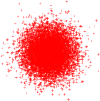
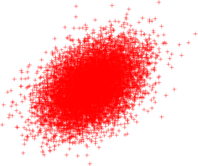
Figure 1: (a) A circular Gaussian distribution of particles transported and sheared into (b) an elliptical Gaussian cloud.

The same calculations apply for the three-dimensional case: for the first subinterval, the time-evolution map is

$$x_{0} \rightarrow x_{0}+w\left[\sin\alpha\sin\left({2\pi y_{0}}/{L}+\phi_{2}\right)+\cos\alpha\sin\left({2\pi z_{0}}/{L}+\phi_{3}\right)\right]$$

$$\phantom{\rightarrow x_{0}}+\sqrt{\tfrac{1}{6}(S_{2}^{\ 2}+S_{3}^{\ 2})\kappa(\Delta t)^{3}+2\kappa\Delta t}\,N_{1}+S_{2}\sqrt{\tfrac{1}{2}\kappa}(\Delta t)^{\frac{3}{2}}\,N_{2}+S_{3}\sqrt{\tfrac{1}{2}\kappa}(\Delta t)^{\frac{3}{2}}\,N_{3},$$ (23a)

$$y_{0} \rightarrow y_{0}+\sqrt{2\kappa\Delta t}\,N_{2},$$ (23b)

$$z_{0} \rightarrow z_{0}+\sqrt{2\kappa\Delta t}\,N_{3},$$ (23c)

where $S_{2}=2\pi wL^{-1}\sin\alpha\cos({2\pi y_{0}}/{L}+\phi_{2})$, $S_{3}=2\pi wL^{-1}\cos\alpha\cos({2\pi z_{0}}/{L}+\phi_{3})$, and $N_{1},N_{2}$ and $N_{3}$ are independent $N(0,1)$ random variables. The maps for the other subintervals can be obtained by cyclic permutation of the coordinates.

The steady scalar source is realized by introducing a new particle one by one using normalized $S(\bm{x})$ as a probability distribution function. Numerically, such a probability distribution function can be realized by mapping uniform random numbers over $[0,1]$ with the inverse of the cumulative probability distribution function in question.

New particles are added constantly so the total number of particles continues to increase, which slows down the computation. To cope with increasing particles, we implement a particle subtraction scheme. Particles eventually get well mixed and “older” particles do not contribute to the value of the hydrodynamic variance. There is no added value in keeping track of particles that have been in the mix for a very long time, and we can simply remove them from the system after a sufficiently long time. It is very important to keep track of the “age” of each particle, however, and to only remove sufficiently old well-mixed particles. (For example, if a random fraction of particles is removed at regular time intervals, then the simulation becomes one of a system particles with a random finite lifetime, described by an advection-diffusion equation with an additional density decay term.)

In order to determine how old particles must be in order to safely remove them without affecting the hydrodynamic variance, prior to a full simulation run a test is performed as follows. Starting from an initial set of $N_{i}$ particles located in space according to the source distribution, the flow and diffusion are allowed to act and the variance of the number of particles per bin, which decays with time, is monitored. The number $N_{i}$ is of the order of the number of particles that are introduced in the full simulation during, say, an interval of length $T$ characteristic of the random sine flow. The variance does not decay all the way to zero, however, but rather to the variance expected when $N_{i}$ particles are randomly distributed among the bins. The time when the variance achieves this random-distribution variance, measured beforehand for a given flow and diffusion strength, is then the required “aging” time before particles can be safely removed in the full simulation with the steady source. Such a trial run is performed for each flow, diffusion strength, source distribution and particle number because this “mixing time” depends on all these factors. Futher details of the criteria for removing old particles and extensive tests and benchmark trials may be found in Ref. Okabe (2006).

III.2 Variance calculation and background noise

The variance $\langle\theta^{2}\rangle$ is measured by monitoring the fluctuations in the number of particles per bin, and time-averaging. In $d$ dimensions the domain is divided into $l^{d}$ bins and the code calculates $\langle n^{2}\rangle$, where $n$ is the number of particles in a bin. Then $\langle\theta^{2}\rangle$ is initially approximated by

$$\langle n^{2}\rangle-\langle n\rangle^{2}=\left(L/l\right)^{2d}\langle\theta^{2}\rangle.$$ (24)

We say “initially” because the expression above includes both the hydrodynamic fluctuations of interest and discreteness fluctuations resulting solely from the fact that each bin contains a finite number of particles.

The subtraction scheme eliminates the “well-mixed” particles that do not contribute to the value of the hydrodynamic variance. But even if the system were completely mixed so that theoretically, $\langle\theta^{2}\rangle=0$, the measured variance $\langle n^{2}\rangle-\langle n\rangle^{2}$ would be (very close to, for small bins) $\langle n\rangle$, which is on the order of $N/l^{d}$, where $N$ is the total number of particles in the domain. This follows from the fact that $\theta(t,\bm{x})$ is represented in this particle method by only a finite number of particles in each finite size bin. That is, $\langle\theta^{2}\rangle$ as defined by (24) is nonzero even when the particles are uniformly distributed: then the bulk variance includes fluctuations as if $N$ particles were randomly thrown in $l^{d}$ bins. The helpful fact is that the bulk variance contribution from these background fluctuations due to finite numbers of particles in the bins does not depend on (i.e., is uncorrelated with) the hydrodynamic density variation from bin to bin. The total contribution to the variance is the sum of the “extra” variance in each bin which is linear in the (mean) number of particles in each bin. Hence the sum of the variances is $\sim N$ and the bulk variance contribution from the background fluctuations, $Nl^{d}/L^{2d}$, can simply be subtracted from the initial estimate for $\langle\theta^{2}\rangle$ in (24). The net result is our measured value of the hydrodynamic variance.

In addition to the inevitable fluctuations due to discreteness, density variations are observed only down to the length scales $\sim L/l$ because of the binning density, which is another source of error in this procedure. We use $l\geq 100$, which tests and benchmark studies indicate is sufficient for the examples studies here Okabe (2006).

The variance is calculated once for each subinterval, and the instant when it is calculated is determined randomly in order to obtain an unbiased time average. Thus each subinterval is divided into two parts, before and after variance calculation, and the particle transport and source processes are appropriately adapted. The final measured quantities are long time averages that are observed to be converged to within the error indicated on the plots below.

IV Results

In order to investigate the effect of source-sink scales on maximal and actual mixing enhancements, we performed a series of simulations for square-shaped sources of various sizes $a<L$ as illustrated in Fig. 2.

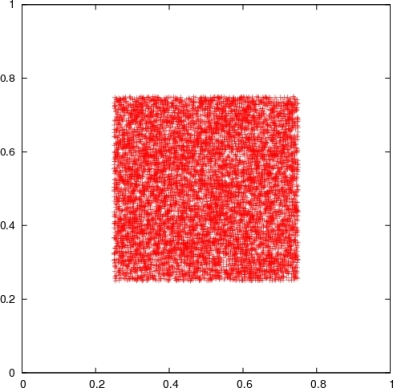
(a)  $a=L/2$

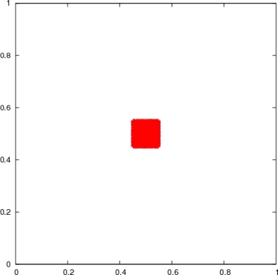
(b)  $a=L/10$

Figure 2: Square-shaped source of two different sizes; particles shown sampled from the uniform source distribution over the squares.

Fig 3(a) shows the upper bounds on ${\cal E}_{0}$ for square sources and a $\delta$-function source in 2D computed from (11). The upper bound for any finite-size source is asymptotically $\sim$ Pe, but for the $\delta$-function source it is $\sim{\rm Pe}/\ln{\rm Pe}$ in the large Pe limit. In 3D, the distinction between cubic sources and a $\delta$-function source is more apparent as shown in Fig 3(b): the upper bound for a $\delta$-function source behaves $\sim\sqrt{{\rm Pe}}$ in 3D. We stress that these mixing enhancement bounds apply for any statistically homogeneous and isotropic flows stirring sources with these shapes.

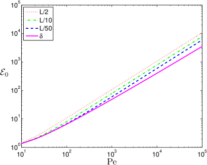
(a)  $d=2$

(b)  $d=3$

Figure 3: The theoretical upper bounds for (a) square sources with sizes $a=L/2,L/10,L/50$, and a $\delta$-function source; (b) cubic sources with sizes $a=L/5,L/50,L/500$, and a $\delta$-function source (from top to bottom).

Simulation results for the random sine flow, shown in Fig. 4(a) for 2D and Fig. 4(b) for 3D qualitatively confirm the behavior of the enhancements suggested by the upper limits. As the source size shrinks, the measured mixing enhancement gets smaller in a way that is remarkably similar to the bounds. In these simulations Pe is varied by decreasing $\kappa$ at a fixed values of $L,U$ and $T$. Other values of $T$ and other (shorter) wavelengths of the stirring flow were also checked, producing similar plots. These 2D simulation results have recently been confirmed quantitatively by a PDE computation Chertock et al. (2008).

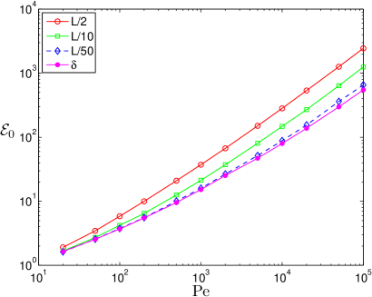
(a)  $d=2$

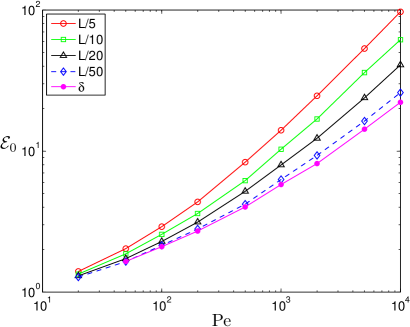
(b)  $d=3$

Figure 4: Measured mixing enhancements for (a) square sources with sizes $a=L/2,L/10,L/50$ and a $\delta$-function source, (b) cubic sources with sizes $a=L/5,L/50,L/500$ and a $\delta$-function source (from top to bottom).

The simulations also show that the upper estimates can give the correct quantitative behavior of ${\cal E}_{0}$ as a function of Pe. Indeed, in Fig 5 we plot the upper bound on ${\cal E}_{0}$ for the $\delta$-function source in 3D and the measured enhancement from the simulations. The upper bound, which scales anomalously $\sim\sqrt{{\rm Pe}}$, is an excellent predictor of the data. From this we conclude that the random sine flow is an “almost-optimal” mixer (among statistically homogeneous and isotropic flows) for this source-sink distribution.

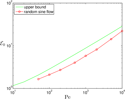
Figure 5: Mixing enhancement for a $\delta$-function source. The solid line is the upper bound for any SHI flow and the data are mixing enhancements for the random sine flow measured in the discrete particle simulations.

V Summary and conclusions

We have devised an accurate and computationally efficient particle method to study hydrodynamic variance suppression by a mixing flow. Rigorous upper bounds for the mixing enhancement ${\cal E}_{0}$, i.e., the effective diffusion enhancement factor, were compared to measured enhancements for the simple random sine flow. A key prediction of the analysis in Refs. Doering and Thiffeault (2006); Shaw et al. (2007) is that the source-sink shape is a determining factor in the mixing enhancement of any flow. The simulation results reported here show that the upper estimates give the correct qualitative picture as regards the Pe and source-shape dependence of ${\cal E}_{0}$.

Future work should focus on investigating enhancements of other stirring flows. No attempt has been made here to find a more efficient stirring flow (or, indeed, the most efficient flow, if there is one) whose enhancement approaches more closely (or perhaps even saturates) the upper bound. It is remarkable that the simple random sine flow appears to saturate the upper bound scaling ${\cal E}_{0}\sim\sqrt{{\rm Pe}}$ in 3D.

Stirring with appropriate turbulent solutions to the Navier–Stokes equation is also of significant interest. The central question here is, is statistically homogeneous and isotropic turbulence generically an efficient mixer? The answer may depend on the source-sink distribution.

References

- Ottino (1990) J. M. Ottino, ‘Mixing, chaotic advection, and turbulence,’ Annu. Rev. Fluid Mech. 22, 207–253 (1990).
- Majda and Kramer (1999) A. J. Majda and P. R. Kramer, ‘Simplified models for turbulent diffusion: Theory, numerical modelling and physical phenomena,’ Physics Reports 314 (4-5), 237–574 (1999).
- Warhaft (2000) Z. Warhaft, ‘Passive scalars in turbulent flows,’ Annu. Rev. Fluid Mech. 32, 203–240 (2000).
- Shraiman and Siggia (2000) B. I. Shraiman and E. D. Siggia, ‘Scalar turbulence,’ Nature 405, 639–646 (2000).
- Sawford (2001) B. L. Sawford, ‘Turbulent relative dispersion,’ Annu. Rev. Fluid Mech. 33, 289–317 (2001).
- Falkovich et al. (2001) G. Falkovich, K. Gawȩdzki, and M. Vergassola, ‘Particles and fields in turbulence,’ Rev. Mod. Phys. 73 (4), 913–975 (2001).
- Aref (2002) H. Aref, ‘The development of chaotic advection,’ Phys. Fluids 14 (4), 1315–1325 (2002).
- Wiggins and Ottino (2004) S. Wiggins and J. M. Ottino, ‘Foundations of chaotic mixing,’ Phil. Trans. R. Soc. Lond. A 362, 937–970 (2004).
- Thiffeault et al. (2004) J.-L. Thiffeault, C. R. Doering, and J. D. Gibbon, ‘A bound on mixing efficiency for the advection–diffusion equation,’ J. Fluid Mech. 521, 105–114 (2004).
- Townsend (1951) A. A. Townsend, ‘The diffusion of heat spots in isotropic turbulence,’ Proc. R. Soc. Lond. A 209 (1098), 418–430 (1951).
- Townsend (1954) A. A. Townsend, ‘The diffusion behind a line source in homogeneous turbulence,’ Proc. R. Soc. Lond. A 224 (1159), 487–512 (1954).
- Durbin (1980) P. A. Durbin, ‘A stochastic model of two-particle dispersion and concentration fluctuations in homogeneous turbulence,’ J. Fluid Mech. 100, 279–302 (1980).
- Drummond (1982) I. T. Drummond, ‘Path-integral methods for turbulent diffusion,’ J. Fluid Mech. 123, 59–68 (1982).
- Sawford and Hunt (1986) B. L. Sawford and J. C. R. Hunt, ‘Effects of turbulence structure, molecular diffusion and source size on scalar fluctuations in homogeneous turbulence,’ J. Fluid Mech. 165, 373–400 (1986).
- Thomson (1990) D. J. Thomson, ‘A stochastic model for the motion of particle pairs in isotropic high-Reynolds number turbulence, and its application to the problem of concentration variance,’ J. Fluid Mech. 210, 113–153 (1990).
- Borgas and Sawford (1994) M. S. Borgas and B. L. Sawford, ‘A family of stochastic models for two-particle dispersion in isotropic homogeneous stationary turbulence,’ J. Fluid Mech. 279, 69–99 (1994).
- Chertkov et al. (1995a) M. Chertkov, G. Falkovich, I. Kolokolov, and V. Lebedev, ‘Statistics of a passive scalar advected by a large-scale two-dimensional velocity field: Analytic solution,’ Phys. Rev. E 51 (6), 5609–5627 (1995a).
- Chertkov et al. (1995b) M. Chertkov, G. Falkovich, I. Kolokolov, and V. Lebedev, ‘Normal and anomalous scaling of the fourth-order correlation function of a randomly advected passive scalar,’ Phys. Rev. E 52 (5), 4924–4941 (1995b).
- Chertkov et al. (1997) M. Chertkov, I. Kolokolov, and M. Vergassola, ‘Inverse cascade and intermittency of passive scalar in one-dimensional smooth flow,’ Phys. Rev. E 56 (5), 5483–5499 (1997).
- Chertkov (1997) M. Chertkov, ‘Instanton for random advection,’ Phys. Rev. E 55 (3), 2722–2735 (1997).
- Chertkov et al. (1998) M. Chertkov, G. Falkovich, and I. Kolokolov, ‘Intermittent dissipation of a passive scalar in turbulence,’ Phys. Rev. Lett. 80 (10), 2121–2124 (1998).
- Balkovsky and Fouxon (1999) E. Balkovsky and A. Fouxon, ‘Universal long-time properties of Lagrangian statistics in the Batchelor regime and their application to the passive scalar problem,’ Phys. Rev. E 60 (4), 4164–4174 (1999).
- Plasting and Young (2006) S. Plasting and W. R. Young, ‘A bound on scalar variance for the advection–diffusion equation,’ J. Fluid Mech. 552, 289–298 (2006).
- Doering and Thiffeault (2006) C. R. Doering and J.-L. Thiffeault, ‘Multiscale mixing efficiencies for steady sources,’ Phys. Rev. E 74 (2), 025301(R) (2006).
- Shaw et al. (2007) T. A. Shaw, J.-L. Thiffeault, and C. R. Doering, ‘Stirring up trouble: Multi-scale mixing measures for steady scalar sources,’ Physica D 231 (2), 143–164 (2007).
- Thiffeault and Pavliotis (2008) J.-L. Thiffeault and G. A. Pavliotis, ‘Optimizing the source distribution in fluid mixing,’ Physica D (2008), in press, eprint http://dx.doi.org/10.1016/j.physd.2007.11.013.
- Shaw (2005) T. A. Shaw, ‘Bounds on multiscale mixing efficiencies,’ in Proceedings of the 2005 Summer Program in Geophysical Fluid Dynamics, 291 (Woods Hole Oceanographic Institute, Woods Hole, MA, 2005), eprint http://www.whoi.edu/cms/files/Shaw_21281.pdf.
- Taylor (1954) G. I. Taylor, ‘The dispersion of matter in turbulent flow through a pipe,’ Proc. R. Soc. Lond. A 223 (1155), 446–468 (1954).
- Aris (1956) R. Aris, ‘On the dispersion of a solute in a fluid flowing through a tube,’ Proc. R. Soc. Lond. A 235 (1200), 67–77 (1956).
- Rhines and Young (1983) P. B. Rhines and W. R. Young, ‘How rapidly is a passive scalar mixed within closed streamlines?’ J. Fluid Mech. 133, 133–145 (1983).
- Okabe (2006) T. Okabe, ‘A particle-simulation method to study mixing efficiencies,’ in Proceedings of the 2006 Summer Program in Geophysical Fluid Dynamics (Woods Hole Oceanographic Institute, Woods Hole, MA, 2006), eprint http://www.whoi.edu/cms/files/Taka_21241.pdf.
- Chertock et al. (2008) A. Chertock, E. Kashdan, A. Kurganov, and C. Doering, ‘A fast explicit operator splitting method for passive scalar advection by a random stirring field,’ (2008), in preparation.