Bivariate phase-rectified signal averaging
Abstract
Phase-Rectified Signal Averaging (PRSA) was shown to be a powerful tool for the study of quasi-periodic oscillations and nonlinear effects in non-stationary signals. Here we present a bivariate PRSA technique for the study of the inter-relationship between two simultaneous data recordings. Its performance is compared with traditional cross-correlation analysis, which, however, does not work well for non-stationary data and cannot distinguish the coupling directions in complex nonlinear situations. We show that bivariate PRSA allows the analysis of events in one signal at times where the other signal is in a certain phase or state; it is stable in the presence of noise and impassible to non-stationarities.
keywords:
Time-series analysis; Quasi-periodicities; Non-stationaritiy behavior; Cross-correlation analysis; Phase-rectified signal averagingPACS: 05.40.a; 05.45.Tp; 02.50.Sk; 87.19.Hh
, , and
1 Introduction
Many natural systems generate periodicities on different time scales because some of their components form closed regulation loops in addition to causal linear control chains. In biology and physiology, cardio-respiratory rhythms, rhythmic motions of limbs in walking, rhythms underlying the release of hormones and gene expression, membrane potential oscillations, oscillations in neuronal signals, and circadian rhythms are just a few examples (see, e.g., [1, 2]). Oscillations also occur in geophysical data, e.g., for the El-Niño phenomenon, sunspot numbers, and ice age periods [3]. In many cases several signals from different components of the complex system can be recorded simultaneously. For understanding the control chains and loops in the system, we want to know how periodicities in the signals are generated by (possibly directed and/or nonlinear) interactions between its components. Consequently, there is a need for identifying periodicities in one recorded signal together with the direction of causal relations to periodicities in other signals.
Cross-correlation analysis and transfer function analysis are traditional tools for this type of analysis. However, there are three major drawbacks of these methods: (i) only rather stationary data can be studied, (ii) a linear relationship between the signals is usually assumed, and (iii) the identification of causalities is hindered by the fact that the exchange of the two signals under study is identical with time inversion. We thus propose a method which helps to overcome these problems.
Non-stationarities are a major problem in the analysis of signals recorded from complex systems over a prolonged period of time [4, 5, 6, 7, 8]. Many internal and external perturbations are continuously influencing the system and causing interruptions of the periodic behavior. The interruptions often ’reset’ the regulatory mechanisms resulting in phase de-synchronization of the oscillations. The signals thus become quasi-periodic, consisting of many periodic patches as well as noise and trends. Cross-correlation and transfer function techniques are thus problematic. In addition, there might be causal inter-relations between two signals that cannot be revealed by these methods. For illustration, let us assume that a large increase and a large decrease in signal (trigger signal) cause the same specific effect in signal (target signal), while there is no such effect in if remains unchanged. In this situation with an essentially nonlinear coupling between the signals, both, cross-correlation analysis and spectral analysis cannot reveal the effect. They show the superposition of the two branches of the interaction with opposite signs, i.e., no effect. Even if the effects on signal were different for increases and decreases of signal , one could see some relation but could not distinguish the two effects. Hence, one needs a method that can separately study effects in signal which might occur in response to different causes in signal , and vice versa. A separation of effects with different typical duration or frequency scale seems also appropriate for distinguishing frequency-band selective inter-relations between signals and .
Our approach for extracting inter-relations between two or more simultaneous data recordings from a complex system is based on the phase-rectified signal averaging technique (PRSA) [9, 10], which was shown to be a powerful tool for the study of quasi-periodic oscillations in noisy, non-stationary signals. The original method extracts the features in one signal before and after increases in the same signal (or, alternatively, decreases). This way, information on characteristic quasi-periodicities, short-term correlations, and time inversion asymmetry (causality) is extracted, while non-stationarities and noise are eliminated. The advanced approach introduced here extracts the features in one signal before and after increases in another signal. Thus, the inter-relation between both signals can be studied separately for both coupling directions, both time directions and independent of non-stationarities and noise.
The paper is organized as follows. In Section 2 we describe both, the univariate and the bivariate PRSA method. Section 3 is dedicated to the comparison of the bivariate PRSA method with the traditional cross-correlation analysis. We also address pitfalls and drawbacks of the cross-correlation analysis that are often overlooked. In Section 4 we discuss three model examples and quantify the capacity of the bivariate PRSA method for the detection of nonlinear interactions and quasi-periodicities. Finally, we summarize and discuss possible applications in Section 5.
2 PRSA methods
2.1 Univariate PRSA
Let , be a long time series representing the signal under investigation. In addition to periodicities and correlations of interest, may contain non-stationarities, noise and recording artifacts. One example for such a signal is the series of time intervals between successive heartbeats determined from a long-term ECG (electrocardiogram) of a patient in a hospital. Since the most pronounced peak in the ECG used for heartbeat interval determination is called the R-peak, these time series are often denoted as RR-interval (RRI) time series. Phase Rectified Signal Averaging was shown to reduce the signal to a much shorter sequence keeping all relevant quasi-periodicities but eliminating non-stationarities, artifacts, and noise [9]. The PRSA algorithm consists of three major steps as illustrated in Fig. 1.
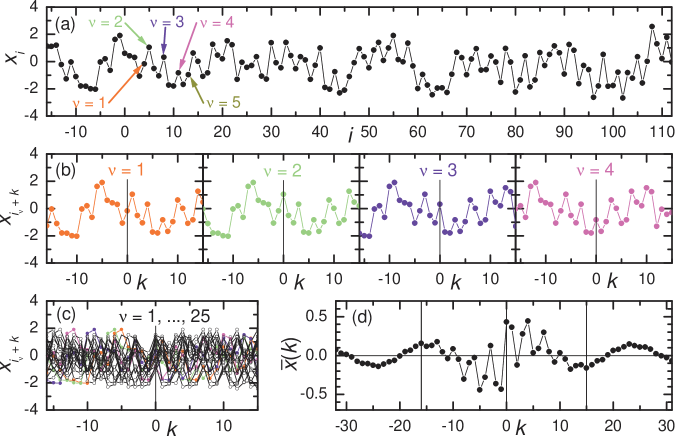
Step 1. Anchor points in the time series are defined according to specific features, e.g., increases (or, alternatively, decreases) in the time series (see Fig. 1(a)). I.e., a point qualifies as an anchor point if
| (1) |
for triggering on increases or decreases, respectively. In order to study a lower frequency regime, averages of successive values of are compared [9]. Typically half of all points of the time series will qualify as anchor points. In general, quasi-periodic oscillations in a noisy time series will result in anchor points predominantly found in the phase of the steepest ascent (or decent for the second alternative in Eq. (1)), i.e., when the phase of the signal itself is close to (or close to ). The phase information of the oscillations is thus obtained from the signal itself, and the signal can be phase-rectified using the anchor points. Note, that in principle any boolean valued function may be used for the definition of anchor points, where true is associated with an anchor while false is not. This allows studying more complex structures in signals.
Step 2. Windows, i.e., surroundings, of length around each anchor point , , are identified (see Fig. 1(b)); is the total number of regarded anchor points. The surrounding of is
| (2) |
The parameter has to be chosen larger than the expected coherence time of the periodicities in the signal; it must definitely exceed the period of the slowest oscillation that one wants to detect. All anchor points with indices smaller than and larger than , i.e., at the very beginning and at the end of the time series, have incomplete surroundings. The same holds for windows containing missing data points due to, e.g., measurement artifacts, instrument failure, or outliers.
Step 3. All windows , are aligned at their anchor points , and the phase-rectified signal average is obtained by averaging over all windows (see Figs. 1(c) and (d)),
| (3) |
If is a missing data point, it is replaced by 0, and is substituted by denoting the number of non-missing points at position . Including windows with missing data points yields better statistics and allows investigation of time series with a few artifacts. In general a well-behaved average can be expected when there are at least to anchor points, i.e., to for the length of the record.
In the average (3), non-periodic components (not phase-synchronized with the anchor points), i.e., non-stationarities, non-identified artifacts, and noise, cancel out. Only events that have a fixed phase relationship with the anchor points, i.e., periodicities and quasi-periodicities, ’survive’ the procedure (see Fig. 1). The PRSA signal represents the most important features of the original data containing all quasi-periodicities aligned with phase zero in the center (at ). Applying the PRSA before traditional spectral analysis significantly improves the quality of the spectra in the presence of noise and non-stationarities [9, 11]. Differences between PRSA curves obtained by applying either of the two criteria in Eq. (1) will indicate missing time reversal symmetry of the original signal. Hence, nonlinear and non time-reversal invariant processes, with different phenomena occurring during increasing and decreasing parts, can be studied in detail. Optionally, it might be meaningful to weight the windows according to some criteria, e.g., according to the magnitude of changes at anchor positions in the trigger signal. With anchors defined at increases Eq. (3) becomes
| (4) |
with weights , e.g., . Of course, other weights could be defined as well.
2.2 Bivariate PRSA (BPRSA)
Now, we suggest a generalization of the univariate PRSA for studying the inter-relations between two signals and . If many signals are recorded simultaneously, representing the dynamics of the complex system, each pair can be characterized accordingly.
The method is nearly identical with the univariate approach described in the previous subsection, except for the usage of different signals in step one ( trigger signal ) and in steps two and three ( target signal ). Specifically, anchor points , are defined for increases (or alternatively decreases) in the trigger signal , i.e. (step 1), while surroundings are defined (step 2) and averaged (step 3) for the target signal , i.e. . This yields the bivariate phase rectified signal average :
| (5) |
The transfer of the anchor points is illustrated in Figs. 2(a),(b).
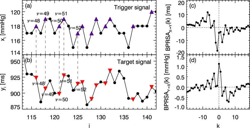
BPRSA is a non-symmetric algorithm, i.e., the exchange of trigger signal and target signal will result in a different BPRSA curve, see 2(c),(d). More complex boolean or weighted anchor criteria, even ones based on more than one trigger signal, are possible. For example, the typical behavior of a target signal can be studied around points of time (anchors) with increases of signal and positive values of signal . For a specific example of a conditional anchor criterion consider the three signals heartbeat intervals, respiratory phase, and blood pressure. One can study characteristic heartbeat intervals (target signal ) around increasing systolic blood pressure (first trigger signal ) and at a certain respiratory phase (second trigger signal ). First attempts revealed promising results for the investigation of baroreflex properties and will be reported in a medical journal.
3 BPRSA and cross-correlation analysis
3.1 Cross-correlation analysis
Although cross-correlation analysis is considered as a well established tool for the study of inter-relations between two signals in many applications, only a few authors have specifically studied its reliability [12, 13, 14]. For two discretely measured signals and , , the normalized cross-correlation function is most commonly defined as
| (6a) | |||||
| (6b) | |||||
Here, and are mean and standard deviation of both series , respectively. This definition assumes that both and do not vary in time, i.e., they do not depend on the segments of the time series selected for the study. This corresponds to the assumption of weak stationarity. Strong stationarity additionally requires constancy of all other moments. For studies discussing the replacement of and by local estimates, e.g. running averages, see [15, 16]. Note, however, that some cross-correlations might be reduced or eliminated by this so-called pre-whitening procedure, which is therefore unsafe.
Another problem of cross-correlation functions is that the exchange of the two signals and corresponds to replacing by , i.e., time inversion. Hence, causality relations between the two series can hardly be assessed. In general, the points of are highly auto-correlated, e.g., is strongly correlated with . I.e., neighboring points in are stronger correlated with each other than neighboring points in the original time series [13, 17]. This self-correlation causes long living trends in , e.g., a slow decay after a peak, which is at risk of misinterpretation.
Furthermore, the sum in Eqs. (6) runs over terms, while it is divided by instead of . This procedure corresponds to a standard averaging procedure only in the limit of very long data (). Nevertheless, most statistical toolkits employ the definition (6), because the convolution theorem and fast Fourier transform can be used to speed up the calculations significantly in this case by application of the Wiener-Khinchin theorem. Some authors even argue for an increase in precision because the normalization reduces the mean-square variance of (see, e.g., [17]). However, this non-matching prefactor results in a bias towards zero with increasing time lag for small , causing a triangular-shaped behavior of . Consequently, the value of for the center of a peak in is systematically underestimated [13]. We are convinced that the correction factor which transforms from Eqs. (6) into the correctly normalized cross-correlation function
| (7) |
must be used to obtain reliable results except for very long data.
If the considered data is not fully stationary, one might want to use only the values with and with for calculating , , , and . This approach is known as local cross-correlation in literature; it is equivalent to the Pearson (product-moment) correlation coefficient for the two overlapping pieces. Since the partial means and standard deviations will depend on , the computational effort is significantly increased. The bias mentioned in the previous paragraph is not completely removed in this approach [13] (although it is weaker than for the standard definitions (6)). In addition, problems with autoregressive moving average processes (ARMA) were reported [17]. Since the cross-correlation approach does not work well for non-stationary data anyway, we do not consider local cross-correlation here.
3.2 Interpretation of BPRSA curves
In BPRSA, anchor points usually occur in all parts of the trigger signal . The average of for all will thus be approximately the global average of the whole signal, i.e., . Consequently, subtraction of this mean from yields positive and negative values as in the cross-correlation function. can thus be interpreted in a similar way as an unnormalized cross-correlation function. If one divides by the global standard deviation, , the resulting quantity
| (8) |
is also normalized. It can be compared with in Eq. (7) and interpreted in a similar way. Note that – different from cross-correlation analysis – this rescaling is just the last step, and does not enter into the calculation of . Hence, the shape of the curve cannot be affected by non-stationarities, i.e., inaccurate . There is no practical advantage of normalized BPRSA, unless the behavior of the curves for different signals, e.g., triggering directions and , shall be directly compared. However, the global mean and global standard deviation might not exist due to non-stationarities and in this case normalization is not recommended.
In some applications it is even preferred to study the unnormalized BPRSA curves. For example, in quantifying the action of blood pressure upon heartbeat regulation via the baroreflex mechanism in the human cardiovascular system, the variation of the time intervals between successive heartbeats in reaction to increases in blood pressure needs to be measured. In this case the units of both signals have to be kept, and the measure characterizing the baroreflex must have the unit ms/mmHg, i.e., time difference divided by pressure difference. In fact, cross-correlation studies can only yield either quantities without units (if normalized) or quantities which are products of both original units. Quantities with the unit of only one original series or their ratio (as needed for the baroreflex) cannot be obtained. Hence, there is no way to obtain a meaningful measure for the baroreflex from a cross-correlation analysis, although the baroreflex is a typical example of a meaningful inter-relation between two components of a complex system.
Effects occurring in for can be easily recognized as consequences of the triggering events in the trigger signal . On the other hand, effects seen in for are likely to be causes for the actual triggering events. Note that a similar conclusion is also valid for the cross-correlation function , since effects observed for and are probably due to interactions from signal onto signal and vice versa. However, BPRSA allows separating these causality effects from nonlinear effects, as we will see in the following.
Altogether, four BPRSA curves can be defined, compared with one cross-correlation function: (triggering on increases in ), (triggering on decreases in ), , and (triggering on ). By comparing these curves, additional information on the linearity of the interactions and time reversal symmetry can be obtained. In the following we will use the symbols and for BPRSA curves obtained by triggering on increases and decreases in the trigger signal only when necessary for distinction. In all other cases means .
If the interaction from signal to signal is linear, we will find , since increases and decreases in must cause opposite effects in . Accordingly, shows that the interaction from to is linear. If the interaction between both signals is fully symmetric, time inversion is equivalent with exchanging the signals, and . Deviations from this behavior show non-symmetric coupling as do deviations from in cross-correlation analysis. However, this can be checked independent of the linear or nonlinear character of the interactions between the signals. Note that normalized BPRSA must be considered in this case, Eq. (8). It is straightforward to write down similar relations for testing further hypothesis regarding the inter-relations between both signals.
3.3 Comparison of cross-correlation analysis and BPRSA
In this subsection we will see how the BPRSA overcomes the disadvantages of cross-correlation analysis described before.
1. Causality and nonlinear interactions. As we have shown in the previous subsection, more information on the linearity or nonlinearity of the interactions and on time-reversal symmetry can be obtained from BPRSA curves than from the cross-correlation function.
2. Time delays. The estimation of (positively or negatively) time-delayed inter-relations between both signals is straightforward, just as in cross-correlation analysis.
3. Missing data and outliers. BPRSA can easily cope with missing data (e.g., measurement artifacts, instrument failure, or outliers) in both series and . Invalid values in just cannot become anchor points. Invalid values in will be disregarded (see text following Eq. (3)).
4. (Non-)stationarity of the data. In the definition of BPRSA (Section 2, in particular Eq. (5)) neither means nor standard deviations of both signals and are needed. Hence, no direct problems arise for non-stationary data. In particular data with a piecewise constant trend, which is often observed in medical data recordings, will cause no problems in BPRSA, because Eq. (5) is a simple linear arithmetic averaging procedure. The deviations from a small or large local average will have the same weight in this averaging procedure. Hence, BPRSA does not need pre-whitening of the data before analysis. Cross-correlation analysis, on the other hand, will be disturbed severely by a piecewise constant trend, because the deviations from the global average will be dominated by this trend (see Subsection 4.3 for an example). The same holds for an oscillating trend in the target signal which is uncorrelated with the trigger signal . However, such a trend in will selectively cause anchor points and thus disturb also BPRSA; consequently more anchor points, i.e., longer data, will be needed!
A slowly varying, monotonous (e.g., polynomial) trend in the target signal will bend the BPRSA curve, since the local means are different in the beginning and at the end of the signal and in the beginning and at the end of each segment. However, this bending is definitely not stronger than a similar bending of the cross-correlation function. Trends in the trigger signal will modify the fraction of anchor points for increases and decreases, which has little effect on unless these trends are very strong.
5. Enhanced auto-correlations. Unlike the cross-correlation function [13, 17], which is often dominated by low frequencies, BPRSA does not show artificially enhanced auto-correlations. On the contrary, low frequencies are reduced due to the filtering characteristics (see next point). This makes BPRSA particularly attractive for studying signals with underlying - rather than white noise. Note that -noise is prevalent, e.g., in medical and geophysical data.
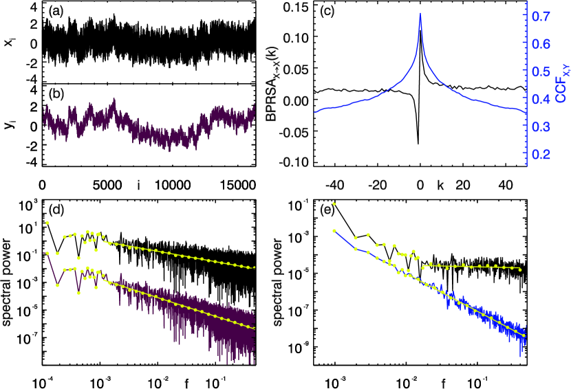
6. Filtering characteristics. Figure 3 compares the spectral properties of both, cross-correlation analysis and BPRSA. Since many interesting data contain long-term auto-correlations and are characterized by -noise in their power spectra, with around 1, we start with two such noise series (see Fig. 3(a,b)) with and (see Fig. 3(d)). The power spectrum of the cross-correlation function decays as (see Fig. 3(e)). It is thus dominated by low-frequency components. The BPRSA curve, on the other hand, yields a nearly flat power spectrum (see also Fig. 3(e)). Therefore, additional peaks and quasi-periodicities can be noticed and determined much easier.
The filtering characteristics of BPRSA can be motivated as follows. The scaling behavior of the BPRSA spectrum is influenced by the anchoring procedure in the trigger signal and by the averaging of the target signal. We want to estimate the probability that an oscillating component with frequency , in the target signal affects under the condition that an oscillation with the same frequency , causes anchor points in the trigger signal . Firstly, has to cause anchor points at positions , meaning has to be larger than for anchor criterion Eq. (1a). This is a valid approximation except for very high frequencies . The deviation becomes maximal for with any integer . Since anchor points are primarily generated at or close to phase zero of the considered component , the later averaging is phase-rectifying in terms of the trigger signal. The value of the maxima is and thus the probability to anchor is proportional to . On the other hand, the component has an effect proportional to its amplitude due to the averaging procedure of Eq. (3) and therefore . The amplitude of the considered spectral components in is thus determined by . If we consider two signals and consisting of correlated noise with power spectra
| (9) |
we obtain
| (10) |
with , yielding if both and are close to one or their average is close to one.
4 Three illustrative examples
Since BPRSA has significant advantages over cross-correlation analysis for studying data with noise and/or nonlinear interaction as well as non-stationary data, one can imagine several applications. Here, we describe three specific situations and illustrate the performance of BPRSA on model data.
4.1 White noises with linear relation
We consider two independent white noise signals and with zero mean and unit variance. Based on we generate the signal by introducing a linear unidirectional coupling with in a certain frequency band. This is generated by calculating the linear combination of and one or more bandpass filtered components of ,
| (11) |
The bandpass filtering is done in Fourier space, and denotes the -th element of the series obtained from the related -th bandpass filter operator acting on . The prefactors include the coupling strengths and directions . Finally, is normalized to obtain zero mean and unit variance. Fig. 4(a) illustrates the original noise , while Figs. 4(b,c) show and for two different values of and .
Different coupling strengths are reflected by different amplitudes of and , while a different coupling direction results in a different sign of (compare Figs. 4(d,e)). Since we consider linear coupling, as discussed in Section 3.2 and illustrated in Figs. 4(d,e). There is no advantage over which looks very similar in this example.
4.2 Nonlinear relation
The response of the BPRSA to nonlinearly coupled trigger and target signals strongly depends on the type of the coupling. The most simple nonlinear coupling is the absolute value. Let us assume a sinusoidal trigger signal without noise and a target signal that only contains the absolute value of , yielding a frequency doubling. When calculating the BPRSA all oscillations cancel out and . In the presence of additional -noise the BPRSA will basically show features of the noise and possibly finite size effects. The same holds for similar nonlinear coupling, e.g., raising to an even power. On the other hand, this elimination of higher harmonics might be an advantage if one wants to clarify a complex relationship between two unknown signals.
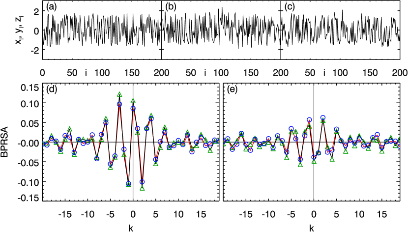
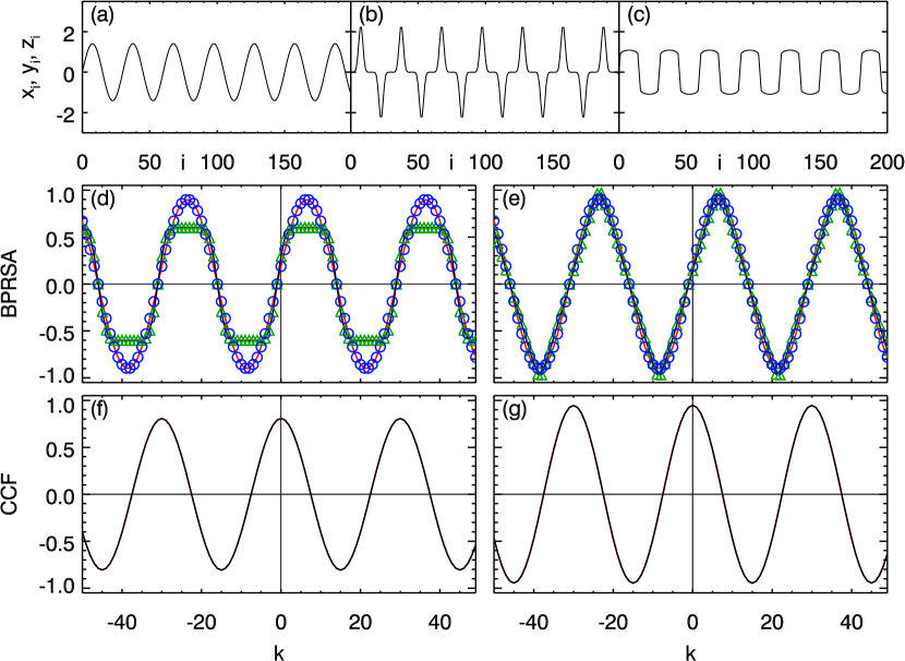
Now, we study nonlinear coupling without frequency doubling. Three simple oscillating series are defined by
| (12) |
and illustrated in Figs. 5(a-c). The large power of has been chosen for visual reasons only; it enhances the differences as does the absence of noise. The cross-correlation analysis (see Figs. 5(f,g)) cannot distinguish (i) the cases and as well as (ii) both possible analysis directions. Studying only the cross-correlation function could thus lead to the false conclusion of equivalently related signals and . BPRSA, on the other hand, can clearly distinguish the four cases except for . However, one has to keep in mind that the shape of the BPRSA curve needs not be the same as the original target signal (compare Figs. 5(b,d)). A presence of noise might disturb the BPRSA signal, making the identification of characteristics in trigger and target signal more difficult, depending on the signal to noise ratio.
4.3 Influence of Trends in the signal
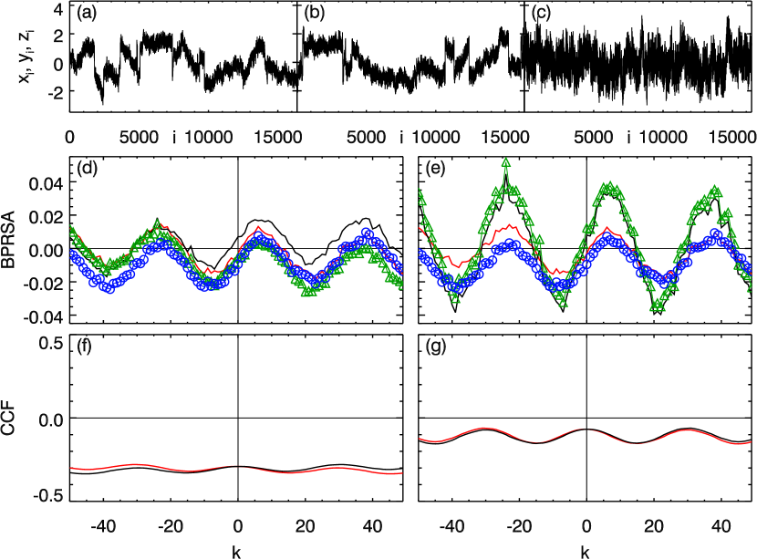
Now let and be two independent -noise signals with zero mean and unit variance generated by Fourier filtering. Furthermore, we add to both signals a periodic component . Moreover, non-stationarities are introduced by adding piecewise linear trends as follows. We start with some initial value for the slope and the initial offset . At random positions, the offset and the slope are changed randomly within a previously defined range; the trends added to and are independent (see Figs. 6(a,b)). For comparison we define a third signal that equals without trends (Fig. 6(c)).
Trends in the trigger signal will hardly affect the identification of the anchor points, because the anchor criteria defined in Eq. (1) is only based on local fluctuations. Note, that this might be different when using a more sophisticated boolean anchor function as discussed earlier (compare BPRSA directions and in Fig. 6(d,e)).
On the other hand, the influence of trends in the target signal cannot be neglected (see Fig. 6(e)). In case of a significant global trend in the target signal, e.g., more decreasing parts than increasing parts, the global trend will be present in the BPRSA curve, although it is diminished. Note, that due to trends which do not cancel out completely in general (compare solid lines and triangles in Figs. 6(d,e)). When the BPRSA shows no trend at all, the target signal is either characterized by no trends or the duration and slopes of increasing and decreasing trends cancel out.
As an implication of the different influences of trends in the trigger and target signal one can identify which signal is disturbed by trends by comparing the BPRSA for opposite trigger-target directions (). This is inherently impossible with cross-correlation analysis since the algorithm does not distinguish between both signals. Besides, trends are harmful for the definition of a global mean and thus disturb the standard cross-correlation analysis. Therefore, its results may suggest a wrong correlation behavior. In Figs. 6(f),(g) one finds, by chance, anti-correlated behavior although the signals themselves, i.e., the sinusoids, are strongly positively correlated. For the same reason a normalized BPRSA as defined in Eq. (8) cannot be applied here. Of course, in this simple example the use of the local cross-correlation function, which is based on local means rather than on a global mean, might help to remove the influence of the trends.
5 Summary and Outlook
In summary we have shown that the BPRSA method has several advantages compared with conventional cross-correlation analysis in the detection of quasi-periodicities in noisy non-stationary data with oscillations of finite coherence time. The method allows the analysis of the inter-relationship between two signals, in particular effects in one signal triggered by events in another signal.
This capability can be useful for the study of the inter-relation between respiration, heart rate and blood pressure, i.e., the cardiovascular regulation, which is an important topic in human physiology. Cardiovascular functions are controlled by the tone of the sympathetic and parasympathetic (autonomic) nervous system that is influenced by the baroreflex, a homeostatic regulation that maintains a ’stable’ blood pressure. An elevated blood pressure reflexively causes the blood pressure to decrease and vice versa. It is controlled through several stretch sensitive mechanoreceptors (baroreceptors)111Activation of the baroreceptor results in an inhibition of sympathetic components and activation of parasympathetic or vagal components. Due to an initially elevated blood pressure activated baroreceptors tend to decrease cardiac output via a decrease in contractility resulting in a lower heart rate and finally in a decrease in blood pressure. A low blood pressure level relaxes the mechanoreceptor and stops the sympathetic inhibition and results in an increased contractility, heart rate and blood pressure.. It is believed that cardiovascular illnesses disturb the baroreflex. Related parameters might thus improve currently used predictors. Hence, the detection of quasi-periodicities reflecting regulation processes of the autonomic cardiac nervous system coinciding with increases or decreases of blood pressure in long records of human heart rate is of high clinical relevance. Autonomic dysfunction is closely related to cardiac mortality and susceptibility to life-threatening arrhythmic events [18]. The assessment of heart rate variability by the PRSA based deceleration capacity (DC) parameter [10, 11] was shown to be superior to spectral parameters proposed earlier for risk prediction [19]. BPRSA seems to be promising for the definition of an advanced risk predictor that respects the coupling of heart rate variability and blood pressure.
Further possible applications of BPRSA in biology and physiology include rhythmic motions of limbs in walking, muscle contractions, rhythms underlying the release of hormones that regulate growth and metabolism, periodicities in gene expression, membrane potential oscillations, oscillations in neuronal signals, and circadian rhythms [1, 2]. We believe that the range of suitable applications for the BPRSA method also includes quasi-periodic geophysical data, e.g., the El-Niño phenomenon, sunspot numbers, and ice age periods [3]. In addition, the analysis of complex elastic wave patterns to study seismic events or to determine material properties of granular matter might be improved by BPRSA. The study of non-stationary quasi-periodic complex waveforms is also a common task in the analysis and recognition of speech or music.
Acknowledgement: This study was supported by grants from the Deutsche Forschungsgemeinschaft (grant KA 1676/3) and the European Union (project DAPHNet, grant 018474-2).
References
- [1] J. Tyson, in: Computational Cell Biology: An Introductory Text on Computer Modeling in Molecular and Cell Biology, J. Tyson, J. Wagner, E. Marland, C. Fall (Eds.), Springer, New York, 2002.
- [2] L. Glass, Nature 410 (2001) 277.
- [3] H. von Storch, F. Zwiers, Statistical Analysis in Climate Research, Cambridge University Press, 2001.
- [4] M.B. Priestly, Nonlinear and Non-Stationary Time Series, Academic Press, New York, 1988.
- [5] P.J. Brockwell, R.A. Davis, Introduction to Time Series and Forecasting, Springer, Berlin, 2003.
- [6] G.E.P. Box, G.M. Jenkins, G.C. Reinsel, Time Series Analysis, Forecasting and Control, Prentice-Hall, Englewood Cliffs, 1994.
- [7] H. Kantz, T. Schreiber, Nonlinear Time Series Analysis, Cambridge University Press, 2004.
- [8] C.K. Peng, S.V. Buldyrev, S. Havlin, M. Simons, H.E. Stanley, A.L. Goldberger, Phys. Rev. E 49 (1994) 1685.
- [9] A. Bauer, J.W. Kantelhardt, A. Bunde, P. Barthel, R. Schneider, M. Malik, G. Schmidt, Physica A 364 (2006) 423.
- [10] A. Bauer, J.W. Kantelhardt, P. Barthel, R. Schneider, T.Mäkikallio, K. Ulm, K. Hnatkova, A. Schömig, H. Huikuri, A. Bunde, M. Malik, G. Schmidt, Lancet 367 (2006) 1674.
- [11] J.W. Kantelhardt, A. Bauer, A.Y. Schumann, P. Barthel, R. Schneider, M. Malik, G. Schmidt, Chaos 17 (2007) 015112.
- [12] B.M. Peterson, I. Wanders, K. Horne, S. Collier, T. Alexander, S. Kaspi, D. Maoz, PASP 110 (1998) 660.
- [13] W. Welsh, PASP 111 (1999) 1347.
- [14] R. Vio, W. Wamsteker, PASP 113 (2001) 86.
- [15] J.D. Scargle, Astrophys. J. 343 (1989) 874.
- [16] W.H. Press, G.B. Rybicki, J.N. Hewitt, Astrophys. J. 385 (1992) 404.
- [17] G.M. Jenkins, D.G. Watts, Spectral Analysis and Its Applications, 1st Edition, San Francisco: Holden-Day, 1969.
- [18] B. Lown, R.L. Verrier, New Engl. J. Med. 294 (1976) 1165.
- [19] J. Bigger, J. Fleiss, R. Steinman, L. Rolnitzky, R. Kleiger, J. Rottman, Circulation 85 (1992) 164.