Precise radial velocities of Polaris: Detection of Amplitude Growth

Abstract

We present a first results from a long-term program of a radial velocity study of Cepheid Polaris (F7 Ib) aimed to find amplitude and period of pulsations and nature of secondary periodicities. 264 new precise radial velocity measurements were obtained during 2004–2007 with the fiber-fed echelle spectrograph Bohyunsan Observatory Echelle Spectrograph (BOES) of 1.8m telescope at Bohyunsan Optical Astronomy Observatory (BOAO) in Korea. We find a pulsational radial velocity amplitude and period of Polaris for three seasons of 2005.183, 2006.360, and 2007.349 as 2K = 2.210 $\pm$ 0.048 km s^-1, 2K = 2.080 $\pm$ 0.042 km s^-1, and 2K = 2.406 $\pm$ 0.018 km s^-1 respectively, indicating that the pulsational amplitudes of Polaris that had decayed during the last century is now increasing rapidly. The pulsational period was found to be increasing too. This is the first detection of a historical turnaround of pulsational amplitude change in Cepheids. We clearly find the presence of additional radial velocity variations on a time scale of about 119 days and an amplitude of about $\pm$ 138 m s^-1, that is quasi-periodic rather than strictly periodic. We do not confirm the presence in our data the variation on a time scale 34–45 days found in earlier radial velocity data obtained in 80’s and 90’s. We assume that both the 119 day quasi-periodic, noncoherent variations found in our data as well as 34–45 day variations found before can be caused by the 119 day rotation periods of Polaris and by surface inhomogeneities such as single or multiple spot configuration varying with the time.

1 Introduction

Polaris ($\alpha$ UMi, HIP 11767, HD 8890, HR 724 ) is one of the most famous Cepheid variable stars. In addition to its special location on the celestial sphere, Polaris has many interesting astrophysical features. It is a member of a triple system. It is the brightest and the closest Cepheid variable with very low pulsational amplitude. It has been extensively studied over 1.5 centuries for the pulsational amplitude and period changes using photometric and spectroscopic observations. Perhaps the most remarkable feature of Polaris as a Cepheid variable is that the period and amplitude of pulsation is changing very rapidly. The pulsation period is rapidly increasing with the rate of about 4.5 s y^-1 (Turner et al. 2005 and references herein). More interesting is the change of amplitude. It is discovered that the pulsational amplitude has been decreasing dramatically during the 20th century (Arellano Ferro 1983; Dinshaw et al. 1989). So it was predicted that the pulsation of Polaris would completely stop by the end of the 20th century. However, Kamper & Fernie (1998) notes that decline of radial velocity (RV) amplitude has stopped abruptly. Figure 5 of Hatzes & Cochran (2000) shows the increase of amplitude, but they did not state that explicitly. Some recent photometric observations also indicate the same trend in the amplitude (Davis et al. 2002; Engle et al. 2004).

2 Observations and data reduction

The new RV observations of Polaris were carried out during November 2004 to June 2007 using the fiber-fed high resolution (R=90,000) echelle spectrograph BOES (Kim et al. 2007) attached to the 1.8m telescope at BOAO. Using a 2k x 4k CCD, the wavelength coverage of BOES is 3600–10,500 Å with $\sim$ 80 spectral orders in one exposure. Observations were acquired through iodine absorption cell (I${}_{2})$ to provide the precise RV measurements. Total of N=264 spectra were recorded; the exposure time varied from 60 to 300 s depending on the sky condition to get a typical S/N ratio of 250. The extraction of normalized 1–D spectra was carried out using IRAF (Tody 1986) software package. After extracting normalized 1–D spectra, the RV measurements were undertaken using a code called RVI2CELL (Han et al. 2007) which was developed at BOAO. RVI2CELL adopted basically the same algorithm and procedures described by Butler et al. (1996). However we model the instrument profile using the matrix formula descried by Endl et al. (2000). We solved the matrix equation using singular value decomposition instead of maximum entropy method adopted by Endl et al. (2000). With these configuration, we achieved the typical internal RV accuracy between 10 and 15 m s^-1 depending on the quality of spectra.

3 Results

Figure 1 plots the relative RV measurements for 2004–2007 season of observations. The solid line is a zero-point adjusted trend for binary orbit calculated according to the period of 29.59 years and orbital elements given by Wielen et al. (2000). To study pulsations, we first removed the RV variation due to orbital motion. Next, we applied the Discrete Fourier Transform (DFT) analysis for unequally spaced data to all de-trended 2004–2007 RV data. We used for analysis the computer code PERIOD04 (Lenz & Breger 2005). The top panel in Figure 2 shows the resulting DFT periodogram of all data. We easily found a main frequency of $f{{}_{1}}$ = 0.251757 $\pm$ 0.000008 c d^-1 ($P{{}_{1}}$ = 3.97208 $\pm$ 0.00013 days). The whole 2004–2007 data phase diagram of Polaris phased with this period is plotted in Figure 3. There are visible scatters, and two order values (near JD 2453902) exceed the accuracy of our individual RV measurements ($\sim$ 10 m s^-1). This scatter seems to be due to additional intrinsic RV variations to the dominant pulsation mode, already known for Polaris (Dinshaw et al. 1989; Kamper 1996; Kamper & Fernie 1998; Hatzes & Cochran 2000). We removed the best fit sine-wave signal from dominant period from all the data string. The DFT analysis of RV residuals is shown in second from top panel in Figure 2. The highest peak at $f_{2}^{{}^{\prime}}$ = 0.00799 $\pm$ 0.00010 c d^-1 ($P{{}_{2}}^{{}^{\prime}}$ = 125.1 $\pm$ 0.1 days) has an amplitude of 2K = 0.38 $\pm$ 0.02 km s^-1.

One might suspect that the secondary signal at $f^{\prime}_{2}$ found in our 2004–2007 data residuals is due to removing dominant pulsations with fixed amplitude and period which are actually varying during this time interval. Here our main concern is to estimate the amplitude and period of the dominant pulsations for short subsets as accurately as possible and remove it from RV variations in order to study possible residual signals. In determining the period and amplitude variation, the data were divided into three subsets: Set 1, Set 2, and Set 3. These subsets are marked in Figure 1. The RV data characteristics are given in second, third, and forth columns of Table 1. Then, for each data set, we tried to find best fit frequency and amplitude for a dominant pulsation. Figure 4 shows a dominant period fit to every subset of the data. The r.m.s. residuals after the sinusoidal fitting of Set 1, Set 2, and Set 3 are 111 m s^-1, 149 m s^-1, and 63 m s^-1 respectively, much larger than the typical error of RV data, 10–15 m s^-1. It is, indeed, because there exists unmodelled RV variation in addition to the sinusoidal signal. Table 1 shows the result of the period analysis: periods and amplitudes of pulsations found for all three sets. We applied the same period analysis to the most recent RV data published for Polaris. The period and amplitude found during our re-analysis are also given in Table 1.

To study additional variability, the residuals after removing the best fit dominant period and amplitude from each set were combined, resulting in data string shown in Figure 5. As seen by eye, there is still very strong $\sim\pm$ 350 m s^-1 and about 120 days time scale variability. The shape of RV variability has the steep rise of RV from negative to positive values and rapid drop back to negative values. Such type of variability resemble closely the RVs variations due to a contrast surface spot passing across the visible disk in some types (e.g. Ap) of stars. To get the accurate period the DFT analysis was applied to the residual data. The DFT amplitude spectrum is shown in the third panel from the top panel in Figure 2. The largest 138 $\pm$ 8 m s^-1 peak is at $f_{2}$ = 0.00840 $\pm$ 0.00003 c d^-1 (P₂ = 119.1 days). The residual data phased to this period shown in Figure 6. The DFT of residuals after removing of the secondary periodicity is shown in the bottom panel in Figure 2; it does not show any significant peaks.

The check whether secondary periodicity may be due to unrecognized aliasing problem and unfavorable time sampling of RV data (note, that the strongest sidelobes of the spectral spectral window function are 1 c d^-1 equally spaced) we modeled the dominant mode pulsations by mono-periodic sinusoidal signal having the same time sampling as the original Polaris RV data. Note, that DFT of this mono-periodic signal is actually the spectral window function centered at $f_{1}$. We added to this mono-periodic signal the normally distributed noise with amplitude of 138 m s^-1. The DFT analysis of these artificial data is shown in right panels (top and bottom) in Figure 6. As can be seen from the bottom panel, after removal of the artificial signal, the amplitude spectrum do not show any significant signal at 0.008 c d^-1, confirming that secondary 119-day periodicity we found is not an artifact.

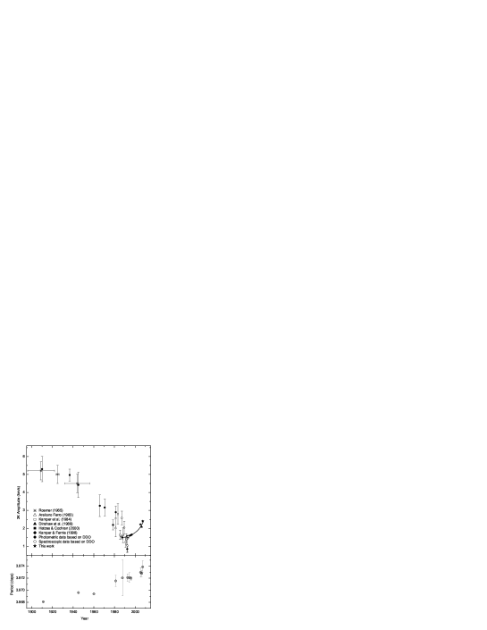
Figure 7: Variations of the pulsational RV amplitude and period of Polaris during the last century. (Top) Filled and open circles denote the result from DDO photometric and spectroscopic measurements, respectively. To convert photometric determination to RV determination, conversion factor of $\sim$ 50 (Kamper $\&$ Fernie [1998] and Fernie et al. [1993]) was used. The solid line is a polynomial fit to the recent RV measurements. Error bars of Hatzes $\&$ Cochran (2000), Kamper $\&$ Fernie (1998), and this work are smaller than the symbols. (Bottom) The period variations; for the first three points, there are no reference in error bars.

Figure 7 shows a century-long variations of the pulsational amplitude and period of Polaris. As seen, our new data obtained for three subsets of our 2004–2007 observations reveals that after a decade of standstill the amplitude of pulsation is now rapidly increasing. We can claim now safely that the era of amplitude decrease of Polaris was finished in the end of 1980’s and replaced with a new, quickly uprising amplitude trend in the beginning of the 1990’s.

4 Discussions

Historic change of the sign of amplitude variations in Polaris, that we securely detected, doesn’t yet have an analogy among other Cepheids. Polaris is crossing the instability strip for the first time and lies well in its center for fundamental mode pulsators or well inside and near the hot bounds of instability strip for a first overtone pulsators (Turner et al. 2005). We can suggest that switching of amplitude change from decay to growth found in our observation is not a direct result of evolution to a red border and the decrease of the efficiency of the excitation mechanism, but might be relevant to the unrecognized effect of mode interaction. We confirm the increase of pulsational period too.

The detected long-term characteristic period of 119 days is much longer compared to the 9.75 days period by Kamper et al. (1984), 45.3 days by Dinshaw et al. (1989), 34.3 days by Kamper & Fernie (1998) or 40.2 days by Hatzes & Cochran (2000) reported in the 80’s and 90’s data. We do not confirm the existence of any of the aforementioned periods in our data. Dinshaw et al. (1989) argue that approximately 45-day period, that is not coherent, arises from one or more surface features on Polaris carried across the disk by rotation. Hatzes & Cochran (2000) have found very reliable bisector variations with the same period as in RVs and re-discussed three mechanisms of the low amplitude residual RV variations in Polaris: a low-mass companion, long-periodic nonradial stellar pulsations, or rotational modulation by surface features. They modeled the residual RV and bisector variations for all hypotheses - namely, existence of a surface microturbulence, cool or hot spots and 45 day rotation period, or the l=4, m=4 nonradial mode pulsations and found reliable RV amplitude fit for all of them. However, the bisector span velocity for all hypotheses had a unmodelled phase shifts, indicating that all of these models do not satisfy completely observations. Hatzes & Cochran (2000) concluded, that among considered hypotheses the nonradial pulsations has better agreement with modelling.

In our work based on long-term high-precision RVs, we do not confirm any of the secondary period found earlier, but find clear 119.1 day characteristic time of variations. This is a longest period of intrinsic variations of Polaris found so far.

Summarizing all previous investigation, we can claim that the secondary variations seen in Polaris are not coherent on a long time-scales so we can firmly reject first two hypotheses involving the companion and coherent non-radial pulsations. Note, that period 119 days is too long compared to a period of fundamental mode pulsations of Polaris and cannot belong to normal acoustic modes.

We suggest two possible explanations of secondary radial velocity variations:

a) The diversity in secondary periods found in Polaris is likely the result from the rotational modulation of RVs by a single or multiple surface spots and assume that the rotation period is about 119 days. In the case of multiple spots, the observed periods about 40 days or about 34 days are close to fractions of 119 day period. The rotational velocity of Polaris is $vsini$ = 8.4 km s^-1 (Hatzes & Cochran, 2000). The radius of Polaris 33 $\pm$ 2 $R_{\odot}$ was found by Turner et al. (2005) from the distance to Polaris 94 $\pm$ 4 pc and the angular diameter 3.28 $\pm$ 0.02 mas given by Nordgren et al.(2000). With these parameters and assumed rotation period of 119 days, the equatorial rotation velocity is $v_{\rm eq}$ = 14 km s^-1, that yields the inclination angle of rotation axis $i$ = $38^{\circ}$. The projected rotational and expected equatorial velocities of Polaris are in a quit good agreement with the determined mean projected rotational velocities $\overline{vsini}$ = 15.8 $\pm$ 1.4 km s^-1 of a sample of eleven F6-F7 Ib supergiants selected from the Ib supergiant list of De Medeiros et al. (2002).

b) We cannot exclude also that long-term cyclic variations of radial velocities of Polaris is a results of oscillatory variations of the mean radius of Polaris stochastically driven with yet unrecognized physical mechanism. Not excluded, that such a long-term, non-coherent and small radius variations are intrinsic to many F type supergiant stars and Cepheids, but in classical Cepheids are hidden in a large amplitude of of the dominant mode pulsations and were not detected due to limited RV accuracy and sparse time sampling of RV curves in previous RV investigations. If true, Polaris might be a first Cepheid star with well documented observational detection of such of modulation. The another good example might be a F5 Ib supergiant $\alpha$  Per that show long-term (see Fig. 1 in Hatzes and Cochran 1995) variations. The detailed comparative precise RV study of a sample of F-type supergiant stars including Cepheids can provide additional constrains on the nature of long-term radius variations detected in Polaris.

The check of spot hypothesis and detailed analysis of line profile and surface temperature variations in Polaris based BOES observations is out-of the scope of the current work which is devoted to the study of pulsational amplitude of RVs and will be presented in our next paper.

5 Conclusions

First results of our long-term monitoring of Polaris show remarkable changes in the amplitude and the period of pulsations that occurred at the end of 20th and the beginning of 21st century. The half-century-long pulsational amplitude decay was replaced with the rapid amplitude growth while the growth of pulsational period continues. We also detected the 119-day secondary RV variation that is about three times longer that secondary periodicities reported before. We concluded that 119 day variations are not coherent on long time scales and discussed possible nature of these variations.

Figure 1: RV measurements of Polaris during 2004–2007. Solid line shows the decline of orbital RVs within interval of observations.

Figure 2: The amplitude spectra of DFT analysis for the entire RV measurements for Polaris. Left panel: (Top) DFT of original data. Largest peak is at $\it f_{1}$ = 0.251757 c d^-1. (Second) DFT of RV residuals after removing contribution from $\it f_{1}$. The second peak is at $f{{}_{2}}^{{}^{\prime}}$ = 0.00799 c d^-1. (Third) DFT of merged residual RV after removing of the best fit $\it f_{1}$ contribution from individual subsets (Set 1, Set 2, and Set 3). The secondary peak is at $f{{}_{2}}$ = 0.00840 c d^-1. (Bottom) DFT of residuals after removing of $f{{}_{1}}$ and $f{{}_{2}}$. Right panel: (Top) The amplitude spectrum of artificial sin-wave signal having the same frequency, amplitude and data point sampling as the dominant $f_{1}$ mode but co-added with normally distributed noise of the amplitude of 138 m/s. (Bottom) DFT of residual RV after removing contribution from $f_{1}$.

Figure 3: Entire RVs of Polaris de-trended for orbital variations. Solid line is a dominant period fit to every subsets of the data.

Figure 4: Phase curve of original data phased to the best fit period $P_{1}$ = 3.97208 days.

Figure 5: Merged residual RVs after removing the best fit amplitude and period solutions to data from three subsets.

Figure 6: Residual RV phased with a best fit period of $P_{2}$ = 119.1 day from three subsets.

Table 1: The period and amplitude of Polaris. $\sigma$ is r.m.s. residuals after main signal fitting

Data	mean epoch	N	$\sigma$	Semi-amplitude	Dominant Period	Period in residuals
	(duration)		(km s-1)	(km s-1)	(days)	(days)
Dinshaw	1987.674 (0.660)	174	0.661	0.742 $\pm$ 0.068	3.97206 $\pm$ 0.00307	45
Hatzes	1992.693 (1.698)	40	0.140	0.755 $\pm$ 0.032	3.97212 $\pm$ 0.00056	17, 40
Kamper1	1994.492 (0.414)	71	0.098	0.786 $\pm$ 0.017	3.97208 $\pm$ 0.00081	34
Kamper2	1995.973 (1.249)	129	1.107	0.825 $\pm$ 0.013	3.97200 $\pm$ 0.00029
set 1	2005.183 (0.575)	34	0.111	1.105 $\pm$ 0.024	3.97300 $\pm$ 0.00080	$\backslash$
set 2	2006.360 (0.870)	117	0.149	1.040 $\pm$ 0.021	3.97284 $\pm$ 0.00047	$\rangle$ 119
set 3	2007.349 (0.168)	113	0.063	1.203 $\pm$ 0.009	3.97394 $\pm$ 0.00098	$/$

References

- Arellano Ferro (1983) Arellano Ferro, A. 1983, ApJ, 274, 755
- Butler et al. (1996) Butler, R. P., Marcy, G. W., Williams, E., McCarthy, C., Dosanjh, P., & Vogt, S. S. 1996, PASP, 108, 500
- Davis et al. (1975) Davis, J. J., Tracey, J. C., Engle, S. G., & Guinan, E. F. 2002, BAAS, 34, 1296
- De Medeiros et al. (2002) De Medeiros, J. R., Udry, S. Burki, G. & Mayor, M. 2002,A&A, 395, 97
- Dinshaw et al. (1989) Dinshaw, N., Matthews, J. M., Walker, G. A. H., & Hill, G.M. 1989, AJ, 98, 2249
- Endl et al. (2000) Endl, M., Kürster, M., & Els, S. 2000, A&A, 362, 585
- Engle et al. (2004) Engle, S. C., Guinan, E. F., & Koch, R. H. 2004, BAAS, 36, 744
- Fernie et al. (1993) Fernie, J. D., Kamper, K. W., & Seager, S. 1993, ApJ, 416, 820
- (9) Han, I., Kim, K.-M., & Lee B.-C. 2007, PKAS, 22, 75
- Hatzes & Cochran (1995) Hatzes, A. P., & Cochran, W. D. 1995, ApJ, 452, 401
- Hatzes & Cochran (2000) Hatzes, A. P., & Cochran, W. D. 2000, AJ, 120, 979
- Kamper et al. (1984) Kamper, K. W., Evans, N. R., & Lyons, R. W. 1984, JRASC, 78, 173
- Kamper (1996) Kamper, K. W. 1996, JRASC, 90, 140
- Kamper & Fernie (1998) Kamper, K. W., & Fernie, J. D. 1998, AJ, 116, 936
- Kim et al. (2007) Kim, K. M., Han, I., Valyavin, G. G., Plachinda, S., Jang, J. G., Jang, B.-H., Seong, H. C., Lee, B.-C., Kang, D.-I., Park, B.-G, Yoon, T. S., Vogt, S. S., 2007, PASP, 119, 1052
- Lenz (2005) Lenz, P., Breger M. 2005, Commun. Asteroseismology, 146, 53
- Nordgren (2000) Nordgren, T. E., Armstrong, J. T., German, M.E., Hindsley R. B., Hajian, A. R., Sudol, J. J. & Hummel, C. A. 2000, ApJ, 543, 972
- Roemer (1965) Roemer, E. 1965, ApJ, 141, 1415
- Tody (1986) Tody, D. 1986, Proc. SPIE, 627, 733
- Turner et al. (2005) Turner, D. G., Savoy, J., Derrah, J., Abdel-Sabour Abdel-Latif, M., & Berdnikov, L.N. 2005, PASP, 117, 207
- Wielen et al. (2000) Wielen, R., Jahreiß, H., Dettbarn, C., Lenhardt, H., & Schwan, H. 2000, A&A, 360, 399