Folding and unfolding kinetics of a single semiflexible polymer

Abstract

We theoretically investigate the kinetics of the folding transition of a single semiflexible polymer. In the folding transition, the growth rate decrease with an increase in the number of monomers in a collapsed domain, suggesting that the main contribution to dissipation is from the motion of the domain. In the unfolding transition, dynamic scaling exponents, $1/8$ and $1/4$, were determined for disentanglement and relaxation steps, respectively. We performed Langevin dynamics simulations to test our theory. It is found that our theory is in good agreement with simulations. We also propose the kinetics of the transitions in the presence of the hydrodynamic interaction.

I Introduction

Compared to our understanding of the equilibrium states of polymers, our understanding of far from equilibrium is quite primitive. Recently, the kinetic properties of single polymer molecules have become experimentally tractable, and they have been investigated mainly because of their biological importance. Although the kinetics of ordering are well understood and several investigations have been carried out on flexible polymers, the kinetics of semiflexible polymers are not as well understood.

Most biopolymers, including DNA and many proteins, have bending rigidity; therefore, they are classified as semiflexible polymers. It is expected that bending rigidity plays an important role in the structural stability and function of these biomacromolecules. Recent experiments and simulations have clarified that a single semiflexible polymer exhibits first-order phase transition between an swollen coil state and a folded compact state as the solvent quality decreases Takahashi et al. (1997). A single semiflexible polymer folds into various kinds of ordered structures depending on its bending rigidity and temperature, such as a toroid or a cylinder Noguchi et al. (1996).

The folding kinetics of a flexible polymer was first discussed by de Gennes with the scaling theory de Gennes (1985); Buguin et al. (1996), and then various methods have been proposed, such as Uniform Expansion Method Pitard and Orland (1998); Pitard (1999) and Gaussian Self-consistent method Timoshenko et al. (1995), where the latter was extended to the folding kinetics of a semiflexible polymer Kuznetsov et al. (1996). Numerical simulations such as the Brownian Dynamics Byrne et al. (1995); Chang and Yethiraj (2001) and Monte Carlo Ostrovsky and Bar-Yam (1995); Crooks et al. (1999) simulations have been carried out. Most of the simulations ignored the hydrodynamic interaction. Recently, the authors in Kikuchi et al. (2002, 2005) have developed a new algorithm, which enables us to elucidate the features of the hydrodynamic interaction in the kinetics of the collapse transition of a flexible polymer. These investigations have revealed that a flexible polymer forms a pearl-necklace conformation at an early stage of a transition and reaches the globule state via the growth of each pearl Klushin (1998); Halperin and Goldbart (2000). Although the globule is compact, it does not reach the most stable state. Therefore, at a later stage of the transition, segments realign so as to form the equilibrium conformation Grosberg et al. (1988). The experiments with poly($N$-isoporpylacrylamide) (PNIPAM) were found to be consistent with the theoretical and numerical results Xu et al. (2006).

In this article, we discuss the transition kinetics in single semiflexible polymers. Our picture is that the folding transition consists of the nucleation and growth steps, and the unfolding transition has three different regimes: swelling, disentanglement, and relaxation Yoshinaga (2006). Nucleation and growth processes have been observed in the simulations of single semiflexible polymers and experiments on single DNA molecules. On the other hand, to our knowledge, the mechanism of the unfolding transition has been much less elucidated, since it is difficult to observe the microscopic dynamics of chain segments. In Rabin et al. (1995); Lee et al. (2004), authors theoretically and computationnally proposed the existence of a topological constraint in single flexible polymers in the unfolding transition. Our purpose is to study the time evolution of a macroscopic variable such as the long-axis length, which is experimentally observable. We derive equation of motions for the variables and determine the dynamic scaling exponents in the unfolding transition on the basis of a scaling analysis. It is of importance to note that the validity of our picture can be verified by comparison with exponents in experiments and simulations.

The reminder of this paper is organized as follows: In section II, we present an overview of our method. The results of the theoretical analysis of the folding and unfolding transitions are shown in section III and IV, respectively. Then, in section V, we demonstrate the results of simulations and compare them with our theoretical results. We discuss the hydrodynamic interaction in section VI. Section VII is devoted to the justification of our theory with investigation of kinetic pathways. In section VIII, we summarize our results.

II Theory

In general, it is not trivial to write down the equations of motion of course-grained variables such as a gyration radius. In de Gennes (1985), de Gennes proposed a powerful method to estimate the time evolution of coarse-grained variables. The essence of the method is based on the balance between the free energy change of a polymer $F_{\rm chain}$ and the dissipative heat $Q$ due to the change. The dissipative heat is exhausted by the motion of solvent molecules; therefore, we have the following relation not

$$\frac{{\rm d}F_{\rm chain}}{{\rm d}t}=-\frac{{\rm d}Q}{{\rm d}t}.$$ (1)

By calculating ${\rm d}F/{\rm d}t$ and ${\rm d}Q/{\rm d}t$ separately, we obtain the equation of motion for macroscopic variables de Gennes (1985); Buguin et al. (1996); Halperin and Goldbart (2000).

The dissipation arises from velocity gradient of fluid. Nevertheless, if the hydrodynamic interaction is neglected (the so-called free-drain limit), the dissipation is greatly simplified with Stokes force acting on solute molecules. The Stokes force acting on a sphere of radius $b$ and a velocity $v$ is $f\sim\eta vb$. This leads to the dissipation

$$\frac{{\rm d}Q_{\rm S}}{{\rm d}t}\simeq\eta v^{2}b.$$ (2)

On the other hand, with hydrodynamic interactions, it is necessary to consider velocity field. Instead of solving full set of hydrodynamic equations, we may consider two approximate situation; When monomers in a domain moves cooperatively in one direction with the hydrodynamic interaction, the frictional dissipation is still described by replacing size of a particle with screening length $\xi_{\rm H}$. We will further discuss this effect in section VI. The second situation is a spherical expanding or contracting domain with a size of $R_{\rm H}$, which has velocity gradient inside. The force acting on a unit volume is proportional to gradient of stress tensor, $\nabla\cdot\overleftrightarrow{\sigma}$, and this leads to the following dissipation from the domain with volume $\Omega$:

$$\frac{{\rm d}Q_{\rm H}}{{\rm d}t}=\eta\int\mathrm{d}\Omega(\nabla v)^{2}\simeq\eta v^{2}R_{\rm H}.$$ (3)

We consider a polymer chain that has a contour length of $L$. The total free energy has three contributions:

$$F_{\rm chain}=F_{\rm ela}+F_{\rm bend}+F_{\rm int}.$$ (4)

The first and second terms are entropic elasticity and bending elasticity, respectively. The third term arises from the repulsive interaction between monomers (the excluded volume interaction) and, under a poor solvent condition, attractive interaction. The present theory does not successfully describe both the swollen and the collapse states with unique approximate free energy. Thus, we consider two asymptotic behaviors. In the swollen state, we may combine the elastic and the bending free energies and regard a renormalized monomer size as the persistence length $l_{p}$ instead of the bare monomer size, $a$. This implies that a polymer consists of the rods of length $l_{p}$. Moreover, since the monomer density is low, $F_{\rm int}$ is expanded with virial coefficients. In the collapsed state, a mean field approximation is available Grosberg and Kuznetsov (1992). The total free energy has a contribution that is proportional to the volume of a collapsed polymer. With bending elasticity and surface penalty, the free energy is described as

$$F_{\rm chain}=F_{\rm surface}+F_{\rm bending}+F_{\rm volume},$$ (5)

where the surface energy is proportional to the surface area with a surface tension $\sigma$.

In order to calculate free energy changes and dissipation, we assume characteristic conformations in the folding and unfolding transitions. In the folding transition, attractive interaction leads a polymer into a folded state while all the other terms in the free energy prevent a polymer from making the transition. This results in the competition between swelling and folding, and thus we may expect the nucleation and growth steps in the folding transition. Contrary to this, no terms in the free energy stabilize the collapsed state in the unfolding transition after switching the attractive interaction off. Therefore, the instability at the early stage leads the unfolding transition.

The above assumption is justified by recent experiments on fluorescent measurements of DNA, where it has revealed that the folding transition consists of the nucleation and growth steps, while the kinetics of the unfolding transition proceed more gradually Yoshikawa and Matsuzawa (1996). Simulations also support that the folding transition of a single semiflexible polymer exhibits nucleation and growth Sakaue and Yoshikawa (2002). Thus, it is reasonable to assume that the folding transition consists of the nucleation and growth steps. On the other hand, the details of the unfolding transition are yet unclear. We assume three regimes for the unfolding transition: swelling, disentanglement, and relaxation steps. Our purpose is to obtain the size of a polymer as function of time. In the folding transition, we also calculate the nucleation time, which is of importance to characterize the nucleation step. These macroscopic values are relevant in comparison between methods such as theory, simulations and experiments. First, we will proceed our calculation under the assumption; then, in section VII, we will discuss the validity of the assumption.

In this paper, we concentrate on the toroidal shape for $l_{p}\gg a$ and the globular shape for $l_{p}\approx a$, where $a$ is the monomer size, although, in the folding transition of a semiflexible polymer, cylindrical conformations were also observed Noguchi et al. (1996). We make remarks concerning these conformations at the end of this paper.

III Folding Transition

The folding transition occurs as a result of the competition between the volume free energy and the surface and the bending free energies. The volume free energy makes a polymer collapse, while the surface and the bending free energies lead a polymer to a coiled state. Due to the competition, the folding transition is characterized with the nucleation and growth steps. We consider a conformation shown in Fig. 1. When ${\rm d}l_{1}/{\rm d}t>0$, the nucleus grows and the system reaches a collapsed state. On the other hand, when ${\rm d}l_{1}/{\rm d}t<0$ the nucleus becomes unstable and the system returns to a coiled state. The free energy change and dissipation originates both from the collapsed and coiled domains (Fig. 1),

$$\frac{{\rm d}F}{{\rm d}t} = \left(\frac{{\rm d}F}{{\rm d}t}\right)_{\rm collapse}+\left(\frac{{\rm d}F}{{\rm d}t}\right)_{\rm coil},$$ (6)

$$\frac{{\rm d}Q}{{\rm d}t} = \left(\frac{{\rm d}Q}{{\rm d}t}\right)_{\rm collapse}+\left(\frac{{\rm d}Q}{{\rm d}t}\right)_{\rm coil}.$$ (7)

We assume that the collapsed domain is close packed, i.e, its volume is proportional to the length of the domain. The conditions are $4/3\pi R_{f}^{3}=l_{1}a^{2}$ for a flexible polymer and $2\pi^{2}r^{2}R_{\rm f}=l_{1}a^{2}$ for a semiflexible polymer, where $R_{f}$ is the size of the folded domain and $l_{1}/a$ monomers are inside the collapse (Fig. 1). A monomer at the boundary between collapsed and coiled domains experiences the force arising from the chemical potential of the collapsed domain,

$$f=-\frac{\partial F_{\rm collapse}}{\partial l_{1}}.$$ (8)

After nucleation, the monomers in the coiled domain are pulled into the collapsed domain with this force.

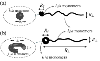
Figure 1: Schematic representations of a polymer in the folding process at $l_{p}\approx a$ (a) and $l_{p}\gg a$ (b). The polymer consists of collapsed and coiled domains. The collapsed domain has $l_{1}/a$ monomers and the size $R_{\rm f}$. The coiled domain has $l_{2}/a$ monomers and the lateral fluctuation $R_{\perp}$.

III.1 nucleation for a flexible chain ($l_{p}\approx a$)

When a polymer is flexible, i.e., $l_{p}\approx a$, it collapses into a disordered globule. Since, in the collapsed state, the mean field approximation is applicable, the total free energy is written approximately with the contributions from the surface, bending, and volume free energies as

$$F_{\rm collapse} = F_{\rm surface}+F_{\rm bend}+F_{\rm volume}$$ (9)

$$\simeq \sigma R_{\rm f}^{2}+\kappa\frac{l_{1}}{R_{\rm f}^{2}}-\epsilon l_{1},$$ (10)

where $\sigma$ and $\epsilon$ are the surface tension and interaction energy density, respectively, and $R_{f}\simeq(l_{1}a^{2})^{1/3}$. We use the relation between the bending constant and the persistence length: $\kappa/T=l_{p}$. The free energy change is

$$\frac{{\rm d}F}{{\rm d}t}\simeq\left[\frac{\sigma a^{4/3}}{l_{1}^{1/3}}+\frac{Tl_{p}}{l_{1}^{2/3}a^{4/3}}-\epsilon\right]\left(\frac{{\rm d}l_{1}}{{\rm d}t}\right).$$ (11)

Because the dissipation is an irreversible process, the sign of ${\rm d}l_{1}/{\rm d}t$ is determined by the free energy change. Therefore, the critical size of a nucleus is calculated as

$$l_{1}^{*}\simeq\left(\frac{\sigma}{\epsilon}\right)^{3}a^{4}+\frac{3\sigma Tl_{p}}{\epsilon^{2}}.$$ (12)

The free energy at this size corresponds to the barrier between the coiled and collapsed states, and the characteristic time for the nucleation process $\tau_{c}$ exponentially depends on it. In addition, $\tau_{c}$ weakly depends on the dissipation rate because it determines the velocity of the growth of a nucleus. We obtain the nucleation time for a disordered collapse as

$$\tau_{c}\simeq\frac{\tilde{\gamma}^{*}}{\sigma}\left(\frac{l_{1}^{*}}{a}\right)^{4/3}\exp\left[\frac{\sigma^{3}a^{4}}{\epsilon^{2}T}+\frac{3\sigma l_{p}}{\epsilon}\right],$$ (13)

where $\tilde{\gamma}^{*}=\tilde{\gamma}(l_{1}=l_{1}^{*})$ is the effective friction at the critical nucleus. The prefactor arises from second derivative of free energy at critical size of nucleus. The details of the prefactor depend on the dissipation mechanism which is discussed below. Nevertheless, the nucleation time is essentially dominated by the exponential factor.

III.2 nucleation for a semiflexible chain ($l_{p}\gg a$)

The free energy of a collapsed domain depends on its structure and here we consider a toroidal conformation (Fig. 1). The free energy is expressed as the summation of the surface, bending and volume energies,

$$F_{\rm collapse}^{\rm toroid}\simeq\sigma rR_{\rm f}+\kappa\frac{l_{1}}{R_{\rm f}^{2}}-\epsilon l_{1}.$$ (14)

The surface and bending energies are balanced; as a result, with the condition of the closely packed conformation in the folded part $2\pi^{2}r^{2}R_{\rm f}=l_{1}a^{2}$, the free energy change is estimated as

$$\left(\frac{{\rm d}F}{{\rm d}t}\right)_{\rm collapse}^{\rm toroid}\simeq\left[\left(\frac{\sigma^{4}l_{p}Ta^{4}}{l_{1}^{2}}\right)^{1/5}-\epsilon\right]\left(\frac{{\rm d}l_{1}}{{\rm d}t}\right).$$ (15)

We obtain the following nucleation time for ordered collapse:

$$\tau_{c}\simeq\frac{\tilde{\gamma}^{*}l_{1}^{*7/5}}{(\sigma^{4}l_{p}Ta^{4})^{1/5}}e^{\epsilon l_{1}^{*}},$$ (16)

where $l_{1}^{*}=\sigma^{2}l_{p}^{1/2}/\epsilon^{5/2}$.

III.3 growth

In the growth step, the force $f$, given by (8), that pulls the monomers in the coiled domain is balanced by the effective frictional force arising from dissipation:

$$\tilde{\gamma}v=f,$$ (17)

where $v=\mathrm{d}l_{1}/\mathrm{d}t=-\mathrm{d}l_{2}/\mathrm{d}t$. The absorbing force of Eq.(8), arising from free energy change, is essentially,

$$f\simeq\epsilon,$$ (18)

where we neglect the contribution of the surface term, which is sufficiently small at $l_{1}\gg a$. The effective friction depends on the dissipation mechanism, and therefore, in general, would depend on the conformation of a chain. The above force-balance relation is nothing but energy balance in (1) as can be confirmed by multiplying both sizes by $\mathrm{d}l_{1}/\mathrm{d}t$.

Let us consider the conformation shown in Fig. 1 just after nucleation. The collapsed domain is pulled by the coiled domain with $f$ and vice versa. The system is similar to the relaxation of stretched polymersBrochard-Wyart et al. (1994); Hallatschek et al. (2005) and adsorption of polymers by pulling on end with external force Grosberg et al. (2006); Sakaue (2007). In the former system, flexible Brochard-Wyart et al. (1994) and semiflexible Hallatschek et al. (2005) polymers are stretched when a force is applied at one or two ends. In the latter systems, a polymer is pulled at a constant force and is absorbed into a pore. In both systems, after the force is switched on, tension propagates along a chain with finite velocity. Therefore, not all the monomers move by the force, but some parts are driven by the force and others do not feel it. The results of these works show that the effective friction depends on the length of monomers moving under force, and their motion is initiated by the propagation of the force.

In our system, the force is acting on the interface between collapsed and coil domains. While the force quickly propagates on the entire collapsed domain due to the cooperative motion of monomers, the force acting on the coil domain propagates with some velocity. The time required for propagation is not infinitesimal. The overall motion of a chain does not contribute to the effective friction, but relative motion of a collapsed or coil domain leads to dissipation. Thus, the question arises in the growth step: which domain moves? This is equivalent to asking which domain contributes to dissipation. Since in the free-drain limit, friction is proportional to the length of a moving domain, the collapsed domain moves quickly and makes a dominant contribution, at least, at an early stage of the growth step. At a later stage, when the length of a collapsed domain becomes much longer than that of a coil domain, and in addition, when the force propagates to the free end of the coil domain, the coiled domain makes dominant contribution to dissipation. Therefore, we assume that the dominant contribution is from the collapsed domain at the early stage. The effective frictional coefficient is described in the free-drain limit as

$$\tilde{\gamma}\simeq\gamma_{1}=\eta l_{1}.$$ (19)

In semiflexible polymers, the logarithmic correction $(\ln(l_{p}/a))^{-1}$ is multiplied on the right-hand side. At the later stage after force propagation, the effective friction is described as

$$\tilde{\gamma}\simeq\gamma_{2}=\eta(L-l_{1}).$$ (20)

Therefore, the velocity is

$$v\simeq\left(\frac{1}{\gamma_{1}}+\frac{1}{\gamma_{2}}\right)f=\frac{\epsilon L}{\eta l_{1}(L-l_{1})},$$ (21)

where we neglect the logarithmic correction. Note that this argument is justified even with hydrodynamic interaction. We will see this in section VI.

IV Unfolding Transition

When, at $t=0$, the attractive interaction is switched off, a collapsed polymer starts to unfold. While, in the folding transition, the kinetics is dominated by the competition between the free energies that do and do not prefer the collapsed state, in the unfolding transition all the terms in the free energy make a collapsed polymer unfold. In fact, the free energies of the entropic elasticity, the bending elasticity, and the excluded volume interaction are larger in the folded state. This suggests that the collapsed state is unstable at an early stage of the transition. After the swelling step, the structure is similar to a coiled state, but it has many entanglements, which are expected to lead to slow kinetics. Finally, a polymer relaxes into an equilibrium coiled state. Therefore, we assume that the unfolding process consists of three steps: swelling, disentanglement, and relaxation (fig. 2).

In the unfolding transition, the free energy is described with elastic and interaction terms.

$$F\simeq T(\alpha^{2}+\alpha^{-2})+\frac{B}{R_{L}^{3}}\left(\frac{L}{l_{p}}\right)^{2},$$ (22)

where $\alpha=R_{L}/(Ll_{p})^{1/2}$, and $B\simeq l_{p}a^{2}T(1-\Theta/T)$ is the second virial coefficient. $\Theta$ is the critical temperature of the transition. At $t=0$, we increase the temperature so that $B\simeq l_{p}a^{2}T>0$. In the entropic contribution, the first term shows energy penalty for expansion and the second term corresponds to that for compression. Here we consider relaxation to an equilibrium coiled state, i.e., the second term is dominant. The volume interaction is dominant at the swelling step and almost disappears after the step. In the disentanglement and relaxation steps, we consider the free energy change due to the entropic contribution in Eq. (22).

IV.1 Swelling

In this step, the dominant contribution of interactions between monomers gives the free energy change,

$$\frac{{\rm d}F}{{\rm d}t}\simeq\left(-\frac{BL^{2}}{R_{L}^{4}l_{p}^{2}}\right)\frac{{\rm d}R_{L}}{{\rm d}t}.$$ (23)

The dissipation arises from all the monomers and is described as,

$$\frac{{\rm d}Q_{\rm S}}{{\rm d}t}\simeq\eta\frac{L}{l_{p}}\frac{l_{p}}{\ln(l_{p}/a)}\left(\frac{{\rm d}R_{L}}{{\rm d}t}\right)^{2}.$$ (24)

With Eq. (1), the time evolution is given by

$$\frac{R_{L}}{R_{\rm swell}}\simeq\left(1+\frac{|B|L}{l_{p}^{2}R_{\rm swell}^{5}}t\right)^{1/5},$$ (25)

where $R_{\rm swell}$ is the size in folded states.

Since monomer-monomer interaction is short ranged (the length scale is $\delta=\mathcal{O}(a)$), this regime is over when the mean distance between monomers exceeds $\delta$. Therefore, the characteristic time is

$$\tau_{\rm swell}\simeq\frac{L^{2/3}l_{p}}{\ln(l_{p}/a)a^{5/3}}\tau_{0},$$ (26)

where we use the microscopic time scale $\tau_{0}=\eta a^{3}/k_{B}T$. As we will see later, this time scale ($\sim L^{2/3}$) is much shorter than the time scale of other two regimes. We conclude that the swelling regime does not exhibit dynamic scaling behaviors.

IV.2 Disentanglement

In the steps of disentanglement and relaxation, the free energy change originates from the elastic free energy, which is given by

$$\frac{{\rm d}F_{\rm ela}}{{\rm d}t}\simeq-\frac{T}{\alpha^{3}}\frac{{\rm d}\alpha}{{\rm d}t}.$$ (27)

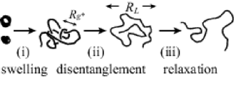
Figure 2: Three steps in the unfolding process. (i) swelling, (ii) disentanglement, and (iii) relaxation. We characterize the time evolution with the size $R_{L}$.

For the conformation with entanglements, a topological blob, which consist of $g^{*}l_{p}$ monomers and is $R_{g^{*}}$ in size can be defined Grosberg et al. (1988). Inside a topological blob, a chain behaves like a Gaussian coil, whereas on a larger scale, a chain is assumed as a swollen globule. Therefore, $R_{g^{*}}^{2}\sim g^{*}l_{p}^{2}$ and $g^{*}l_{p}/R_{g^{*}}^{3}\sim L/R_{L}^{3}$ is satisfied. This leads to the following relations:

$$g^{*}\simeq\frac{R_{L}^{6}}{L^{2}l_{p}^{4}},$$ (28)

$$R_{g^{*}}\simeq\left(\frac{l_{p}g^{*}}{L}\right)^{1/3}R_{L}.$$ (29)

Beyond the scale, blobs are frozen due to entanglements and behave as obstacles when monomers in a particular blob are driven. Since we neglect the hydrodynamic interactions, the dissipation inside a blob is proportional to the number of segments $g^{*}$, and it is written in the free-drain limit as

$$\frac{{\rm d}Q_{\rm S}}{{\rm d}t}\simeq\frac{L^{2}}{l_{p}^{2}g^{*}}\eta g^{*}\frac{l_{p}}{\ln(l_{p}/a)}\left(\frac{{\rm d}R_{g^{*}}}{{\rm d}t}\right)^{2}\simeq\eta\frac{R_{L}^{4}}{l_{p}^{3}\ln(l_{p}/a)}\left(\frac{{\rm d}R_{L}}{{\rm d}t}\right)^{2}.$$ (30)

From the energy balance, we obtain

$$\frac{R_{L}}{R_{\rm dis}} \simeq \left(\frac{t}{\tau_{\rm dis}}+1\right)^{1/8},$$ (31)

$$\tau_{\rm dis} \simeq \frac{L^{5/3}l_{p}^{4/3}}{a^{3}\ln(l_{p}/a)}\tau_{0},$$ (32)

where $R_{\rm dis}\simeq L^{1/3}l_{p}^{2/3}$ are the initial value and $\tau_{\rm dis}$ is the characteristic time scale, respectively, in this regime. We have assumed the swollen globular structure for the initial state. For $t\gg\tau_{\rm dis}$, the following scaling relation is obtained;

$$R_{L}\sim t^{1/8}.$$ (33)

This step proceeds during $g^{*}\ll L/l_{p}$, where a polymer has many entanglements so that we assume the outside of blobs to be frozen. The characteristic time scale of this step is obtained with the condition $g^{*}=L/l_{p}$ and is proportional to $L^{3}$, which is much longer than the time scales of the other two steps.

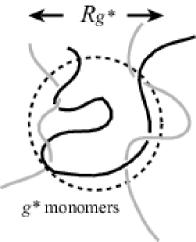
Figure 3: Schematic representation of a topological blob of $g^{*}$ monomers. Inside a blob, a polymer behaves as a coil, whereas it is entangled on a larger scale.

IV.3 Relaxation

Contrary to the disentanglement step, in the relaxation step, all segments contribute to dissipation, and thus, it is given as

$$\frac{{\rm d}Q_{\rm S}}{{\rm d}t}\simeq\eta\frac{L}{l_{p}}\frac{l_{p}}{\ln(l_{p}/a)}\left(\frac{{\rm d}R_{L}}{{\rm d}t}\right)^{2}.$$ (34)

From Eqs. (27) and (34), we obtain

$$\frac{R_{L}}{R_{\rm relax}} \simeq \left(\frac{t}{\tau_{\rm relax}}+1\right)^{1/4},$$ (35)

$$\tau_{\rm relax} \simeq \frac{L^{2}l_{p}}{a^{3}\ln(l_{p}/a)}\tau_{0},$$ (36)

where $R_{\rm relax}\sim(Ll_{p})^{1/2}$ and $\tau_{\rm relax}$ are the initial value and the characteristic time scale, respectively, in the relaxation step. We estimate $R_{\rm relax}$ from the condition $g^{*}=L/l_{p}$. We should note that the feature of $\tau_{\rm relax}\sim L^{2}$ is typical in the Rouse dynamics Doi and Edwards (1986). For $t\gg\tau_{\rm relax}$, the following scaling relation is obtained:

$$R_{L}\sim t^{1/4}.$$ (37)

V Simulations

In order to examine the folding and unfolding kinetics, we carried out Langevin dynamics simulations of a bead-spring model using the following potentials:

$$V_{\mathrm{beads}} = \frac{k_{a}}{2}\sum_{i}({|\mathbf{r}_{i+1}-\mathbf{r}_{i}|}-a)^{2},$$ (38)

$$V_{\mathrm{bend}} = \frac{\kappa}{2}\sum_{i}(1-\cos\theta_{i}),$$ (39)

$$V_{\mathrm{LJ}} = 4\epsilon_{\mathrm{LJ}}\sum_{i,j}\left[\left(\frac{a}{|\mathbf{r}_{i}-\mathbf{r}_{j}|}\right)^{12}-\left(\frac{a}{|\mathbf{r}_{i}-\mathbf{r}_{j}|}\right)^{6}\right],$$ (40)

where $V=V_{\mathrm{beads}}+V_{\mathrm{bend}}+V_{\mathrm{LJ}}$, and $\mathbf{r}_{i}$ is the coordinate of the $i$th monomer, and $\theta_{i}$ is the angle between adjacent bond vectors. The monomer size $a$ and $k_{B}T$ are chosen as the unit length and energy, respectively. Monomer-monomer interactions are included with the Lennard-Jones potential, $V_{\mathrm{LJ}}$, which contains the soft-core excluded volume interaction and the short-ranged attractive interaction. With small $\epsilon_{\mathrm{LJ}}$, the attraction is week such that only the excluded volume interaction is relevant. We set $\epsilon_{\mathrm{LJ}}=0.3$ for this good solvent condition. On the other hand, with large $\epsilon_{\mathrm{LJ}}$, the attractive interaction plays a role for the folding transition (poor solvent condition). We adopt the spring constant in $V_{\mathrm{beads}}$ to be $k_{a}=400$. The persistence length $l_{p}$ is a convenient measure to characterize the stiffness of a polymer chain. The bending elasticity $\kappa$ in $V_{\mathrm{bend}}$ satisfies the relation $\kappa=l_{p}T$. We consider a homopolymer mainly with a polymerization index $N=256$, which has sufficient length for the formation of ordered structures (a toroid, a cylinder, and so on) in a semiflexible polymer Noguchi et al. (1996).

The equation of motion is written as

$$m\frac{{\mathrm{d}}^{2}{\mathbf{r}}_{i}}{{\mathrm{d}}t^{2}}=-\gamma\frac{{\mathrm{d}}{\mathbf{r}}_{i}}{{\mathrm{d}}t}-\frac{\partial V}{\partial{\mathbf{r}}_{i}}+{\boldsymbol{\xi}}_{i},$$ (41)

where $m$ and $\gamma$ are the mass and friction constant of monomeric units, respectively. The unit time scale is $\tau_{0}^{s}=\gamma a^{2}/k_{B}T=6\pi\tau_{0}$. We set the time step as $0.01\tau_{0}^{s}$ and use $m=1.0$ and $\gamma=1.0$. With these parameters, the relaxation time of the momentum of a monomer is sufficiently fast as compared to the time scale of interest. Gaussian white noise ${\boldsymbol{\xi_{i}}}$ satisfies the following fluctuation-dissipation relation:

$$<{\boldsymbol{\xi}}_{i}(t)\cdot{\boldsymbol{\xi}}_{j}(t^{\prime})>=6\gamma k_{B}T\delta_{ij}\delta(t-t^{\prime}).$$ (42)

The folding and unfolding states of a polymer are characterized by the number of folded monomers $N_{\rm{fold}}$, which is defined by

$$\rho_{i} = \sum_{j}H(r_{c}^{2}-|{\mathbf{r}}_{i}-{\mathbf{r}}_{j}|^{2}),$$ (43)

$$N_{\rm{fold}} = \sum_{i}\Theta(\rho_{i}-\rho_{c}),$$ (44)

where $H(x)$ and $\Theta(x)$ are the Heaviside and Step functions, respectively, and $\rho_{i}$ is the local monomer density. In this work, we set $r_{c}=3.0$ and $\rho_{c}=25.0$. The nucleation time, $\tau_{c}$, is defined so as to satisfy $N_{\rm{fold}}(\tau)\geq N_{c}$ for $\tau\geq\tau_{c}$, where we set $N_{c}=0.20$. We should note that our results do not depend on these specific values. Conformations of a polymer are characterized with the long-axis length,

$$R_{L}=\max|{\bf r}_{i}-{\bf r}_{j}|.$$ (45)

In the folding transition, coiled polymers were equilibrated under the good solvent condition, $\epsilon_{\mathrm{LJ}}=0.30$, and then quenched at $t=0$ into the poor solvent conditions such as $\epsilon_{\mathrm{LJ}}=0.70$, $1.0$, and $1.3$. Although we had various structures such as a toroid and a rod for $l_{p}\geq 10a$, we chose toroidal conformations, and the macroscopic variables were averaged over the ensemble of this conformation for consistency with our theory. To achieve this, we neglected the trajectories whose final conformations have the long-axis length larger than $20a$ in order to ensure that the final conformations are the troidal state. Typically, cylindrical conformations have a size of more than $20a$ in the folded state. In the unfolding transition, we prepared folded polymers at $\epsilon_{\mathrm{LJ}}=1.0$, and quenched the system at $t=0$ into $\epsilon_{\mathrm{LJ}}=0.30$. We calculated the fraction of collapsed part and averaged it over more than 100 runs.

Figure 4 shows the typical time evolution of the ratio of monomers in the folded state. As we can see, after a long lag time, the ratio increases with time and reaches the equilibrium value.

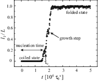
Figure 4: Typical time evolution of $l_{1}$ in the folding transition. The attractive interactions switch on at $t=0$ by replacing $\epsilon=0.3$ with $\epsilon=1.0$.

The dependence of the nucleation time on the persistence length is shown in Fig. 5. For small $l_{p}$, the nucleation time exponentially depends on the persistence length, which is consistent with Eq. (13). For large $l_{p}$, the slope becomes rather gentle. This is also consistent with our theory of Eq. (16), where $\tau_{c}\sim\exp(l_{p}^{1/2})$.

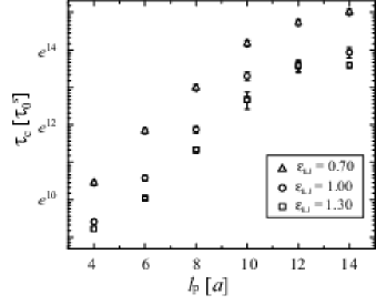
Figure 5: A semi-log plot of nucleation time as a function of persistence length.

The velocity of $l_{1}$ after nucleation is plotted in fig. 6, where the velocity is inversely proportional to $l_{1}$. This implies that friction does not arise from the coil part. If the coil domain involves friction, the velocity will increases with $l_{1}$. In the section III C, we discussed velocity of the growth step, which is valid early and later stages. At the early stage, $v\sim\epsilon/(\eta l_{1})$ while at the later stage, $v\sim\epsilon/(\eta(L-l_{1}))$. Our results of simulations are consistent with (21) at the early stage. However, at the later stage, our theory predict increase of velocity. The discrepancy may be explained with large fluctuation of the fraction of folded monomers. In fact, the system reaches at the folded state even at $l_{1}/L<1$ as shown in Fig. 6B. Since the driving force for the folding transition decreases close to the equilibrium state, velocity near $l_{1}/L\approx 1$ is expected to decrease as in Fig. 6. In our theory, we assume that driving force is constant throughout the growth step.

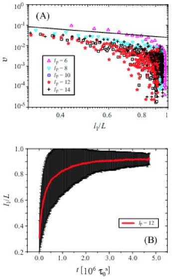
Figure 6: (A) A log-log plot of velocity during growth steps. The line shows $v\sim l_{1}^{-1}$. (B) Mean value and fluctuation of the fraction of the folded state with $l_{p}=12$.

Let us now discuss the unfolding transition. First, we show the result of a relatively long ($N=2048$) chain. Figure 7 shows that there indeed exists slow kinetics after the swelling step. The slow kinetics is independent of the interaction energy, while the swelling step is characterized by the interaction energy (Fig. 7(B)). The LJ potential contains a weak attractive part even in the coil state. Since the interaction is short-ranged, the energy is approximately 0 in the coil state. This is shown in Fig. 7B. The system is not in equilibrium even at $10^{8}\tau^{s}_{0}$, which is much longer than the Rouse time ($\simeq 10^{6}-10^{7}$). On the other hand, an ideal polymer is equilibrated much faster, as expected. Thus, it is evident that slow kinetics exist in the unfolding transition, and this fact is due to the non-crossing constraint of a chain with excluded volume interaction. Note that the slow kinetics was also observed in the simulations of flexible polymers in Byrne et al. (1995). Since computation with long chains is time consuming to obtain statistics, we used $N=256$ chains and took average over 100 runs. Figure 8 and 9 shows the results of the unfolding transition. The size and time are normalized with characteristic space and time scales according to Eq. (32) for an early stage and Eqs. (35) and (36), respectively, for a later stage. The initial size for the disentanglement step is determined from the result of simulations. Since the swelling process for N=256 chains is short ($\simeq 10^{3}$ steps), the value of $R_{1}$ corresponds to $R_{L}$ after a jump at $t>0$ ( Fig. 8A). The time evolution of the long-axis length exhibits a universal feature in which the plots do not qualitatively depend on the persistence length and the depth of quench. In addition, the data cover from $t\simeq\tau$ to $t\gg\tau$, and thus our simulations have a suitable time scale. In both figures, the slopes are in good agreement with our theory.

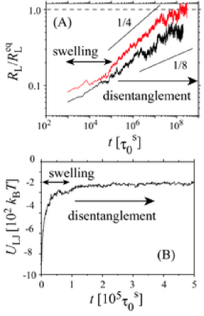
Figure 7: Time evolution of a long chain ($N=2048$) during the unfolding transition. (A) Time evolution shows slow relaxation after initial expansion (the lower black line). The size is normalized with the equilibrium size, $R^{\rm eq}_{\rm L}$. The both axes are shown with logarithmic scale. The kinetics of an ideal polymer is also shown (the upper red line). (B) Interaction between monomers quickly decreases at an early stage of the transition. The two solid lines show $t^{1/4}$ and $t^{1/8}$. The size at the equilibrium state is estimated from the additional simulations at a fixed value of epsilon.

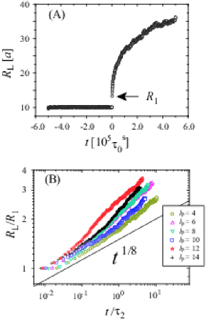
Figure 8: Time evolution of the long-axis length of a polymer at an early stage for various persistence length. Bare plot for $l_{p}=4$ is shown in (A). We determine the initial values for the disentanglement process from $R_{1}$ in the figure. (B) A log-log plot of the time evolution. Both the long-axis length and time steps are normalized with characteristic space and time scales (see Eqs. (33)).

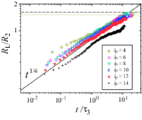
Figure 9: A log-log plot of time evolution of the long-axis length of a polymer at a later stage for various persistence length. Both the long-axis length and time steps are normalized with characteristic space and time scales according to Eq. (37) in the text. The dashed and dotted lines show the equilibrium size for $l_{p}=4$ and $l_{p}=14$, respectively.

VI Hydrodynamics

With the hydrodynamic interaction our previous theory is modified depending on their kinetics. For expansion and contraction of a domain, it is necessary to consider the dissipation of Eq. (3). For cooperative motion of monomers, the modified Stokes dissipation due to hydrodynamic back flow is applied. The Stokes drag does not act on each segment, but acts on a sphere of $\xi_{\rm H}$ in size, while hydrodynamic interactions are screened beyond the screening length. At a length scale smaller than $\xi_{\rm H}$, monomers move cooperatively with the hydrodynamic back flow. Thus, the dissipation is

$$\frac{{\rm d}Q_{\rm S}}{{\rm d}t}\simeq\eta v^{2}\xi_{\rm H}.$$ (46)

This feature is called as non-drain compared with the situation of free-drain where all monomers are under the Stokes drag de Gennes (1976); Ahlrichs et al. (2001).

VI.1 Folding Transition

The kinetics of the folding transition essentially does not change in the nucleation process with hydrodynamic interaction since dissipation modifies the prefactors of the nucleation time in Eqs. (13) and (16). On the other hand, in the growth process, the friction of a chain is proportional to its size. Therefore, the collapsed part has smaller friction, which is proportional to $l_{1}^{1/3}$, for example, for flexible polymers. The friction is much smaller than that of the coiled domain; thus, it supports the assumption that only the collapsed domain contributes to the dissipation in the growth step. We obtain the velocity as

$$v=\frac{\epsilon}{\eta a^{2/3}}\frac{1}{l_{1}^{1/3}}$$ (47)

for flexible polymers, and

$$v=\frac{\epsilon}{\eta}\left(\frac{\sigma a}{Tl_{p}}\right)^{2/5}\frac{1}{l_{1}^{1/5}}$$ (48)

for semiflexible polymers.

VI.2 Unfolding Transition

In the initial stage of the unfolding transition, the hydrodynamic interaction is approximately screened, while in the disentanglement and the relaxation regimes, the hydrodynamic interaction is relevant to the kinetics of the transition. In the disentanglement process, the hydrodynamic interaction is screened outside blobs since the blobs are pinned due to entanglements. The dissipation inside a blob is

$$\frac{\mathrm{d}Q_{H}}{\mathrm{d}t} \simeq \left(\frac{L}{l_{p}g^{*}}\right)^{2}\eta R_{g}\left(\frac{\mathrm{d}R_{g}}{\mathrm{d}t}\right)^{2}$$ (49)

$$= \eta\frac{L^{3}l_{p}^{3}}{R_{L}^{5}}\left(\frac{\mathrm{d}R_{L}}{\mathrm{d}t}\right)^{2}.$$ (50)

We obtain

$$\left(\frac{R_{L}}{R_{disent}}\right)^{-1} = 1-t/\tau_{\rm disentangle}$$ (51)

$$\tau^{\prime}_{\rm disentangle} = =\frac{\eta L^{5/3}l_{p}^{4/3}}{a^{3}}\tau_{0}.$$ (52)

In the relaxation regime, hydrodynamic back flow dominates the entire polymer. Thus, the dissipation is

$$\frac{{\rm d}Q_{\rm H}}{{\rm d}t}\simeq\eta R_{L}\left(\frac{{\rm d}R_{L}}{{\rm d}t}\right)^{2}.$$ (53)

By using Eqs. (1), (27), and (53), we obtain

$$\frac{R_{L}}{R_{\rm relax}} \simeq \left(\frac{t}{\tau^{\prime}_{\rm relax}}+1\right)^{1/5},$$ (54)

$$\tau^{\prime}_{\rm relax} = \eta(Ll_{p})^{3/2}.$$ (55)

Here, the characteristic time scale has the Zimm-type feature, $\tau^{\prime}_{\rm relax}\sim L^{3/2}$ Doi and Edwards (1986).

VII Kinetic pathway

In our theory, we assume that the kinetic pathway is nucleation and growth for the folding process (Fig.10a) and gradual expansion for the unfolding process (Fig.10c). However, we may also assume the opposite pathway, i.e., gradual contraction for the folding process (Fig.10d) and nucleation and growth process for the unfolding process (Fig.10c). Here, we discuss the reason for why the later pathway does not appear. An importance fact is that a faster process at the initial stage of the transition is able to survive. We will calculate the time evolution of the unrealistic pathways (Fig. 10b and d) and compare it with the results we obtained. For simplicity, we will discuss kinetics without the hydrodynamic interaction.

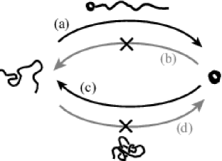
Figure 10: Kinetic pathways of the folding and unfolding transitions. We assume (a) and (c) since the pathways (b) and (d) are unrealistic, as shown in the text.

VII.1 Folding transition

Here, we consider an early stage of the kinetics of Fig. 10(d). In the process, the free energy change is divided into two terms: the elastic and the volume free energy. The former prevents the folding transition, while the later initiates the transition. The volume free energy is written as

$$F_{\rm int}\simeq\frac{B}{R_{L}^{3}}\left(\frac{L}{l_{p}}\right)^{2}.$$ (56)

At $t=0$, we decrease the temperature so that $B<0$. The free energy change is calculated as

$$\frac{{\rm d}F}{{\rm d}t}\simeq\left(-\frac{BL^{2}}{R_{L}^{4}l_{p}^{2}}-\frac{TLl_{p}}{R_{L}^{3}}\right)\frac{{\rm d}R_{L}}{{\rm d}t},$$ (57)

where the second term is the contribution of the elastic free energy. The first term contributes to decrease the free energy, while the second makes a opposite contribution. When $R_{L}$ is close to the equilibrium size in the swollen state $\simeq(Ll_{p})^{1/2}$, the first term is proportional to $\sim L^{0}$ and the second term is proportional to $\sim L^{-1/2}$. We are interested in the kinetics of the early stage of this pathway. Thus, we neglect the second term in (57). The dissipation in this process is

$$\frac{{\rm d}Q_{\rm S}}{{\rm d}t}\simeq\eta L\left(\frac{{\rm d}R_{L}}{{\rm d}t}\right)^{2},$$ (58)

where we neglect logarithmic factor for simplicity. With Eq. (1), the time evolution is

$$\frac{R_{L}}{R_{2}}\simeq\left(1-\frac{|B|L}{l_{p}^{2}R_{2}^{5}}t\right)^{1/5}.$$ (59)

At the early stage, the time evolution is

$$R_{L}\simeq R_{2}-\frac{|B|L}{l_{p}^{2}R_{2}^{4}}t,$$ (60)

where the velocity is proportional to $L^{-1}$. Thus, we expect this process to be too slow to proceed before the nucleation process.

VII.2 Unfolding transition

In the unfolding transition, we may assume the kinetic pathway of Fig. 10(b), that is, the collapsed polymer with a short unfolded coiled part. The kinetics is driven by the free energy change of the peeled part, which is in fact the difference of the free energy between the coiled and the collapsed states:

$$\frac{\mathrm{d}F}{\mathrm{d}t}\simeq-\frac{T}{l^{2/3}l_{p}^{1/3}}\frac{\mathrm{d}l}{\mathrm{d}t}.$$ (61)

The dissipation from the coiled part is

$$\frac{\mathrm{d}Q}{\mathrm{d}t}\simeq\eta l\left(\frac{\mathrm{d}l}{\mathrm{d}t}\right)^{2}.$$ (62)

Therefore, we obtain

$$l\simeq\left(\frac{T^{3}}{\eta^{3}l_{p}}\right)^{1/8}t^{3/8},$$ (63)

which indicates that the characteristic time for this pathway is proportional to $L^{8/3}$. As in section IV, the swelling regime proceeds much faster. From this, we conclude that the pathway is not realized.

VIII Summary and Remarks

In summary, we investigated the kinetics of the folding and unfolding transitions in a single semiflexible polymer with and without the hydrodynamic interaction. We found that the velocity of the length of the collapsed domain depends inversely on the length in the folding transition, and the dynamic scaling exponents are $1/8$ and $1/4$ for the disentanglement and relaxation steps, respectively, in the unfolding transition without the hydrodynamic interaction. The time dependence without the hydrodynamic interaction is also calculated using Langevin Dynamics simulations, is found to be in good agreement with our theory.

We discussed the origin of dissipation during the folding and unfolding transitions. The main contribution in the folding transition is found to be the motion of the collapsed domain along a chain. We proposed a slow relaxation regime in the unfolding transition arising from entanglements of a polymer. Since this regime is not found in an ideal polymer, we consider that the slow kinetics originate from the topological constraint due to the excluded volume interaction.

Although the kinetics of single semiflexible polymers have not been studied extensively in experiments, the authors in ref. Yoshikawa and Matsuzawa (1996); Ichikawa et al. (2005) investigated the time evolution of long DNA molecules by using fluorescent microscopy. In Ichikawa et al. (2005), DNA molecules were contracted using optical tweezers under good solvent conditions. After switching the optical tweezers off, the time evolution of the size of DNA molecules was observed, and small exponent of 0.125 was found. This result corresponds well with the disentanglement regime in our results. In Yoshikawa and Matsuzawa (1996), the transitions were induced by a sudden change in the concentration of multivalent cations. In the folding transition, they found linear time dependence of the apparent size of a DNA molecule. Since the data have large fluctuations, quantitative comparison is difficult at the moment. Nevertheless, we believe that further experimental studies would be helpful for comparison between theory and experiments.

To conclude this paper, we make some remarks for future investigations.

1. We have considered single nucleation along a chain. This is a limited situation because nucleation usually occurs simultaneously along a chain. However, as we discussed, the nucleation time depends exponentially on the persistence length. This indicates that we need a very long chain to obtain multiple nucleations with a large persistence length. This is in contrast to the case of flexible polymers where multiple nucleations called pearl-necklace structure dominates at an early stage of the folding transition Klushin (1998); Halperin and Goldbart (2000). We should note that when we have a very long semiflexible chain, we should consider a network structure rather than multiple nucleations along a chain since nucleation does not occur locally due to the bending rigidity.

2. As noted in introduction, we have concentrated on the toroidal structure. This makes the problem tractable. To discuss further, we have to consider cylindrical conformations. They appear as the equilibrium state in a range of parameters, but the difficulty is that they have many metastable structures depending on the number of times they are folded. Cylinders that are few times folded are likely to appear in the kinetics though they are not equilibrium structure but metastable states. After certain time, they become more folded structures or sometimes make a transition into toroidal structures. The kinetics of folding into cylindrical conformations are dominated by such hopping steps, which are different from the kinetics for toroidal conformations. It is interesting, as a further study, to discuss the bifurcation between the two kinetics, the nucleation and growth, which are discussed in the present work, and hopping steps found in kinetics of cylindrical collapses.

3. Our calculation of the nucleation time is qualitative. In order to make quantitative discussions, it is necessary to take loop formation into account. In fact, the nucleation process initiates with loop formation Hyeon and Thirumalai (2006). This modifies the prefactors in the nucleation time Eqs. (13) and (16). Nevertheless, the nucleation time is dominated by the exponential factor. Therefore, we expect our results to be qualitatively reasonable.

4. Our comparison between theory and simulation is under the condition without the hydrodynamic interaction. Recently, several algorithms have become available to deal with the hydrodynamic interaction in polymer systems. For example, Stochastic Rotation Dynamics Kikuchi et al. (2002, 2005) and Lattice Boltzmann Dünweg (2004) were implemented for investigating the kinetics of polymers. Such simulations would reveal details of the physical processes involved in the kinetics of the folding and unfolding transitions when the hydrodynamic interaction is also considered, and would test the validity of our theory.

5. Quantitative arguments for the disentanglement process are still left as a future study. In particular, the crossover between disentangled and swollen states is not clear. We should note that the characteristic time in this study is overestimated. In fact, disentanglement process does not end at $g^{*}\simeq L/l_{p}$, but is replaced earlier by the relaxation process since topological blobs suddenly disappear when they become sufficiently large. Our theory does not include such effects.