Eigenvectors of the discrete Laplacian on regular graphs - a statistical approach

Abstract

In an attempt to characterize the structure of eigenvectors of random regular graphs, we investigate the correlations between the components of the eigenvectors associated to different vertices. In addition, we provide numerical observations, suggesting that the eigenvectors follow a Gaussian distribution. Following this assumption, we reconstruct some properties of the nodal structure which were observed in numerical simulations, but were not explained so far [1]. We also show that some statistical properties of the nodal pattern cannot be described in terms of a percolation model, as opposed to the suggested correspondence [2] for eigenvectors of 2 dimensional manifolds.

1 Introduction

In the past few decades, the spectral properties of regular graphs had attracted considerable attention of researchers from diverse disciplines such as combinatorics, information theory, theoretical and applied computer science, quantum chaos and spectral theory (to list only a few). In order to understand better the eigenvectors of the Laplacian on such graphs, we try to establish some analogies between those eigenvectors, to eigenvectors of chaotic manifolds. The tools we are using for this task, are mostly probabilistic.
In the following, we consider the statistical properties of $G(n,d)=(V,E)$ - a graph which is chosen uniformly at random from the set of $d-$regular graphs on $n$ vertices. The graph can be uniquely described by its adjacency matrix $A$ (also known as the connectivity matrix), where $A_{i,j}=1$ if $v_{i}$ and $v_{j}$ are adjacent vertices in $G$, or zero otherwise. The action of the discrete Laplacian on a function $f:V\rightarrow\mathbb{R}$ is

$$Lf_{i}=\sum_{i\sim j}(f_{i}-f_{j})$$ (1)

where $f_{i}\equiv f(v_{i})$, and the summation is over all vertices $v_{j}$ which are adjacent to $v_{i}$. For regular graphs, the Laplacian can be expressed in a matrix form as $L=dI-A$, therefore an eigenvector of the Adjacency matrix with an eigenvalue $\lambda$, is also an eigenvector of the Laplacian, with an eigenvalue $\mu=d-\lambda$.
The eigenvalues and eigenvectors of $A$ contain valuable information about the structure of the graph. The relations between the spectrum of the adjacency matrix to the expansion properties of $G$ (see section 2.2), have been thoroughly investigated and were found useful for coping with a variety of tasks. To mention some, the study of expanders is related to evaluation of convergence rates for Markov chains and the study of metric embeddings in mathematics. In computer science, one uses expanders for the analysis of communication networks, construction of efficient error-correcting codes, and the theory of pseudorandomness (for a detailed survey, see [3]). The eigenvectors of $A$ are being successfully used in various algorithms, such as partitioning and clustering (e.g. [4, 5, 6]).
As one can learn from spectral properties about the structure of the graph, we can go the other way around. In the study of quantum properties of (classically) chaotic systems, one is commonly interested in statistical properties of the spectrum and eigenstates of the corresponding Schrödinger operator. While quantum operators on graphs (such as the Laplacian) are easy to define, the classical analogue is not obvious. A plausible classical extension would be to consider a random walk on the graph. For a connected graph which is not bipartite, it is known that random walks are mixing fast (e.g. [7]). Since a fast mixing system is chaotic, one might expect that the quantum properties of a generic graph will be related in some manner to those of chaotic systems. This conjecture was supported by numerical simulations [8], and recently found an explicit formulation [9], relating spectral properties to cycles in $G$.
The main goal of the current paper is the characterization of statistical properties of eigenvectors of $(n,d)$ graphs. As this work is inspired by analogue findings for chaotic wave functions, and uses extensively several combinatorial properties of random regular graphs, we dedicate the next section to review some relevant results concerning chaotic billiards and $(n,d)$ graphs.
In section 3 we examine correlations of the eigenvectors at different vertices. We derive an explicit limiting expression for the (short distance) empirical covariance, which depends only on the eigenvalue $\lambda$.
In section 4 we provide numerical evidence which suggest that the distribution of the eigenfunctions’ components can be approximated by a Gaussian measure.
Assuming a Gaussian measure, we dedicate section 5, to the evaluation of some expected properties of the nodal pattern of the eigenvectors, such as the expected number of nodal domains and their expected structure.

2 A brief review of previous results

2.1 Eigenvectors of chaotic billiards

A classical billiard system is defined as a point particle, which is confined to a domain $\mathcal{D}\subset\mathbb{R}^{n}$. The particle moves with a constant speed along geodesics and collides specularly with the boundary of $\mathcal{D}$. Depending on the shape of the boundary, the dynamics of the particle can be classified as chaotic or regular. A quantum analogue would be to consider eigenstates of the Schrödinger operator for a particle confined to $\mathcal{D}$:

$$-\Delta_{D}\psi(\mathbf{r})=k^{2}\psi(\mathbf{r})$$ (2)

- the Laplace-Beltrami operator,restricted to $\mathcal{D}$, with Dirichlet boundary condition.
The statistics of the wave function $\psi(\mathbf{r})$, rely on the classical properties of $\mathcal{D}$. In [10], a limiting expressions for the auto correlation function

$$C(\mathbf{r}_{0},\mathbf{r},k)=\frac{\langle\psi(\mathbf{r}_{0}+\mathbf{r}/2)\psi^{*}(\mathbf{r}_{0}-\mathbf{r}/2)\rangle}{\langle|\psi(\mathbf{r})|^{2}\rangle}$$ (3)

was calculated, where $\langle...\rangle$ denotes averaging over an appropriate spectral window $[k,k+\epsilon k]$, in the semi-classical limit $k\rightarrow\infty$ . It was shown that for an integrable domain, $C(\mathbf{r}_{0},\mathbf{r},k)$ is anisotropic and depend on the symmetries of the domain. For chaotic domains, the limit of the auto correlation function is isotropic and universal (for points which are far enough from the boundary [11]), and can be written explicitly as

$$\lim_{k\rightarrow\infty}\mathcal{C}(\mathbf{r},k)=\frac{\Gamma(n/2)J_{n/2-1}(|k\mathbf{r}|)}{(|k\mathbf{r}|)^{n/2-1}}$$ (4)

where $J_{\nu}(x)$ is the $\nu$th Bessel function of the first kind, which decays asymptotically as $J_{\nu}(x)\sim\cos(x+\phi_{\nu})/\sqrt{x}$. Moreover, it was suggested that in the semi-classical limit, the eigenvectors statistics reproduce a Gaussian measure (the random wave model), i.e. for $\{\mathbf{r}_{1},\mathbf{r}_{2}...\mathbf{r}_{m}\}\in\mathcal{D}$, the probability density of $\psi(\mathbf{R})\equiv(\psi(\mathbf{r}_{1}),...\psi(\mathbf{r}_{m}))^{T}$ for a wave function chosen uniformly from the spectral window $[k,k+\epsilon k]$, is converging to

$$p(\psi(\mathbf{R}))=\frac{1}{(2\pi)^{m/2}\sqrt{|{C_{k}}|}}\exp\left[-\frac{1}{2}\psi(\mathbf{R})^{T}C_{k}^{-1}\psi(\mathbf{R})\right]$$ (5)

where the covariance matrix is given by $(C_{k})_{ij}=\lim_{k\rightarrow\infty}\mathcal{C}(\mathbf{r}_{i}-\mathbf{r}_{j},k)$. Although the random wave model is not supported by any rigorous derivation, it was found consistent with some numerical observations, such as [12, 13].
A different characterization of the eigenvectors, based on their nodal pattern, was suggested in [12] for two-dimensional manifolds: since it is always possible to find a basis in which the eigenfunctions of $-\Delta$ are real, they can be divided into nodal domains, connected regions of the same sign, separated by nodal lines on which the eigenfunction vanishes. By Courant theorem [14], the $j$th eigenstate contains no more than $j$ nodal domains. The authors have investigated the limiting distribution (as $j\rightarrow\infty$) of the parameter $\xi_{j}=\nu_{j}/j$, where $\nu_{j}$ is the number of nodal domains in the $j$th wave function. They have derived an explicit expression for separable domains, which depends on the explicit structure of the domain. For chaotic billiards, they have observed a universal limiting distribution, independent of the investigated domain.
This limiting distribution found an intriguing explanation by [2], where the nodal pattern is described in terms of critical bond percolation model. While for some measures on the nodal lines [15, 16] the correspondence is not complete, general arguments such as [17] implies that the scaling limit of both of the models should converge. In addition, the model predicts with a great accuracy diverse properties of the nodal pattern and the nodal lines [2, 18, 19, 13].

2.2 Some properties of large regular graphs

Throughout this paper, we will focus our attention on $(n,d)$ graphs, where $d\geq 3$ is fixed, and $n\rightarrow\infty$. With a high probability, those graphs are highly connected, or expanding. An expander graph $G=(V,E)$ has the property that for every (small enough) subset $S\subset V$, the edge boundary $\partial S$, which is the set of edges connecting $S$ to $G\setminus S$, is proportional in size to $S$ itself.
A related property of $(n,d)$ graphs, which will be used repeatedly in the following, is the local tree property. It is known [20] that for $k\leq\log_{d-1}(n)$, the numbers $C_{k}$ of cycles of length $k$ in an $(n,d)$ graph, are distributed asymptotically as independent Poisson random variables with mean $E(C_{k})=(d-1)^{k}/2k$. Therefore, for any $\epsilon>0$ and as $n\rightarrow\infty$, almost all of the vertices of an $(n,d)$ graph are not contained in a cycle of shorter length than $(1-\epsilon)\log_{d-1}(n)$, with high probability. Equivalently, the ball of radius $\log_{d-1}(n)/(2+\epsilon)$ around almost all of the vertices is a tree. The volume of a ball of radius $k$ in an $(n,d)$ graph grows exponentially with $k$ for $k\leq\log_{d-1}(n)$. In fact, the diameter of $G$ may differ from $\log_{d-1}(n\log n)$ only by a (small) finite number independent of $n$ [21]. In the following we will express logarithms in the natural tree base: $\log(x)\equiv\log_{d-1}(x)$.
The adjacency matrix of a graph is real and symmetric, therefore it has a real spectrum, which is supported on $[-d,d]$. As $n\rightarrow\infty$, the spectral measure on $A$ converges to the Kesten-McKay measure [22]:

$$p(\lambda)=\left\{\begin{array}[]{lcr}\frac{d}{2\pi}\frac{\sqrt{4(d-1)-\lambda^{2}}}{d^{2}-\lambda^{2}}&\mbox{for}&|\lambda|\leq 2\sqrt{d-1}\\ 0&\mbox{for}&|\lambda|>2\sqrt{d-1}\end{array}\right.$$ (8)

We will use the following notation throughout this paper: Eigenvalues of the adjacency matrix are denoted by $\lambda$ and those of the Laplacian by $\mu$; superscript indices denote eigenvectors: $Af^{(i)}=\lambda_{i}f^{(i)}$; Subscript indices will denote vertices: $f^{(i)}_{j}=f^{(i)}(v_{j})$. We choose the normalization $\langle f,f\rangle=n$, so that $E(f_{i}^{2})=1$, irrespective of $n$. We enumerate the eigenvalues in the customary order: $d=\lambda_{1}\geq\lambda_{2}...\geq\lambda_{n}$, or equivalently $0=\mu_{1}\leq\mu_{2}...\leq\mu_{n}$. The first eigenvector (or the ground state of $L$) is the constant vector $f^{(1)}=(1,1...,1)^{T}$. As the eigenvectors are orthogonal, we get for $i>1$ that $\sum_{j}f^{(i)}_{j}=\langle f^{(1)},f^{(i)}\rangle=0$. We would like to emphasize again that for a regular graph, the eigenvectors of the adjacency matrix and the Laplacian are identical. Therefore, all the results that will be derived in the following are applicable (up to rescaling of the eigenvalue) to both of the operators.
For a graph $G=(V,E)$ and a function $f(V)$, a positive (negative) nodal domain of $f$ is a maximal connected component of $G$, so that $f(v)\geq 0$ ( $f(v)\leq 0$ ) for all of the vertices in the component. The nodal count of $f$, which will be denoted by $\nu$, is the number of nodal domains of $f$.
In [23], Courant theorem is generalized to connected discrete graphs, showing that the $j$th eigenvector of the Laplacian contains no more than $j$ nodal domains. A constraint on the allowed shapes of domains was derived in [24]: Since an adjacency eigenfunction satisfies: $\lambda f_{i}=\sum_{i\sim j}f_{j}$ , if $\lambda>k$ (for $k\in\mathbb{N}$), then for every positive (negative) nodal domain, the maximum (minimum) of the domain must have at least $k+1$ adjacent vertices of the same sign, therefore the minimal size of a domain is $k+2$. Similarly, if $\lambda<0$ , every vertex has at least one adjacent vertex with an opposite sign, therefore for a negative eigenvalue, nodal domains cannot have inner vertices. In addition,by adding assumptions on the structure of the graph (for example, by considering trees only), it is possible to bound the minimal size of a domain for a given eigenvalue [25]. We refer the reader to [26] for a review on the nodal pattern of general graphs.

3 The covariance of an eigenvector

In this section we would like to estimate the correlation between two distinct components of an adjacency eigenvector in an $(n,d)$ graph. The distance in $G$ between two vertices $v_{i},v_{j}\in V$ is the length of the shortest walk in $G$ from $v_{i}$ to $v_{j}$ - we denote the distance by $|i-j|$. Setting the k-adjacency operator to be

$$(\tilde{A}_{k})_{ij}=\left\{\begin{array}[]{cl}1&\mbox{for }|i-j|=k\\ 0&\mbox{otherwise}\end{array}\right.\ ,$$ (11)

we evaluate the correlations between two components of an eigenvector $f$ at distance $k$, by computing the empirical k-covariance of $f$ and $G$, defined as

$$\mathop{\mathrm{Cov}}\nolimits_{k}^{emp}(f,G)=\frac{1}{\mathcal{M}_{k}}\sum_{|i-j|=k}f_{i}f_{j}=\frac{1}{\mathcal{M}_{k}}\langle f,\tilde{A}_{k}f\rangle$$ (12)

where $\mathcal{M}_{k}=\sum_{i,j}(\tilde{A}_{k})_{ij}$ is the number of (directed) $k-$neighbors in $G$.
For $k<\log n/2$ , we can take advantage of the local tree property, in order to find an explicit limiting expression for (12). Under the tree approximation, $\mathcal{M}_{k}=nd(d-1)^{k-1}$. Moreover, for a tree, $(\tilde{A}_{k})_{ij}=1$ if and only if there is a (unique) walk of length $k$ from $v_{i}$ to $v_{j}$ which do not retrace itself (do not backscatter) at any step. Therefore, for a tree the operator $\tilde{A}_{k}$ is identical to the ’non-retracing operator’, introduced and calculated in [27]. Clearly, $\tilde{A}_{0}=I,\tilde{A}_{1}=A$, where $I$ is the identity matrix. $\tilde{A}_{2}=A^{2}-dI$, as one has to eliminate from $A^{2}$ (which correspond to all possible walks of length $2$ in $G$) the walks which return back to their origin at the second step. In a similar manner, one gets for $k>2$ that

$$\tilde{A}_{k}=A\tilde{A}_{k-1}-(d-1)\tilde{A}_{k-2}\quad.$$ (13)

The first term is due to all paths of length $k$ which do not retrace in the first $k-1$ steps, while the second term eliminates paths which have not retraced in the first $k-1$ steps, but do retrace in the $k$th step. Since $A^{k}f=\lambda^{k}f$, we get by substituting (13) in (12) that in the limit the empirical covariance converges to

$$\mathop{\mathrm{Cov}}\nolimits_{k}^{tree}(\lambda)=\frac{1}{d(d-1)^{k-1}}P_{k}(\lambda)\quad,$$ (14)

where $P_{k}(\lambda)$ is given by the recursion relation:

$$\left\{\begin{array}[]{l}P_{1}(\lambda)=\lambda\\ P_{2}(\lambda)=\lambda^{2}-d\\ P_{k+2}(\lambda)=\lambda P_{k+1}(\lambda)-(d-1)P_{k}(\lambda)\quad.\end{array}\right.$$ (18)

Introducing Chebyshev polynomials of the second kind [28]:

$$U_{k}(\cos\theta)=\frac{\sin((k+1)\theta)}{\sin\theta}$$ (19)

The solution to this recursion relation, subject to the initial conditions, can be written as

$$\quad\mathop{\mathrm{Cov}}\nolimits_{k}^{tree}(\lambda)=\frac{1}{d(d-1)^{k/2}}\left((d-1)U_{k}\left(\frac{\lambda}{2\sqrt{d-1}}\right)-U_{k-2}\left(\frac{\lambda}{2\sqrt{d-1}}\right)\right)\quad.$$ (20)

The functions $\mathop{\mathrm{Cov}}\nolimits_{k}^{tree}(\lambda)$ are orthogonal polynomials of degree $k$ in $\lambda$ with respect to Kesten-McKay measure $p(\lambda)$ (8), satisfying

$$\int\mathop{\mathrm{Cov}}\nolimits_{k}^{tree}(\lambda)\mathop{\mathrm{Cov}}\nolimits_{k^{\prime}}^{tree}(\lambda)p(\lambda)d\lambda=\frac{1}{d(d-1)^{k-1}}\delta_{k,k^{\prime}}\quad.$$ (21)

This results has a simple combinatorial interpretation. Following (12), the left hand side of (21) is nothing but

$$\lim_{n\rightarrow\infty}\frac{n}{\mathcal{M}_{k}\mathcal{M}_{k^{\prime}}}\Tr(\tilde{A}_{k}\tilde{A}_{k^{\prime}})=\frac{1}{d(d-1)^{k-1}}\frac{1}{\mathcal{M}_{k^{\prime}}}\Tr(\tilde{A}_{k}\tilde{A}_{k^{\prime}})$$ (22)

Note that $\Tr(\tilde{A}_{k}\tilde{A}_{k^{\prime}})$ is the number of closed walks in $G$, which are combined from a non retracing walk of length $k$, followed by a non retracing walk of length $k^{\prime}$. The only way to perform such a walk on a tree is by going back and forth, therefore $\Tr(\tilde{A}_{k}\tilde{A}_{k^{\prime}})=0$, if $k\neq k^{\prime}$, or $\mathcal{M}_{k}$ (the number of non backscattering walks of length $k$) for $k=k^{\prime}$. A substitution yield the identity (21).
As $|U_{k}(x)|\leq k$ for $|x|\leq 1$, the limiting expression for the covariance (20) is an oscillatory function which decays as $(d-1)^{-k/2}$. This behavior is analogous to the expected rate of decay for continuous chaotic manifolds (4). The surface of a ball of radius $r$ in $\mathbb{R}^{n}$ grows as $S(r)\sim r^{n-1}$, while for regular trees, the surface of the ball grows as $S(r)\sim(d-1)^{r}$. Therefore, in both of the cases, the rate of decay of the covariance is proportional to the root of the area of the sphere.

While for short distances the empirical covariance converges to $\mathop{\mathrm{Cov}}\nolimits_{k}^{tree}(\lambda)$, the validity of this approximation is expected to deteriorate as $k$ exceed $\log n/2$. As the computation presented above does not provide an error estimate, we have turned to numerical simulations. We have calculated numerically the empirical covariance (12) for several realizations of regular graphs, and compared them to the limiting expression (20). The graphs were generated following [29] and using MATLAB. As expected, for short distances the matching is very good, while for $k\sim\log n$ the deviations are evident. Figure 1 demonstrate this behavior for a realization of $(4000,3)$ graph, where $\log_{2}(4000)=11.97$.

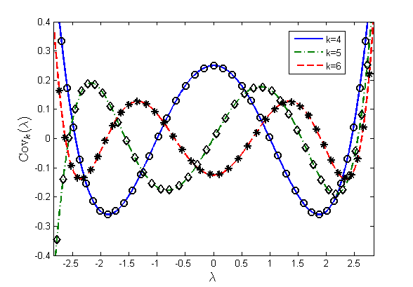
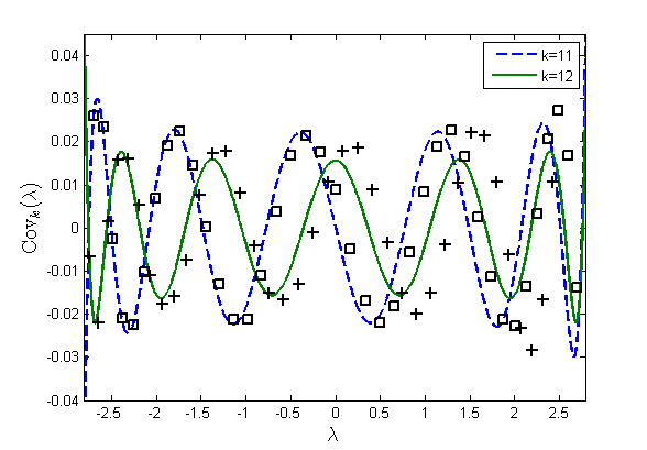
Figure 1: A comparison between $\mathop{\mathrm{Cov}}\nolimits_{k}^{tree}(\lambda)$ (marked by lines), and $\mathop{\mathrm{Cov}}\nolimits_{k}^{emp}(f,G)$, for a single realization of $G(4000,3)$ (denoted by different markers), where $\log_{d-1}(n)=11.97$.
Upper figure: a comparison for $k=4,5,6$. Lower figure: $k=11,12$.

Although for large distances, the empirical covariance deviates from $\mathop{\mathrm{Cov}}\nolimits_{k}^{tree}(\lambda)$, it seems that the expected rate of decay is reproduced quite well, so that asymptotically $|\mathop{\mathrm{Cov}}\nolimits_{k}^{emp}(f,G)|\sim(d-1)^{-k/2}$. In order to test this assumption, we introduce for a given $G(n,d)$ and $k$, the two norms

$$N_{k}^{emp}(G)=\frac{1}{n}\sqrt{\sum_{n}(\mathop{\mathrm{Cov}}\nolimits_{k}^{emp}(f^{(i)},G))^{2}}$$ (23)

$$N_{k}^{tree}(G)=\frac{1}{n}\sqrt{\sum_{n}(\mathop{\mathrm{Cov}}\nolimits_{k}^{tree}(\lambda_{i}))^{2}}$$

and define the (scaled) norm deviation as:

$$\Delta N(G,k)=\frac{N_{k}^{emp}-N_{k}^{tree}}{N_{k}^{emp}+N_{k}^{tree}}$$ (24)

If the asymptotic rate of decay of $\mathop{\mathrm{Cov}}\nolimits_{k}^{tree}$ and $\mathop{\mathrm{Cov}}\nolimits_{k}^{emp}$ is similar , then $|\Delta N|$ will be bounded away from 1 for all $k$ and $n$.
The (average) norm deviation of an eigenvector is a function of the three parameters $n,d$ and $k$. However, a comparison of the norm deviation for several realizations of $(n,d)$ graphs with various values of $n$ and $d$, suggest that it might be well approximated by a function of two parameters only - $d$, and the scaled parameter $k/\log_{d-1}(n)$ (see figure 2-left). For a fixed value of $\log_{d-1}(n)$, the deviation decreases as $d$ increases (figure 2-right). In addition, for $k/\log n\leq 1$, the norm deviation is bounded away from one, for any $d$. Since the diameter of an $(n,d)$ graph is very close to $\log(n\log n)$, we get that $\max(k)/\log n$ approaches one as $n$ approaches infinity, therefore we expect $|\Delta N|$ to be bounded away from one for all $k$.

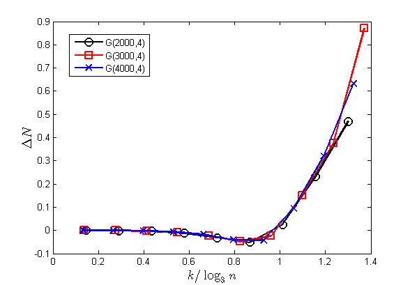
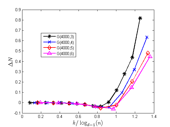
Figure 2: The scaled norm deviation (24) for several realizations of regular graphs.
Left: $\Delta N$, as a function of $k/\log_{3}(n)$, for 3 realizations of 4-regular graphs consisting of 2000,3000 and 4000 vertices.
Right: $\Delta N$, as a function of $k/\log_{d-1}(n)$, for $(4000,3),(4000,4),(4000,5)$ and $(4000,6)$ graphs.

4 The limiting distribution of eigenvectors

In the last section we have shown some of the similarities between the limiting expressions for the covariance of regular graphs and the autocorrelation of chaotic billiards $(\ref{eq:CovBerry2})$. In this section and the next, we present extensive numerical evidence, which suggest that the distribution of eigenvectors of $(n,d)$ graphs follows a Gaussian measure, resembling the conjectured distribution [10] for eigenvectors of quantum billiards (see section 2.1).
In order to examine the limiting distribution of the eigenvectors components of an $(n,d)$ graph, we have to define at first what is the ensemble we are interested in. As an example, we can fix a graph $G=(V,E)$, a vertex $v_{i}\in V$ and ask for the distribution $f^{(j)}_{i}$ of the $i$th component of a randomly chosen eigenvector. A second option is to fix an eigenvalue $\lambda_{0}\in[-2\sqrt{d-1},2\sqrt{d-1}]$, and ask for the limiting distribution of an arbitrary vertex, where we choose a graph on random, and look at the eigenvector which has the closest eigenvalue to $\lambda_{0}$. In the same manner, it is possible to fix an $(n,d)$ graph, an eigenvector $f^{(j)}$ and ask for the limiting distribution $f^{(j)}_{i}$ of a randomly chosen vertex $v_{i}\in V$.
In the following, we suggest that as $n\rightarrow\infty$, the distribution of the eigenvectors components, with respect to the first two ensembles is converging to a Gaussian. As for the third ensemble, numerical simulations (e.g. [3]), together with the results of this work imply that a limiting distribution for that ensemble may not exist.
For the sake of clarity, we begin by considering the limiting distribution of a single vertex, which will be followed by the study of a multivariate version. We will denote by $p(x)$ and $\Phi(x)$, the density and the cumulative distribution function (cdf) of the standard normal variable:

$$p(x)=\frac{1}{\sqrt{2\pi}}e^{-x^{2}/2}\quad,\quad\Phi(x)=\int_{-\infty}^{x}p(y)dy$$ (25)

4.1 The limiting univariate distribution

Based on numerical simulations we suggest the following limits:

• Hypothesis I (univariate): For asymptotically almost any $G(n,d)=(V,E)$ and $v_{i}\in V$, the probability that $f^{(j)}(v_{i})<x$, where $f^{(j)}$ is an adjacency eigenvector, chosen uniformly from $\{f^{(2)},f^{(3)},...f^{(n)}\}$, is bounded by

  $$\left|\mathbb{P}(f^{j}(v_{i})<x)-\Phi(x)\right|<\Delta(n)$$ (26)

  where $\Delta(n)\rightarrow 0$ as $n\rightarrow\infty$.

• Hypothesis II (univariate): For a given $\lambda_{0}\in[-2\sqrt{d-1},2\sqrt{d-1}]$ and $1\leq i\leq n$, the distribution of $f^{(\lambda_{0})}(v_{i})$, is converging to the normal distribution (25), where $f^{(\lambda_{0})}$ is an adjacency eigenvector with the closest eigenvalue to $\lambda_{0}$ of a uniformly randomly chosen $(n,d)$ graph.

These assumptions may be examined by comparing the appropriate empirical cumulative distribution functions to $\Phi(x)$. A plausible measure to the distance between two cumulative distributions $\mathcal{P}_{1}(x),\mathcal{P}_{2}(x)$ is the Kolmogorov-Smirnov (KS) distance:

$$\mathcal{D}^{KS}_{i}=\sup\left|\mathcal{P}_{1}(x)-\mathcal{P}_{2}(x)\right|$$ (27)

According to Kolmogorov theorem, if $\mathcal{P}_{2}(x)$ is an empirical cdf of $n$ iid variables, generated with respect to the cdf $\mathcal{P}_{1}(x)$, then the distribution of $\mathcal{D}^{KS}_{i}$ is given by

$$\lim_{n\rightarrow\infty}\mathbb{P}\left(\mathcal{D}^{KS}_{i}\leq\frac{y}{\sqrt{n}}\right)=1-2\sum_{q=1}^{\infty}(-1)^{q-1}e^{-2q^{2}y^{2}}$$ (28)

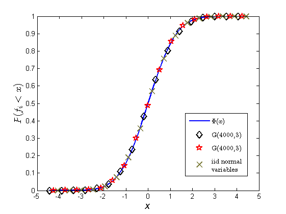
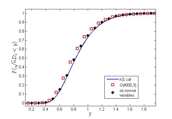
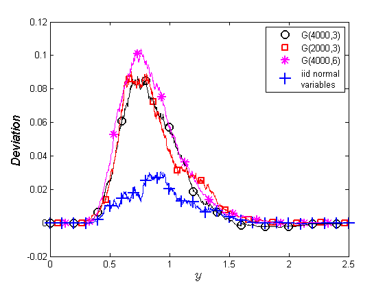
Figure 3: Upper left figure: a comparison between $\mathcal{F}_{i}(x)$ for two vertices of a realization of $(4000,3)$ graph, the empirical cdf of 4000 iid normal variables and $\Phi(x)$.
Upper right figure: a comparison between (28), the empirical cdf of $\mathcal{D}^{KS}$ for 4000 vertices of a $(4000,3)$ graph and the empirical cdf of $\mathcal{D}^{KS}$ for 4000 independent vectors of 4000 iid normal variables.
Lower figure: deviations of the empirical cdf of $\mathcal{D}^{KS}$ from (28), for a single realization of $G(4000,3)$, $G(2000,3)$ , $G(4000,6)$ and the iid normal variables. A positive deviation corresponds to a faster convergence than predicted by (28).

In order to test the first hypothesis we have generated realizations of $(n,d)$ graphs for several values of $n$ and $d$. For a given graph and a vertex $v_{i}\in V$, the empirical cdf is given by

$$\mathcal{F}_{i}(x)=\frac{1}{n}\#\{j|f^{(j)}_{i}<x\}$$ (29)

A numerical comparison between $\mathcal{F}_{i}(x)$ to $\Phi(x)$ shows persuasively that the differences between the two distributions are of order $1/\sqrt{n}$, as is demonstrated in the upper left plot in figure 3.
Since the components $f^{(j)}_{i}$ are not independent, the KS distance between $\mathcal{F}_{i}(x)$ and $\Phi(x)$ is not expected a priori to follow (28). However, the measured KS distances for different vertices of the same graph, was found to be very close to (28), as can be seen in figure 3 (upper right figure). In fact, the observed convergence of $\mathcal{D}^{KS}$ seems to be slightly faster than predicted by (28), irrespective of $n$ and $d$ (figure 3-lower figure).

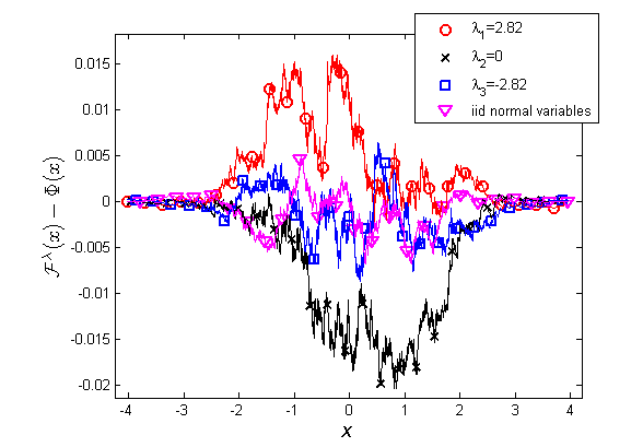
Figure 4: The deviation of the empirical cdf, calculated according to the requirements of hypothesis II, from $\Phi(x)$. The different curves correspond to $\lambda_{1}=2.82$, $\lambda_{2}=0$, $\lambda_{3}=-2.82$ and the empirical cdf of 10000 iid normal variables.

In order to examine hypothesis II, we have generated 10000 realizations of $(6000,3)$ graphs, for which the spectrum is supported on $\pm 2\sqrt{2}\approx 2.828$. We have compared $\mathcal{F}^{\lambda}(x)$ - the empirical cdf of the appropriate components, for various values of $\lambda$, varying from $-2.82$ up to $2.82$. In this case as well, the distance between $\mathcal{F}^{\lambda}(x)$ and $\Phi(x)$ tends to zero as $1/\sqrt{n}$. In addition, no substantial differences in the limiting distribution, nor in the rate of convergence were observed for different values of $\lambda$, as we demonstrate in figure 4.

4.2 The multivariate limiting distribution

In order to formulate a multivariate version of the suggested distributions, we introduce the following notation:
For a graph $G=(V,E)$, and $U=\{u_{1},...u_{m}\}\subset V$, the distance matrix $D(U,G)$ is defined as: $(D(U,G))_{ij}=|i-j|$. $\mathop{\mathrm{diam}}\nolimits(U)=\max\left(D(U,G)\right)$ is the diameter of $U$ in $G$. For a given $d$, a distance matrix is ’good’, if it can be embedded in a $d-$regular tree. A subset $U\subset V$ is good, if its distance matrix is good. We should note that if $G$ is an $(n,d)$ graph, then (due to the local tree property) almost any $U\subset V$ with $\mathop{\mathrm{diam}}\nolimits(U)<\log n/2$ is good.
For $U\subset V$ and $\lambda\in[-2\sqrt{d-1},2\sqrt{d-1}]$, we define the limiting covariance matrix $\mathcal{C}_{\lambda}(U)$ by $(\mathcal{C}_{\lambda})_{ij}=\mathop{\mathrm{Cov}}\nolimits_{D_{ij}}^{tree}(\lambda)$, where $\mathop{\mathrm{Cov}}\nolimits_{k}^{tree}(\lambda)$ is given by (20).
We will denote by $p(\mathbf{x},\Sigma)$ and $\Phi(\mathbf{x},\Sigma)$, the density and the cdf of the multinormal variable $\mathbf{x}=(x_{1},...x_{m})^{T}$ with mean zero and covariance matrix $\Sigma$:

$$p(\mathbf{x},\Sigma)=\frac{1}{\sqrt{(2\pi)^{m}|\Sigma|}}e^{-\langle\mathbf{x},\Sigma^{-1}\mathbf{x}\rangle/2}\quad,\quad\Phi(\mathbf{x},\Sigma)=\int_{-\infty}^{\mathbf{x}}p(\mathbf{y},\Sigma)d\mathbf{y}$$ (30)

Equipped with this notation, we suggest the following for $\lambda_{0}\in[-2\sqrt{d-1},2\sqrt{d-1}]$ and a fixed $m$:

• Hypothesis I(multivariate): For almost any $G(n,d)=(V,E)$ and a good $U\subset V$ of small diameter in $G$, the probability that $f(U)=(f(u_{1}),...f(u_{m}))^{T}<\mathbf{x}$, where $f$ is an adjacency eigenvector, chosen uniformly from the spectral window $[\lambda_{0},\lambda_{0}+\epsilon]$, is bounded by

  $$\left|\mathbb{P}(f(U)<\mathbf{x})-\Phi(\mathbf{x},\mathcal{C}_{\lambda_{0}})\right|<\Delta(n,\epsilon)$$ (31)

  where $\Delta(n,\epsilon)\rightarrow 0$ as $\epsilon\rightarrow 0$ but $\epsilon n\rightarrow\infty$.

• Hypothesis II (multivariate): For a good distance matrix $D$, the distribution of $f^{(\lambda_{0})}(U)$ converges as $n\rightarrow\infty$, to the multinormal distribution (30) with covariance matrix $\mathcal{C}_{\lambda_{0}}$, where $f^{(\lambda_{0})}$ is an adjacency eigenvector with the closest eigenvalue to $\lambda_{0}$ of a uniformly chosen $(n,d)$ graph and $U$ satisfies $D_{G}(U)=D$.

Two remarks are in order. First, in hypothesis I we avoid the question how small should $\mathop{\mathrm{diam}}\nolimits(U)$ be, as we base the hypothesis mainly on numerical simulations, which are applicable for small-diameter distance matrices only (see section 5.2). Second, we should note that in equation (30) we assume the existence of the inverse covariance matrix. The existence of an inverse for $\mathcal{C}_{\lambda_{0}}$ will be discussed in the next section, where we show that for distance matrices which contain a vertex and all of its neighbors, the covariance is singular. We also demonstrate how this calculative obstacle can be removed by a simple coordinate transformation.
Unlike the univariate conjectures, a comprehensive numerical examination of the multivariate versions is a hard task. As a beginning, we had to make do with the comparison of the empirical cdf of two adjacent vertices to (31), where for this configuration $\mathcal{C}_{\lambda}$ is given by $(\mathcal{C}_{\lambda})_{11}=(\mathcal{C}_{\lambda})_{22}=1,(\mathcal{C}_{\lambda})_{12}=(\mathcal{C}_{\lambda})_{21}=\lambda/d$.
For $k$ iid bivariate normal variables with mean zero and covariance $\mathcal{C}_{\lambda}$, the empirical cdf is expected to converge to $\Phi(\mathbf{x},\mathcal{C}_{\lambda})$ as $1/\sqrt{k}$. In order to check the second hypothesis we have measured the value of two adjacent vertices $(f^{(j)}_{1},f^{(j)}_{2})$ over 20000 realizations of $(6000,4)$ graphs from the eigenvector with the closest eigenvalue to some $\lambda$. In order to evaluate the rate of convergence as a function of the number of realizations, we have calculated for various values of $k$, the empirical cdf for the first $k$ measurements:

$$\mathcal{F}_{\lambda}^{k}(\mathbf{x})=\frac{1}{k}\{\#i|i\leq k,f^{(j)}_{1}<x_{1},f^{(j)}_{2}<x_{2}\}$$ (32)

Finally, for every $lambda$ and $k$, we have calculated $\max\left|\Phi(\mathbf{x},\mathcal{C}_{\lambda})-\mathcal{F}_{\lambda}^{k}(\mathbf{x})\right|$. As demonstrated in figure 5 the deviation does decrease as $k$ increases, however the convergence is slower than the one measured for iid bivariate normal variables. In addition, for larger eigenvalues (smaller Laplacian eigenvalues), we have observed a faster convergence.

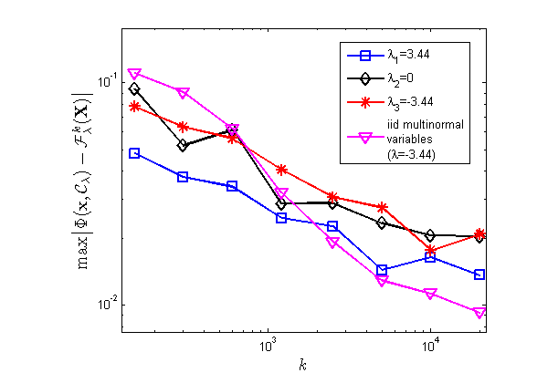
Figure 5: The maximal deviation between the cumulative distributions $\mathcal{F}_{\lambda}^{k}(\mathbf{x})$ and $\Phi(\mathbf{x},\mathcal{C}_{\lambda})$ as a function of $k$ - the number of generated graphs (logarithmic scale). The different curves correspond to $\lambda_{1}=3.44$, $\lambda_{2}=0$ and $\lambda_{3}=-3.44$. The maximal deviation is compared to that of $k$ iid vectors, generated with respect to the measure $\Phi(\mathbf{x},\mathcal{C}_{-3.44})$.

The first hypothesis is harder to test directly, as it requires the generating (and more problematic, the diagonalization) of a very large graph, in order to have a narrow spectral window which contains many eigenvectors. By using MATLAB’s function eigs.m We have explored relatively narrow spectral windows ($\lambda_{max}-\lambda_{min}\approx 0.1$) of $(13000,3)$ graphs, which contains between 200 to 400 eigenvectors (the exact number depends on the spectral density at $\lambda$). The KS distance between the empirical cdf for those windows and $\Phi(\mathbf{x},\mathcal{C}_{\lambda})$, was consistent with the measured deviation in the previous experiment for the same number of samples.
An additional support to the Gaussian approximation will be introduced in the next section, where we reconstruct the structure of the nodal pattern of an eigenvector, assuming the suggested normal distribution.

5 The nodal structure of eigenvectors

For a graph $G=(V,E)$ and a function $f(V)$, we define the induced nodal graph $\tilde{G}_{f}=(V,\tilde{E}_{f})$ , by the deletion of edges, which connect vertices of opposite signs in $f$: $\tilde{E}_{f}=\{(v_{i},v_{j})\in E|f_{i}f_{j}>0\}$. In this section we analyze the nodal pattern of the eigenfunctions, assuming the multinormal distribution, as stated in hypothesis II. We will demonstrate that this assumption allows us not only to evaluate the expectation of the nodal count, but also to estimate the distribution of the size and shape of domains. In particular we will demonstrate that the nodal structure cannot be imitated by percolation-like models.

5.1 Distribution of valency

We begin by calculating $p_{e}(\lambda)$ - the probability of an edge $e\in E$ of a random graph, to belong to $\tilde{E}_{f}$ for an eigenvector $f$ with eigenvalue $\lambda$. This is twice the probability of two adjacent vertices to be positive, which according to hypothesis II, equals

$$p_{e}(\lambda)=2\int_{0}^{\infty}\int_{0}^{\infty}d\mathbf{f}\frac{1}{2\pi\sqrt{|\mathcal{C}_{\lambda}|}}\exp\left(-\frac{1}{2}\langle\mathbf{f},\mathcal{C}_{\lambda}^{-1}\mathbf{f}\rangle\right)$$ (33)

where $(\mathcal{C}_{\lambda})_{11}=(\mathcal{C}_{\lambda})_{22}=1$ , $(\mathcal{C}_{\lambda})_{12}=(\mathcal{C}_{\lambda})_{21}=\lambda/d$. Integrating, we get that:

$$p_{e}(\lambda)=\frac{1}{2}+\frac{1}{\pi}\arcsin\left(\frac{\lambda}{d}\right)$$ (34)

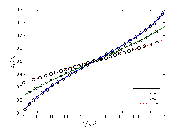
Figure 6: A comparison between the Gaussian prediction for $p_{e}(\lambda)$ (lines) and the empirical result (markers) for a single random realization of 3,6 and 15 regular graphs on 4000 vertices.

$p_{e}(\lambda)$ is symmetric with respect to $\lambda=0$. In addition, since $|\lambda|\leq 2\sqrt{d-1}$, for small values of $d$, $p_{e}(\lambda)$ varies considerably along the spectrum (thus, for $d=3$, $p_{e}(\lambda)$ can take values in the interval $[0.1,0.9]$), while for large $d$ the changes are moderate (for $d=100$ for example, it is constrained to $[0.44,0.56]$). As demonstrated in figure 6, this result describes with high accuracy the observed probability, for various values of $d$.
The Gaussian model predicts as well a distribution for the valency of vertices in $\tilde{G}_{f}$. In order to evaluate $p_{j}(\lambda)$ - the probability of a vertex $v_{0}\in V$ to be of valency $j$ in $\tilde{G}_{f}$, one should consider the mutual distribution of $f_{0}$ and its $d$ neighbors $\{f_{1},...f_{d}\}$. The appropriate covariance entries are given by $(\mathcal{C}_{\lambda})_{ii}=1,(\mathcal{C}_{\lambda})_{0j}=(\mathcal{C}_{\lambda})_{j0}=\lambda/d$ and $(\mathcal{C}_{\lambda})_{jk}=(\lambda^{2}-d)/d(d-1)$, for $0\leq i\leq d$ ,$1\leq j,k\leq d$ and $j\neq k$.
This matrix is singular, as $(\lambda,-1,-1,...-1)^{T}$ is an eigenvector of $\mathcal{C}_{\lambda}$ with zero eigenvalue. This singularity is due to the constraint $\lambda f_{0}=\sum_{j}f_{j}$ which is kept by the Gaussian model. In order to avoid the singularity we may integrate with respect to the new Gaussian variables $\tilde{\mathbf{f}}=(\lambda f_{0}-\sum_{j}f_{j},f_{1},...f_{d})^{T}$. Introducing the (invertible) matrix $\tilde{\mathcal{C}}_{\lambda}$, obtained from $\mathcal{C}_{\lambda}$ by changing the of diagonal terms in the zeroth row and column to zero, $p_{j}(\lambda)$ can be written as:

$$p_{j}(\lambda)=2{d\choose j}\int\frac{d\tilde{\mathbf{f}}}{\sqrt{(2\pi)^{d}|\tilde{\mathcal{C}}_{\lambda}|}}\delta(\tilde{f}_{0})\theta(f_{0})\prod_{i=1}^{j}\theta(f_{i})\prod_{l=j+1}^{d}\theta(f_{l})\exp[-\frac{1}{2}\langle\tilde{\mathbf{f}},\tilde{\mathcal{C}}_{\lambda}^{-1}\tilde{\mathbf{f}}\rangle]$$ (35)

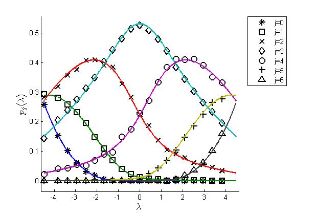
Figure 7: A comparison between the Gaussian prediction of $p_{j}(\lambda)$ and the empirical result for a single realization of $G(4000,6)$.

where the prefactor is due to the sign symmetry and the different alternatives to choose $j$ out of $d$ adjacent vertices. An immediate result of this expression is the symmetry $p_{j}(\lambda)=p_{d-j}(-\lambda)$. This integral cannot be calculated explicitly, however it can be evaluated, e.g. by the method of [30]. As in the study of $p_{e}(\lambda)$ the Gaussian prediction is very close to the observed results. As an example, in figure 7 we compare the Gaussian prediction for $p_{j}(\lambda)$ and $d=6$, evaluated by the function qscmvnv.m [31], to the measured result for a single realization of a $(4000,6)$ graph.

5.2 The nodal count of an eigenfunction

In [1], the following intriguing properties of the nodal count $\{\nu_{j}\}_{j=1}^{n}$ for the eigenvectors of $(n,d)$ graphs were observed. First, for all $j<j_{0}(d,n)$, $\nu_{j}$ was found to be exactly $2$, where the relative part $j_{0}/n$ of eigenvectors with exactly two nodal domains is increasing with $d$. Second, for small values of $d$, and for $j>j_{0}$, the nodal count increases approximately linearly with $j$. While the known bounds on the nodal count (see section 2.2) are far from being satisfactory in explaining this behavior, we would like to demonstrate in this section, how does the expected nodal count emerges from the Gaussian model.
Adopting the Gaussian expression (34) for $p_{e}(\lambda)$, it is possible to derive a lower bound on the expected nodal count of an eigenvector. The number $N$ of connected components of a graph $G=(V,E)$, is given by $N=V-E+C$, where $C$ is the number of independent cycles in $G$. Since on average, the induced nodal graph $\tilde{G}_{f}$ posses $p_{e}(\lambda)\cdot|E|=\frac{nd}{2}p_{e}(\lambda)$ edges and $n$ vertices, the expected nodal count is bounded from below (for all of the eigenvectors but the first) by

$$E\left(\nu(n,\lambda)\right)\geq\max\left\{2,n\left(1-\frac{d}{2}p_{e}(\lambda)\right)\right\}$$ (36)

We should note that this bound is effective only for $d\leq 7$, as for larger values, $1-dp_{e}(\lambda)/2$ is negative for $|\lambda|\leq 2\sqrt{d-1}$.
For low values of $d$ this crude bound matches surprisingly well the observed nodal count, as is demonstrated in figure 8 for a $(4000,3)$ graph.

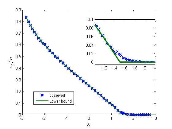
Figure 8: A comparison between (36) and the observed count for a single realization of $G(4000,3)$. The inset is a magnification of the spectral window near the bound’s flexion - the only part of the spectrum in which the observed count deviates considerably from the bound.

The good agreement can be understood if we consider the critical properties of the nodal pattern. Numerical observations [32] suggest that for $d\leq 5$, the induced nodal graph $\tilde{G}_{f}$ exhibits a phase transition at some $\lambda_{c}$ as $n\rightarrow\infty$. In the subcritical phase ($\lambda<\lambda_{c}$), the size of the largest nodal domains is proportional to $\log n$, while in the supercritical phase ($\lambda>\lambda_{c}$), two giant components of order $n$ emerge.
As the number of connected components of size $\log n$ in an $(n,d)$ graph, which contain $\log(\log n)$ cycles is almost surely zero, the expected number of independent closed cycles in $\tilde{G}_{f}$ in the subcritical regime must be much smaller than $n\log(\log n)/\log n$ (as there cannot be more than $n/\log n$ domains comparable in size to $\log n$). As a result, for $\lambda<\lambda_{c}$ the deviation between (36) to the expected count is at most of order $1/\log(n)$. This result is reflected in figure 9, which demonstrate that for $d\leq 5$ (where a subcritical phase is observed), the measured count converges to (36), for low enough eigenvalues.

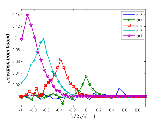
Figure 9: The deviation of $\nu_{\lambda}/n$ from the lower bound (36), for 3,4,5,6 and 7 regular graphs on 4000 vertices.

The fact that only two nodal domains are observed for a large number of eigenvectors is also consistent with the existence of a supercritical phase. A general property of supercritical systems is the scarcity of large but finite clusters. the expected number of clusters of size $s$ decays asymptotically as $\exp(-s(p-p_{c})^{\gamma})$, for some (model dependent) positive $\gamma$. Therefore, the supercritical phase consists of a giant component and ’dust’. When we consider the nodal pattern of supercritical eigenfunction (i.e. those with $\lambda>\lambda_{c}$) two special phenomena occur. The first is the appearance of two giant components - a positive and a negative domains. The second is the rarity of small domains: as was mentioned in section 2.2, the distribution of the eigenvectors is constrained, preventing the existence of small domains for large enough values of $\lambda$. As a result, we expect to find only rarely more than 2 nodal domains, for a considerable amount of first eigenvectors (which are deep enough in the supercritical regime). Moreover, as $d$ increases, the value of $\lambda_{c}$ decreases, therefore the expected number of such eigenvectors is supposed to increase with $d$ (as is indeed observed).
As the size distribution of clusters is expected to decay rapidly, we can tighten the bound on the expected nodal count considerably, by calculating $\nu_{k}(n,\lambda)$ - the expected number of domains of size $k$ for small values of $k$. It is easy to see that $\nu_{1}(n,\lambda)=np_{0}(\lambda)$ where $p_{0}(\lambda)$ is given by (35). For $k>1$ the calculation can be carried out in the same spirit: The probability for $k$ given vertices to form a nodal domain of size $k$ can be evaluated, through a $(k(d-1)+2)$ dimensional integral (over the $k$ vertices and their $k(d-2)+2$ neighbors), in a similar manner to (35). Finally, $\nu_{k}(n,\lambda)$ is given (up to small corrections) by summing the probabilities over all trees of size $k$ and maximal valency $d$, multiplied by the number of such trees in $G$. The agreement between the Gaussian prediction to the observed distribution of $\nu_{k}$ is demonstrated in figure 10.

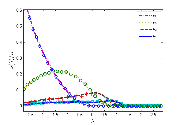
Figure 10: The Gaussian prediction for $\nu_{k}/n$ for $d=3$ and $1\leq k\leq 40$ (lines), compared to the observed count (markers) for a single realization of $G(4000,3)$.

As $E(\nu)=\sum_{k=1}^{\infty}\nu_{k}$, we get that $\sum_{i=1}^{k}\nu_{k}(n,\lambda)$ should converge to $E(\nu(\lambda,n))$. In figure 11 we plot the maximal deviation between $\sum\nu_{k}$ (for $1\leq k\leq 4$) and the measured count of $(4000,d)$ graphs for $3\leq d\leq 10$. It can be seen that the converges is much faster for $d>5$. This is consistent with relatively slow decay in the size distribution, which is expected in the vicinity of the critical point.

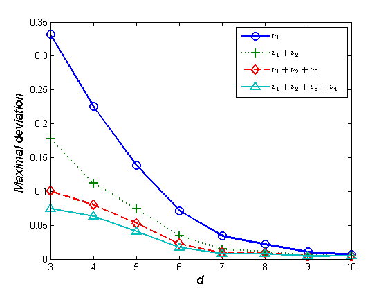
Figure 11: The maximal deviation between the measured nodal count of $3\leq d\leq 10$ regular graphs on 4000 vertices to the expected number of domains, smaller or equal than 1,2,3 and 4 vertices.

5.3 Eigenvectors and percolation

For a $G(n,d)$ graph and $0\leq p\leq 1$, the induced percolation graph $G(n,d,p)$ is obtained by deleting the edges of $G$ independently with probability $1-p$. As was mentioned in section 2.1, for two-dimensional billiards, it is believed that the nodal pattern exhibits (in the semi-classical limit) a percolation-like behavior [2]. In this section we compare the properties of $G(n,d,p)$ to the nodal pattern of an eigenvector, satisfying $p_{e}(\lambda)=p$ (see eq. 34).
An important difference between the two models is their valency distribution. For percolation, as the deletion of different edges is independent, the probability of a vertex in $G(n,d,p)$ to be of valency $j$ is given by

$$p_{j}^{perc}(p)={d\choose l}p^{l}(1-p)^{d-l}$$ (37)

which is essentially different from $p_{j}(\lambda)$ (35) - the equivalent expression for the nodal pattern. As will be demonstrated soon, by changing the valency distribution, we change global properties of the pattern as well.
The differences between the two processes are not limited to local measures such as $p_{j}$, but also for events which involve several vertices. For example, the probability to have a connected cluster of size $k$ in $G(n,d,p)$ is positive for any $p>0$, and can be expressed through $p_{j}^{perc}(p)$. As for the nodal pattern, for any $k\in\mathbb{N}$ there is some $\lambda_{max}$, so that for $\lambda>\lambda_{max}$ the probability to have a domain smaller than $k$ is zero. In addition, as was demonstrated above, the quantities $\nu_{k}$ cannot be reduced to simple functions of $p_{j}(\lambda)$.
Finally, we would like to show that the critical threshold for the two models is different. In [33] the critical probability for $G(n,d,p)$ was found to be $p_{c}=1/(d-1)$. It is not hard to verify that for the nodal pattern $p_{e}(\lambda_{c})>1/(d-1)$. Consider for example the case $d=3$, where $p_{c}=1/2=p_{e}(\lambda=0)$. As was mentioned before, for $\lambda=0$ there are no interior points in the nodal domains, therefore, for $d=3$ all nodal domains must be linear chains. however, percolation on linear chains is always subcritical, therefore necessarily $\lambda_{c}>0$. By similar arguments, this will also be the case for $d>3$.
We would like to note that the mismatch between the properties of the Laplacian nodal pattern and $G(n,d,p)$ should not come as a great surprise. One of the main arguments in favor of the percolation model [17] for 2 dimensional billiards, is that the asymptotic rate of decay of the eigenvectors’ covariance (4) is fast enough in order to neglect correlations, according to the so called ’Harris criterion’ [34]. However, the covariance for eigenvectors of $(n,d)$ graphs (20), does not fulfill the requirements of this criterion, implying that the scaling limit of the two models will differ. We should note that the requirements of this criterion are not fulfilled for billiards in more than two dimensions as well. This suggest that the resemblance between the nodal pattern of Laplacian eigenvectors to percolation is a two dimensional phenomenon.

6 Conclusions

As a summary, we collect the main new results of this work concerning the structure of Laplacian (Adjacency) eigenvectors:

1. In the limit $n\rightarrow\infty$, the empirical covariance (12) of an eigenvector of a uniformly chosen $(n,d)$ graph, for a distance $k<log_{d-1}(n)/2$ is given by

   $$\quad\mathop{\mathrm{Cov}}\nolimits_{k}^{tree}(\lambda)=\frac{1}{d(d-1)^{k/2}}\left((d-1)U_{k}\left(\frac{\lambda}{2\sqrt{d-1}}\right)-U_{k-2}\left(\frac{\lambda}{2\sqrt{d-1}}\right)\right)$$ (38)

   which decays exponentially with $k$. For $k>\log_{d-1}(n)/2$, this approximation loses its accuracy. however, the observed rate of decay is still exponential in $k$.

2. We provide numerical evidence in support of the hypothesis that the distribution of the adjacency (or Laplacian) eigenvectors follows the Gaussian measure

   $$p(f(U))=\frac{1}{\sqrt{(2\pi)^{m}|\mathcal{C}_{\lambda_{0}}|}}\exp\left[-\frac{1}{2}\langle f(U),\mathcal{C}_{\lambda_{0}}^{-1}f(U)\rangle\right]$$ (39)

   For any $\lambda_{0}\in[-2\sqrt{d-1},2\sqrt{d-1}]$.

3. We used the Gaussian measure to predict the expected number of nodal domains in an eigenfunction and its dependence in the eigenvalue. We have shown the consistency of the Gaussian hypothesis with various nodal properties, such as valency and size distribution.

4. We have shown that the nodal structure of the Laplacian eigenvectors differ from the cluster structure of $G(n,d,p)$. The two models are not sharing the same critical point, and the structure of a typical components does not follow the same law in the two cases.

References

- [1] Lee J Dekel Y and Linial N. chapter Eigenvectors of Random Graphs: Nodal Domains, pages 436–448. 2007. 10.1007/978-3-540-74208-1_32.
- [2] Bogomolny E and Schmit C. Percolation Model for Nodal Domains of Chaotic Wave Functions. Physical Review Letters, 88(11):114102, March 2002.
- [3] Linial N Hoory S and Wigderson A. Expander graphs and their applications. Bull. Amer. Math. Soc. (N.S.), 43(4):439–561 (electronic), 2006.
- [4] Shi J and Malik J. Normalized cuts and image segmentation. IEEE Transactions on Pattern Analysis and Machine Intelligence, 22(8):888–905, 2000.
- [5] Coifman R R. Perspectives and challenges to harmonic analysis and geometry in high dimensions: geometric diffusions as a tool for harmonic analysis and structure definition of data. In Perspectives in analysis, volume 27 of Math. Phys. Stud., pages 27–35. Springer, Berlin, 2005.
- [6] Simon H D Pothen A and Liou K P. Partitioning sparse matrices with eigenvectors of graphs. SIAM J. Matrix Anal. Appl., 11(3):430–452, 1990. Sparse matrices (Gleneden Beach, OR, 1989).
- [7] Lovász L. Random walks on graphs: a survey. In Combinatorics, Paul Erdős is eighty, Vol. 2 (Keszthely, 1993), volume 2 of Bolyai Soc. Math. Stud., pages 353–397. János Bolyai Math. Soc., Budapest, 1996.
- [8] Rivin I Jakobson D, Miller S D and Rudnick Z. Eigenvalue spacings for regular graphs. ArXiv High Energy Physics - Theory e-prints, September 2003.
- [9] Smilansky U. Quantum chaos on discrete graphs. Journal of Physics A: Mathematical and Theoretical, 40(27):F621–F630, 2007.
- [10] Berry M V. Regular and irregular semiclassical wave functions. Journal of Physics A Mathematical General, 10:2083–2091, 1977.
- [11] Urbina J D and Richter K. Semiclassical construction of random wave functions for confined systems. Physical Review E, 70(1):015201–+, July 2004.
- [12] Gnutzmann S Blum G and Smilansky U. Nodal domains statistics: A criterion for quantum chaos. Physical Review Letters, 88(11):114101, March 2002.
- [13] Joas C Elon Y, Gnutzmann S and Smilansky U. Geometric characterization of nodal domains: the area-to-perimeter ratio. J. Phys. A, 40(11):2689–2707, 2007.
- [14] Courant R and Hilbert D. Methods of mathematical physics. Vol. I. Interscience Publishers, Inc., New York, N.Y., 1953.
- [15] Gnutzmann S Foltin, G and Smilansky U. The morphology of nodal lines random waves versus percolation. Journal of Physics A Mathematical General, 37:11363–11371, November 2004.
- [16] Aronovitch A and Smilansky U. The statistics of the points where nodal lines intersect a reference curve. Journal of Physics A Mathematical General, 40:9743–9770, August 2007.
- [17] Bogomolny E and Schmit C. Random wavefunctions and percolation. Journal of Physics A Mathematical General, 40:14033–14043, November 2007.
- [18] Dubertrand R Bogomolny E and Schmit C. SLE description of the nodal lines of random wave functions. ArXiv Nonlinear Sciences e-prints, September 2006.
- [19] Marklof J Keating J P and Williams I G. Nodal domain statistics for quantum maps, percolation, and stochastic loewner evolution. Physical Review Letters, 97(3):034101, 2006.
- [20] Bollobás B. A probabilistic proof of an asymptotic formula for the number of labelled regular graphs. European J. Combin., 1(4):311–316, 1980.
- [21] Bollobás B and De la Vega W F. The diameter of random regular graphs. Combinatorica, 2(2):125–134, June 1982.
- [22] McKay B D. The expected eigenvalue distribution of a large regular graph. Linear Algebra Appl., 40:203–216, 1981.
- [23] Leydold J Davies E B, Gladwell G M L and Stadler P F. Discrete nodal domain theorems. Linear Algebra Appl., 336:51–60, 2001.
- [24] Oren I Band R and Smilansky U. Nodal domains on graphs - how to count them and why?, 2007.
- [25] Bıyıkoğlu T and Leydold J. Faber-Krahn type inequalities for trees. J. Combin. Theory Ser. B, 97(2):159–174, 2007.
- [26] Leydold J Bıyıkoğlu T and Stadler P F. Laplacian eigenvectors of graphs, volume 1915 of Lecture Notes in Mathematics. Springer, Berlin, 2007. Perron-Frobenius and Faber-Krahn type theorems.
- [27] Lubetzky E Alon N, Benjamini I and Sodin S. Non-backtracking random walks mix faster, 2006.
- [28] Abramowitz M and Stegun I A. Handbook of Mathematical Functions with Formulas, Graphs, and Mathematical Tables. Dover, New York, ninth dover printing, tenth gpo printing edition, 1964.
- [29] Steger A and Wormald N C. Generating random regular graphs quickly. Combin. Probab. Comput., 8(4):377–396, 1999. Random graphs and combinatorial structures (Oberwolfach, 1997).
- [30] Genz A. Numerical computation of multivariate normal probabilities. J. Comput. Graph. Statist., 1:141–150, 1992.
- [31] Genz A. http://www.math.wsu.edu/faculty/genz/homepage.
- [32] Y Elon and U Smilansky. Level sets of eigenfunctions on regular graphs. In preparation.
- [33] Benjamini I Alon, N and Stacey A. Percolation on finite graphs and isoperimetric inequalities. Ann. Probab., 32(3A):1727–1745, 2004.
- [34] Harris A B. Effect of random defects on the critical behaviour of ising models. Journal of Physics C: Solid State Physics, 7(9):1671–1692, 1974.