Topological Disorder in Spin Models on Hierarchical Lattices.

Abstract

A general approach for the description of spin systems on hierarchial lattices with coordination number $q$ as a dynamical variable is proposed. The ferromagnetic Ising model on the Bethe lattice was studied as a simple example demonstrating our method. The annealed and partly annealed versions of disorder concerned with the lattice coordination number are invented and discussed. Recurrent relations are obtained for the evaluation of magnetization. The magnetization is calculated for the particular disorder choices, $q=2,3$ and $q=3,4$. A nontrivial localization of critical point is revealed.

I Introduction

The hierarchical models in statistical physics can be used to exactly describe the critical phenomena. For these purposes only approximate or numerical methods exist in most statistical mechanical models. Therefore complicated models representing nontrivial critical behavior and demonstrating analytical solution may be recognized as very important. A good example of such systems are spin models on hierarchical lattices. Besides the general interest related to the critical phenomena, spin models on hierarchical lattices are also formulated for description of the concrete physical systems. The interesting applications are Bethe approximation in polymer physics, and many others Pretti -esk .

The main purpose of this work is a study of spin models on hierarchical lattices with so called topological disorder. The problem of disorder for the hierarchical models is known and has been discussed in series of works dis1 -dis4 . However, disorders concerned with couplings and magnetic fields are considered mainly. So called topological disorder, describing by the changing lattice coordination number, is investigated less. In our definition topological disorder represents non-homogeneity of the lattice structure and may be even non-connected to the spins dynamics. A more precise definition of the topological disorder in context of the hierarchical models is given below within a concrete example.

Although all results in our article are related to the physics and have direct meaning in a physical sense, it is interesting to discuss their possible applications in the context of social dynamics. As is known, in the recent decades there is a rapidly growing interest to the application of the statistical physics to interdisciplinary fields (as biology, computer science, social dynamics and e.t.c). Considering the social dynamics we deal not with physical particles but with humans or crowds. The human behavior is not rather well understood and depends on many hidden factors. Nevertheless, one may suppose that in the statistical limit the new statistical laws would be obtained, which are less dependent on the individuals. As it was shown in recent decade, this conjecture is correct. The transitions from disorder to order are discovered describing the social dynamics from the statistical physics point of view. We may bring as the examples of those transitions spontaneous formation of a common language, culture or the emergence of consensus about a specific issue soc . There are also examples of scaling and universality.

As an illustration of our approach to spin systems on hierarchical lattices with changing coordination number $q$ we consider ferromagnetic Ising model on the Bethe lattice as a simplest possible example.

The article is organized as follows. In section II a simple ferromagnetic Ising model with topological disorder on hierarchical lattice is formulated. A more precise and clear definition of the topological disorder in context of the hierarchical lattices is given. The connection between proposed model and description of social dynamics is discussed in detail.

In section III annealed and partly annealed topological disorders are defined. A general method for those mathematical description is proposed. The annealed version of the topological disorder is studied for the particular realizations of the lattice structure. The critical temperature is found and analyzed.

Partly annealed and quenched topological disorders are described within ferromagnetic Ising model in section IV. The same particular realizations of the topological disorder as for the annealed one are discussed. The critical point is obtained.

Main observations are presented in conclusion.

II Ising Model on Bethe Lattice with topological disorder

The one of the simplest recursive lattices is a Cayley tree. Constructing Cayley tree one starts with a central site O. After that we connect the central site O by links with $q$ new other sites. This procedure of $q$ new sites connection by links to the each site originated on the previous step repeats $n$ times. Following this procedure one gets the recursive connected graph, containing no cycles and called the Cayley tree with coordination number $q$ and $n$ generations.

The Bethe lattice may be considered as the interior of the Cayley tree. Only sites lying deep inside Cayley tree constitute the Bethe lattice. Dealing with the Bethe lattice we suppose the respective Cayley tree is large enough to achieve thermodynamical limit and neglect boundary effects. The general structure and topology of the Bethe lattice is the same as for Calyley tree. Here we consider changing along the lattice coordination number $q_{i}$, which is different in general for the different $i$ sites, even from the same generation. The Betthe lattice is not uniform now and topological disorder related to it can be discussed.

The Hamiltonian of the Ising model on Bethe lattice reads

$$H=-J\sum_{i,j}s_{i}s_{j}-h\sum_{i}s_{i},$$ (1)

where $J$ and $h$ do not depend on the indexes $i,j$, for the sake of simplicity. The summation is over all neighbor $s_{i}$ and $s_{j}$ spins along the lattice and spin variables are $s_{i}=\pm 1$. The interpretation of this model in context of social dynamics is following. The common task of social dynamics is the understanding of the transition from an initial disordered state to a configuration that displays order. The one approach is an analogy to physics of the Ising model for ferromagnetic. The Ising model may be considered as the simplest description of the opinion dynamics. Each spin on the Bethe lattice represents a human opinion on some subject (agree/disagree units)locating in corresponding lattice site. We describe the situation in the simplest sense. The coupling $J$ is positive reflecting the fact that the people communicating with each other long or even not a very long time usually tend to have the same opinion. In other words, humans or other social units like communicate with people (social units) having usually a good agreement with them. However, it is not always true. The discussion of the anti-ferromagnetic $J$ is also meaningful. The Bethe lattice in our interpretation is not a spatial distribution of humans but a construction in relation space and represents possible ”stable” communications (relations) between ”humans” $s_{i}$. Our proposition is to consider ”humans” $s_{i}$ communicating with (acting on) some finite number of neighbors in relation space. This number, which coincides with the coordination number of lattice $q_{i}$, may be influenced by some external noise and changes in time in general. Here we consider $q_{i}$ individually for the each site $i$ and the coordination number is not the same for the all sites of the same step of the lattice generation.

An external magnetic field may be treated as an external informational factor, like TV or something similar. As we use methods of the statistical physics, the temperature is introduced and represents the noise in human opinion ( measure of uncertainty in taking stable decision ). The main weakness of the model is an absence of the small cycles (loops) in relation space. Some effects induced by relation loops may be demonstrated on more complicated hierarchical lattices (as Husimi lattice).

III Annealed topological disorder

First of all let us recall some general aspects related to the spin systems with disorder. Let the Hamiltonian may be written as $H[J,s]$, where $J$ represents disorder degree of freedom and $s$ describes the spin variables correspondingly. Suppose that the spin and disorder degrees of freedom are not thermally equilibrated and disorder degrees of freedom have their own temperature $\overline{T}$. The partition function reads:

Z $$=\int DJP(J)\exp(-\overline{\beta}F(J))$$ (2)

$$= \int DJP(J)\exp(\frac{\overline{\beta}}{\beta}\ln Z(J))$$

$$= \int DJP(J)(Z(J))^{n},$$

where $Z(J)$ and $F(J)$ are respectively partition function and free energy with given disorder $J$. Here we propose to describe the disorder by the probability distribution $P[J]$. We may consider the number $n=\frac{\overline{T}}{T}$ as a number of replicas within the replica formalism Dotsenko . The total free energy would be

$$\textbf{F}=-\frac{T}{n}\ln(<Z(J)^{n}>_{dis}),$$ (3)

where the average over. Using F one would obtain the free energy describing quenched disorder after taking the limit $n\rightarrow 0$. The $n=1$ value corresponds to annealed disorder, when both temperatures $T$, $\overline{T}$ are equal. The value $1>n>0$ may be treated here as a ”degree of quenchness”. The same heuristics arises from the non-equilibrium two temperature system viewpoint in Allahv .

Now let us consider topological disorder given by the set of $\{q_{i}\}$ variables. We describe only the case of slow changing $q_{i}$ compared with the rate of the spin flips. This assumption is in agreement with the ferromagnetic hypothesis of social opinion dynamics. It is natural to suppose that the stable relations dispose to agreement between neighbors to a greater extent. So we do not analyze a more fast rate of $q_{i}$ than it is for the annealed disorder. Also we propose the ability of the probability factorization $P(\{q_{0},...,q_{M}\})=P(q_{0})...P(q_{M})$.

The one of the best methods developed for the models on hierarchical lattices is a so-called dynamical approach din0 -Monroe . Here we propose to modify this formalism for our purposes. The main quantity to be calculated is $<Z(\{q_{i}\})^{n}>_{dis}$. Let us start from the description of the annealed topological disorder $n=1$. The main advantage of the dynamical approach is that for the models formulated on recursive trees the exact recursion relations can be derived. When the tree is cut apart at the central site $O$, it separates into $q_{0}$ identical branches. According to it for the Hamiltonian (1) one can write

$$\textbf{Z}=<Z(\{q_{i}\})>_{dis}=\sum_{q_{0}}P(q_{0})\sum_{s_{0}}\exp(\beta hs_{0})\times$$

$$<g_{k}^{(1)}(q_{0},s_{0})...g_{k}^{(q_{0})}(q_{0},s_{0})>_{dis},$$ (4)

where independent replicas $g_{k}^{(i)}(q_{0},s_{0})$ are invented. The Eq. (4) also may be rewritten as

$$<Z(\{q_{i}\})>_{dis}=\sum_{q_{0}}P(q_{0})\sum_{s_{0}}\exp(\beta hs_{0})\times$$

$$<g_{k}(s_{0})>_{dis}^{q_{0}},$$ (5)

where

$$<g_{k}(s_{0})>_{dis}=\sum_{q_{0}}P(q_{0})\sum_{s_{1}}\exp(\beta Js_{0}s_{1}+\beta hs_{1})\times$$

$$<g_{k-1}(s_{1})>^{q_{1}-1}_{dis}.$$ (6)

After denoting $x_{k}=<g_{k}(+)>$ and $y_{k}=<g_{k}(-)>$ we obtain nonlinear two dimensional mapping

$$x_{k}=\sum_{q}P(q)\left[e^{\beta J+\beta h}x^{q-1}_{k-1}+e^{-\beta J-\beta h}y^{q-1}_{k-1}\right]$$

$$y_{k}=\sum_{q}P(q)\left[e^{-\beta J+\beta h}x^{q-1}_{k-1}+e^{\beta J-\beta h}y^{q-1}_{k-1}\right],$$ (7)

where $x_{k}$ and $y_{k}$ must be positive.

As a possible order parameter one may consider magnetization averaged over the disorder. This quantity represents averaged opinion in terms of agree/desagree units. Using Eq. (2) we get magnetization of the central cite O averaged over topological disorder as

$$m_{dis}=\frac{\sum_{q_{0}}P(q_{0})\sum_{s_{0}}s_{0}e^{\beta hs_{0}}<g_{k}(s_{0})>_{dis}^{q_{0}}}{\sum_{q_{0}}P(q_{0})\sum_{s_{0}}e^{\beta hs_{0}}<g_{k}(s_{0})>_{dis}^{q_{0}}}.$$ (8)

Getting fixed points $(\overline{x},\overline{y})$ of mapping (7) and following to Eq. (8) one would obtain the order parameter $m_{dis}$

$$m_{dis}=\frac{\sum_{q_{0}}P(q_{0})\left[\exp(\beta h)\overline{x}^{q_{0}}-\exp(-\beta h)\overline{y}^{q_{0}}\right]}{\sum_{q_{0}}P(q_{0})\left[\exp(\beta h)\overline{x}^{q_{0}}+\exp(-\beta h)\overline{y}^{q_{0}}\right]}.$$ (9)

For the more concreteness we regarded the Bethe lattice where $q_{i}$ takes values $q=3,4$ with equal probability on the each step of the lattice generation and for the each site. Corresponding magnetization $m_{dis}$ with respect to external field $\beta h$ at $\beta J=0.5$ point is given in Fig. (1).

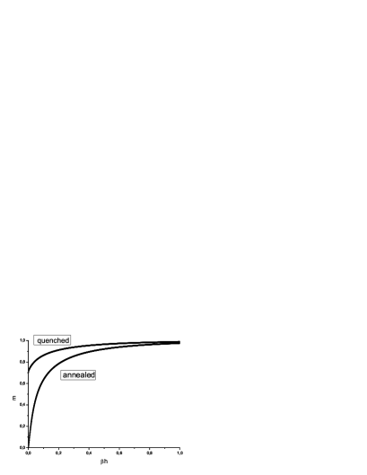
Figure 1: Magnetization curves with $\beta J=0.5$ in presence of topological disorder, where $q_{k}=3,4$ with equal probabilities.

To obtain the magnetization we use the following numerical procedure. At each point $\beta h$, starting from $\beta h=0$ with step $\Delta(\beta h)=0.001$, we get fixed points of the mapping (7). In our simple example, evaluating fixed points one have to replace ${\{x_{k},y_{k}\}}$ and ${\{x_{k-1},y_{k-1}\}}$ in equations (7) on ${\{x,y\}}$. Solution of the obtained system of equations with respect to ${\{x,y\}}$ gets the set of the searched fixed points. In presence of the magnetic field there are only one fixed point holding conditions $x_{k}>0$ and $y_{k}>0$. In case of the zero magnetic field one have two stable fixed points and one nonstable, or otherwise, depending on temperature. For checking stability of the fixed points of (7), one can calculate Jacobian of (7) as

$$J=\left|\begin{array}[]{ll}e^{J+h}x+\frac{3}{2}e^{J+h}x^{2}&e^{-J-h}y+\frac{3}{2}e^{-J-h}y^{2}\\ e^{-J+h}x+\frac{3}{2}e^{-J+h}x^{2}&e^{J-h}y+\frac{3}{2}e^{J-h}y^{2}\end{array}\right|.$$ (10)

The condition of stability now sounds as $|J|<1$.

It is known that the Ising model on Bethe lattice with constant $q$ has a critical point defined by condition $\beta_{c}J=\frac{1}{2}\ln\frac{q}{q-2}$ Baxter . According to Baxter , it is possible to write one dimensional mapping for the partition function of the model with fixed $q$. This mapping has three fixed points in zero magnetic field. It is easy to check that the temperature corresponding to the case of the three non stable fixed points defines by the same condition as the critical temperature. When temperature is less then the critical temperature, one obtains two stable fixed points (spontaneous magnetization) and one non stable $x=1$. For the temperature greater then critical one, we get two nonstable and one stable $x=1$ points. This interpretation of known regimes Baxter around the critical point gives a possibility for the numerical investigation in presence of the topological disorder. For the evaluation of critical temperature of our example $q=3,4$ we propose the following numerical procedure. Starting from point $\beta J=0$ and holding $h=0$, with step $\Delta(\beta J)=0.005$, we check stability of obtained fixed points and looking for $\beta J$ at which two stable points become unstable and the third one becomes stable. The obtained result is not an exact value of the critical temperature, but an interval of possible values. The size of this interval depends on the precision $\Delta(\beta J)$. As a result we found $\beta_{c}J=0.725$, which is greater then the corresponding values for the Ising models on Bethe lattice with fixed $q=3$ and $q=4$.

Another interesting choice of topological disorder is $q=2,3$, where $q$ takes corresponding values with probability $P(q)$. Here we consider only uniform probability distribution $P(2)=P(3)=0.5$. The general study is a subject of further research. The coordination number $q=2$ corresponds to the one dimensional Ising model having zero critical temperature. The existence and localization of the critical point in this mix of one-dimensional Ising model and Ising model on Bethe lattice is a subject of special interest. The main idea is an evaluation of the fixed points of corresponding mapping, as it was done above for $q=2,3$. However, during this procedure one obtains no fixed points holding condition $x>0,y>0$. For any positive initial seed of mapping, after some finite number of iterations (after $15-20$ iterations) $x_{k},y_{k}$ become infinitely big. To deal with these big numbers we define new variable $z_{k}=x_{k}/y_{k}$. The mapping (7) may be represented now as

$$z_{k}=\frac{P(3)(e^{\beta J+\beta h}z^{2}_{k-1}+e^{-\beta J-\beta h})+o(n)}{P(3)(e^{-\beta J+\beta h}z^{2}_{k-1}+e^{\beta J-\beta h})+o(n)}.$$ (11)

The infinitesimals $x_{k}/y^{2}_{k},1/y_{k}$ may be neglected and we obtain that the critical temperature is the same as for Ising model on Bethe lattice with constant $q=3$.

IV Quenched topological disorder

In case of partly annealed topological disorder $0<n<1$ we use the following heuristics. Z quantity may be represented as

$$\textbf{Z}=<Z(\{q_{i}\})^{n}>_{dis}=\sum_{\{q_{i}\}}P(\{q_{i}\})[\exp(\beta h)g_{\{q_{i}\}}^{q_{0}}(+)$$

$$+\exp(-\beta h)g_{\{q_{i}\}}^{q_{0}}(-)]^{n},$$ (12)

where $g_{\{q_{i}\}}(s_{0})$ depends on the particular realization of disorder. One may obtain recursion relations from the previous expression as

$$x_{k}=e^{\beta J+\beta h}x^{q_{k}-1}_{k-1}+e^{-\beta J-\beta h}y^{q_{k}-1}_{k-1}$$

$$y_{k}=e^{-\beta J+\beta h}x^{q_{k}-1}_{k-1}+e^{\beta J-\beta h}y^{q_{k}-1}_{k-1},$$ (13)

denoting $x_{k}=g_{\{q_{i}\}}(+)$ and $y_{k}=g_{\{q_{i}\}}(-)$. It is assumed that on the each step of recursion the power $q_{k}$ takes random values with given probability distribution $P(q)$. The main idea is to consider that although the mapping is stochastic in nature, after some huge number of iterations one would obtain an attractor set of possible pairs $(\overline{x},\overline{y})$ with corresponding stationary probability distribution $P(x,y)$. To find the attractor numerically one may study the mappings (13) with fixed non stochastic values of $q_{k}=q$. The fixed points of those mappings should be a part of searching attractor. One may start stochastic iteration (13) from those fixed points and get the set of possible pairs $(\overline{x},\overline{y})$. There is a possibility of a disconnected attractor (and broken ergodicity), therefore the final set should be based on the summation of sets derived from iterations of all possible fixed points. During the iteration process one gets not only an attractor set but also it is possible to evaluate Z. The method of iterations takes a chance to calculate value of $<[\exp(\beta h)x_{k}^{q_{0}}+\exp(-\beta h)y_{k}^{q_{0}}]^{n}>_{dis}$. Although the numerical and approximate nature of such evaluation we suppose a consistent result in the limit of large number of iterations. The magnetization in presence of partly annealed disorder may be written as

$$m_{dis} = \frac{\int DJP(J)m(J)\exp(-\overline{\beta}F(J))}{\int DJP(J)\exp(-\overline{\beta}F(J))}=\frac{\int DJP(J)\frac{\partial Z(J)}{\partial\beta h}(Z(J))^{n-1}}{\int DJP(J)(Z(J))^{n}}$$ (14)

$$= \frac{<[\exp(\beta h)x_{k}^{q_{0}}-\exp(-\beta h)y_{k}^{q_{0}}]\times[\exp(\beta h)x_{k}^{q_{0}}+\exp(-\beta h)y_{k}^{q_{0}}]^{(n-1)}>_{dis}}{<\exp(\beta h)x_{k}^{q_{0}}+\exp(-\beta h)y_{k}^{q_{0}}]^{n}>_{dis}}.$$

However, the analysis of mapping (13) for the simple example where $q_{k}=3,4$ with equal probabilities demonstrates some difficulties. After few steps of iteration the values of $x_{k},y_{k}$ approach to zero or infinity. To overcome it we propose a mathematical trick, which should give correct values of magnetization for $n\rightarrow 0$ and exact magnetization in presence of quenched topological disorder $n=0$. Instead of $x_{k}$ and $y_{k}$ one may consider new variable $z_{k}=x_{k}/y_{k}$ and write a one dimensional mapping

$$z_{k}=\frac{e^{\beta J+\beta h}z^{q_{k}-1}_{k-1}+e^{-\beta J-\beta h}}{e^{-\beta J+\beta h}z^{q_{k}-1}_{k-1}+e^{\beta J-\beta h}}.$$ (15)

The mathematical trick lies in taking out the means over the disorder $y_{k}$ in Eq. (14), like it is possible to do with constant parameter (real number). It is supposed that if $y_{k}$ is infinite quantity or infinitesimal one, than this approach is reliable. The magnetization may be rewritten now as

$$m_{dis}\approx\frac{<[\exp(\beta h)z_{k}^{q_{0}}-\exp(-\beta h)]\times[\exp(\beta h)z_{k}^{q_{0}}+\exp(-\beta h)]^{(n-1)}>_{dis}}{<\exp(\beta h)z_{k}^{q_{0}}+\exp(-\beta h)]^{n}>_{dis}}.$$ (16)

Previous relation Eq. (16) becomes exact in presence of quenched topological disorder as it follows directly from Eq. (14). Using this trick is easy to get magnetization for our example with $q=3,4$. To obtain magnetization we change the values $\beta h$ like it was done for the annealed version of disorder. We start evaluation of important means after $10^{4}$-th iteration and calculating them using the same number of iterations. The result does not change if this value is greater, therefore we suppose that it is stable. The values of $z_{k}$ are distributed around the fixed points of the mappings (15) with fixed values of $q_{k}$. The dependence of magnetization on external field $h$ in presence of quenched topological disorder is given in Fig (1).

Figure 2: Spontaneous magnetization in presence of quenched topological disorder, where $q_{k}=3,4$ with equal probabilities.

To get the position of the critical temperature for our example $q=3,4$ we use the basic knowledge about spontaneous magnetization. The dependence of the spontaneous magnetization on temperature provides an opportunity to single out the critical point. Iteration process and evaluation of the magnetization under the zero magnetic field, as it was described above, give us dependence of the spontaneous magnetization on $\beta J$ (Fig. (2)). The critical temperature lies between the critical temperatures corresponding to the same models on Bethe lattices with constant $q=3$ and $q=4$ coordination numbers.

The same analysis may be done for the quenched topological disorder with $q=2,3$. Our study of the spontaneous magnetization shows that the critical point exists and the critical temperature differs from zero even when the probability of $q=2$ is greater than the probability of $q=3$ ($P(3)=0.01$, $2<\beta_{c}J<3$). It means that the little possibility of branching in one dimensional Ising model (rare branches) lead to the critical behavior with non zero critical temperature in the thermodynamical limit.

As it is easy to see, we mentioned above some propositions which are very general (statements about attractor and other ) and they need to be studied with mathematical rigor. However, this statements are useful and numerical research gives an evidence of their correctness.

V Conclusion

Summarizing written above, we developed an approach to deal with topological disorder for the spin models on hierarchical lattices. Despite its demonstration only on the simple Bethe lattice, a generalization on more complicated models is straightforward. A wide spectra of problems solving within approach of hierarchical models and having well physical description within it may be revisited now in presence of fluctuating coordination number of lattice. A complicated disorder may lead to the nontrivial solutions of the recursive relations Eq. (7). The distributions of the Yang-Lee and Fisher zeros in presence of disorder is also an interesting problem. Speaking about social dynamics we see that the hierarchical models take a possibility to simplify the problem within Ising paradigm without significant loss of verity and developed approach makes it possible to get the major interesting quantities.

VI Acknowledges

Authors are grateful to E. Mamasakhlisov and A. Allahverdyan for discussions . K.S. would like to thank K. Mazmanian for useful remarks. This work was supported by ANSEF grant PS-condmatth-521.

References

- (1) M. Pretti, Phys. Rev. E 74,051803(2006).
- (2) P. D. Gujrati, Phys. Rev. Lett. 74, 809 (1995).
- (3) M.-S. Chen, L. Onsager, J. Bonner, and J. Nagle, J. Chem. Phys. 60, 405 (1974).
- (4) A. Z. Akheyan, N. S. Ananikian, J. Phys. A 29, 4, 721 (1996).
- (5) N. S. Ananikian, A. R. Avakian, N. Sh. Izmailian, Physica A 172, 391 (1991).
- (6) N. S. Ananikian, R. R. Shcherbakov, J. Phys. A 27, L887 (1994).
- (7) J. Vannimenus, Z. Phys. B 43, 141 (1981).
- (8) E. Albayrak and M. Keskin, Eur. Phys. J. B 24, 505 (2001).
- (9) M. Eckstein, M. Kollar, K. Byczuk, and D. Vollhardt, Phys. Rev. B 71, 235119 (2005).
- (10) D. J. Thouless, Phys. Rev. Lett. 56, 1082 (1986).
- (11) J. M. Carlson, J. T. Chayes, L. Chayes, J. P. Sethna, D. J. Thouless, Europhys. Lett. 5 355 (1988).
- (12) T. Morita, Phisica A 98, 566 (1979).
- (13) M. J. de Oliveira, S. R. Salinas, Phys. Rev. B 35, 2005 (1987).
- (14) C. Castellano, S. Fortunato, V. Loreto, physics.soc-ph: arXiv:0710.3256v1.
- (15) V. Dotsenko, Introduction to the Replica Theory of Disordered statistical systems, Cambridge ; New York : Cambridge University Press, 2001.
- (16) A. E. Allahverdyan, Th. M. Nieuwenhuizen, Phys. Rev. E 62, 845(2000); A. E. Allahverdyan, K. G. Petrosyan Europhys. Lett. 75, 6, 908 (2006).
- (17) V. R. Ohanyan, L. N. Ananikyan, N. S. Ananikian, Physica A 377, 501-513 (2007).
- (18) R.G. Ghulghazaryan, N.S. Ananikian. J.Phys. A., 36, 6297 (2003).
- (19) R.G. Ghulghazaryan, N.S. Ananikian, P.M.A.Sloot. Phys. Rev. E, 66, 046110 (2002).
- (20) N.S. Ananikian, R.G. Ghulghazaryan. J. Comp. Methods in Sciences and Engineering, 2, 75. (2002).
- (21) A.E. Alakhverdian., N.S. Ananikian, S.K. Dallakian. Phys.Rev.E, 57, 2452 (1998).
- (22) L. Monroe. Phys. Lett. A, 188, 80 (1994).
- (23) R. J. Baxter, Exactly Solaed Models in Statistical Mechanics (Academic, London, 1982).