Automated Classification of ELODIE Stellar Spectral Library Using Probabilistic Artificial Neural Networks

Abstract

A Probabilistic Neural Network model has been used for automated classification of ELODIE stellar spectral library consisting of about 2000 spectra into 158 known spectro-luminosity classes. The full spectra with 561 flux bins and a PCA reduced set of 57, 26 and 16 components have been used for the training and test sessions. The results shows a spectral type classification accuracy of 3.2 sub-spectral type and luminosity class accuracy of 2.7 for the full spectra and an accuracy of 3.1 and 2.6 respectively with the PCA set. This technique will be useful for future upcoming large data bases and their rapid classification.

1 Introduction

In recent years, Artificial Neural Networks (ANNs) have become very useful tool for classification type applications (in particular the stellar spectral classification) in astronomy. Some of the pioneering efforts of application of ANNs to stellar spectral classifications are:
Gulati et al. (1994a, 1994b), Gulati et al. (1995), Von Hippel et al. (1994), Weaver et al. (1995), Singh et al. (1998, 2003), Gupta et al. (2004),
and several other groups. All these applications have used ANNs in various forms based on supervised methods where, the computer is trained with certain known classes of spectra and then at the post-training stage, the test set of spectra are input to the program for a quick classification. The use of Principal Component Analysis (PCA) greatly reduces the complexity of the training matrix to a manageable dimension. Most of the previous attempts for automatic classification of stellar spectra were done using backpropagation algorithm but in this work probabilistic neural network Specht D. F., (1990) is presented, which offers some advantages over the backpropagation technique like: fast training process, no local minima issues, guaranteed to converge to an optimal classifier as the size of representative training set increases, though it suffers from some disadvantages like large memory and more representative training set requirements.

The section $\S 2$ discusses the input data format; section $\S 3$ outlines the PNN technique; section $\S 4$ discusses the PCA method; section $\S 5$ gives the performance and results and finally the section $\S 6$ gives the conclusions of this study.

2 THE INPUT DATA

The Jacoby et al. (1984) (hereafter referred as JHC library) was used as sample spectra for training of the neural network. This library covers the wavelength range 3510-7427 Å  for various O to M type star which contains 161 spectra of individual stars and 158 spectra were selected from this library as a set of learning patterns to neural networks. The ELODIE.3 stellar library, Prugniel & Soubiran (2001, 2004) was used as a set of testing patterns to neural network for classification. This library covers the wavelength range of 4000 to 6800 Å  and contains 1962 spectra of which 1959 spectra are selected for the classification. The library is given at two resolutions high and medium of which the medium resolution is selected. The spectral resolution of JHC is 4.5 Å  with one flux value per 1.4 Å  and the ELODIE has a resolution of 0.55 Å  with each flux value at 0.2 Å . Both these libraries were brought to a common platform of spectral resolution of 4.5 Å  and sampling fluxes every 5 Å  steps (a total of 561 bins) and a wavelength range of 4000-6800 Å . This was achieved by using appropriate convolution and spline fitting routines. Both the libraries were also normalized to unity to take care of difference in flux calibration process of two libraries.

3 PROBABILISTIC NEURAL NETWORKS

The Probabilistic Neural Network was introduced by Specht D. F., (1990). This technique can be used for the classification problem and estimation of class membership Specht D. F., (1994). This network is a supervised neural network and its development relies on Parzen windows classifier and is the direct continuation of the work of Bayes classifiers Specht D. F., (1990), Parzen E. (1962). The Parzen windows method is a non-parametric procedure that synthesizes an estimation of a probability density function (pdf) by superposition of a number of windows. The PNN learns to approximate the pdf of the training samples.
In first step the distance between input vector and the training input vectors will be evaluated and then a vector will be produced from which the similarity and closeness of the input to training input will be known. In the next stage the summation of these contributions for each class of inputs will take place in order to produce a vector of probabilities as its net output, and then the maximum of these probabilities will be selected

Figure 1: Schematic of a typical Probabilistic Neural Network

and will be available at the output.
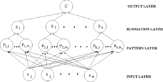
The architecture of a PNN illustrated in Figure 1 with four layers: the input layer, the pattern layer, the summation layer and the output layer. An input vector $X=(x_{1},x_{2},...,x_{n})\in R^{n}$ , is given to the input neurons and then passed to the pattern layer, the neurons of which grouped and each group will be dedicated to one class (or here to one spectra of the training set). The output of the $i^{th}$ pattern neuron of $K^{th}$ group in the pattern layer will be in the form,

$$P_{k,i}(X)=\frac{1}{(2\pi\sigma^{2})^{n/2}}\exp\left(-\frac{\parallel X-X_{k,i}\parallel^{2}}{2\sigma^{2}}\right),$$ (1)

where $X_{K,i}\in R^{n}$ is center of the kernel, $\sigma$ known as the spread or smoothing parameter. Then the summation layer of the network, which computes the approximation of the conditional class probability function given as:

$$S_{k}(X)=\sum_{i=1}^{N_{k}}\omega_{k,i}P_{k,i}(X),\hskip 14.22636ptk\in\{i,....,K\},$$ (2)

where $N_{k}$ is the number of neurons of class k, which in our case $N_{k}$ will be 561. $\omega_{ki}$ are positive coefficients satisfying $\sum_{i=1}^{N_{k}}\omega_{ki}=1$.
Then finally at the output layer we will have:

$$C(X)=arg\max_{1\leq k\leq K}(S_{k}).$$ (3)

As seen in the Figure 1, the pattern layer is fully connected to the input layer, with one neuron for each pattern in the training set. The weight values of the neurons in this layer are set equal to the different training patterns. The summation is carried out by the summation layer neurons. The weights on the connections to the summation layer are fixed at unity so that the summation layer simply adds the outputs from the pattern layer neurons. The output layer neuron produces a binary output value corresponding to the largest pdf, this indicates the best classification for the pattern.

4 PRINCIPAL COMPONENT ANALYSIS

Principal Component Analysis (PCA) is widely used in signal processing, statistics and neural computing. The main idea in using PCA is to extract the components which gives maximum amount of variance. A $1959\times 561$ matrix, which is input data size with 1959 row as the number of spectra to be classified and 561 is the size of each spectra. With the help of PCA first tried to reduce the size of input vectors to simplify the network. The PCA transforms input vector with highly correlated dimension of 561 variables by orthogonal transformation to lower number of uncorrelated variables which are called principal components. The resulting principal components comes in an ordered manner such that the first principal component has the largest variation and it will be in reducing order to the next and subsequent principal components, and it eliminates the variables with lowest variation in the whole spectra.
This technique is applied to both the training and test data sets and the best performance obtained with 26 principal components as shown in the Table 1.

Table 1: Network performance for PNN with PCA and Full Set

Number	Principal Component	r1	s2
1	57	0.924177	452.3178
2	26	0.92483	448.4866
3	16	0.92440	450.2248
4	Full spectra (No PCA)	0.92384	454.6563

1 correlation coefficient, 2 standard deviation

5 PERFORMANCE AND RESULT

5.1 Spectral class coding

The performance of the ANN is judged by a quantitative correlation analysis. The spectro-luminosity classes which are usually in an alpha-numeric fashion, had to be converted into a numeric code number (Gulati et al. 1994a) which is unique to each spectro-luminosity class and is given as follows:

$$CodeNumber=1000.0\times\rm A1+100.0\times\rm A2+(1.5+2\times\rm A3)\\$$ (4)

where A1 represents the spectral type of the star (ranging from O to M which is numbered as 1 to 7); A2 is the sub-spectral type of the star (with codes ranging from 0.0 to 9.5); and A3 is represents the luminosity class of the stars (ranging from I to V classes which is coded into numbers ranging from 0 to 4). For example consider alpha-numeric spectro-luminosity class F3II which will be coded as 4303.5 and K9.5V will be coded as 6959.5.

Table 2: LIST OF SPECTRA APPEARING IN FIGURE 4

Panel	Jacoby	Jacoby	ELODIE	ELODIE
	Spectra	Spectral	Spectra	Spectral
		Class		Class
a	HD 10032	4009.5	HD 338529	2509.5
b	SAO 87716	3301.5	HD 190864	1705.5
c	SAO 87716	3301.5	HD 000108	1609.5
d	HD 23733	3909.5	HD 172488	2059.5
e	TR A14	5409.5	HD 017378	3501.5
f	HD 26514	5605.5	HD 216131	7205.5
g	HD 12842	4301.5	HD 049330	2009.5
h	SAO 21536	4401.5	HD 172488	2059.5
i	BD $58\,^{\circ}$ 0204	4201.5	HD 225160	1809.5
j	BD $00\,^{\circ}$ 3227	4503.5	HD 172488	2059.5
k	SAO 21536	4401.5	HD 018409	1901.5
l	SAO 21536	4401.5	HD 192639	1809.5
m	HD 56030	4605.5	HD 016429	1955.5
n	SAO 21536	4401.5	HD 015558	1509.5
o	SAO 21536	4401.5	HD 015629	1509.5
p	HD 107399	4909.5	HD 184499	1009.5

5.2 Performance

The performance of the classification is evaluated by correlation analysis. The list of 1959 ELODIE.3 spectra classified by different networks with different number of principal components was correlated with respect to the catalog classification given in ELODIE at the web site:

http://www-obs.univ-lyon1.fr/$\sim$prugniel/soubiran/v3/table_meas.dat

Table 1 shows the network performance estimated from the linear correlation coefficient, r, and the standard deviation, s, of the network and catalog classification. The best performance is for the network with 26 Principal Components (PCs) with lowest standard deviation and largest correlation coefficient.

Table 3: LIST OF SPECTRA REJECTED IN PNN WITH PCA

Spectra	Catalog	ANN Class	Error
Name	Class
HD002796	4109.5	5309.5	-1200
HD014374	5009.5	6009.5	-1000
HD014626	6009.5	7009.5	-1000
HD017925	6109.5	5001.5	1108
HD019445	3409.5	4509.5	-1100
HD034078	1959.5	3301.5	-1342
HD034078	1959.5	3301.5	-1342
HD038237	3309.5	4601.5	-1292
HD043823	4209.5	5409.5	-1200
HD045674	4009.5	5409.5	-1400
HD048279	1809.5	2805.5	-996
HD099649	5509.5	4009.5	1500
HD099649	5509.5	4009.5	1500
HD154543	6209.5	7305.5	-1096
HD163346	3309.5	4503.5	-1194
HD184499	1009.5	4909.5	-3900
HD205811	4209.5	3109.5	1100
HD216131	7205.5	5301.5	1904
HD218502	4309.5	2101.5	2208
HD338529	2509.5	4009.5	-1500
HD039681	2909.5	3909.5	-1000
BD+362165	5009.5	4007.5	1002
HD000108	1609.5	2701.5	-1092
HD000108	1609.5	3301.5	-1692
HD001835	5309.5	7303.5	-1994
HD008992	4601.5	5909.5	-1308
HD013267	2501.5	4201.5	-1700
HD013268	1809.5	2801.5	-992
HD014947	1609.5	3909.5	-2300
HD015558	1509.5	4401.5	-2892
HD015570	1409.5	4605.5	-3196
HD015629	1509.5	4401.5	-2892
HD016429	1955.5	4605.5	-2650
HD016429	1955.5	4605.5	-2650
HD016429	1955.5	4605.5	-2650
HD017145	2801.5	5309.5	-2508
HD017378	3501.5	5409.5	-1908
HD018409	1901.5	4401.5	-2500
HD024496	5009.5	6009.5	-1000
HD034078	1959.5	3301.5	-1342

Table 4: Table 3(Contd.)

Spectra	Catalog	ANN Class	Error
Name	Class
HD034078	1959.5	3301.5	-1342
HD049330	2009.5	4301.5	-2292
HD053003	5001.5	6009.5	-1008
HD054908	3009.5	4009.5	-1000
HD057838	6209.5	5101.5	1108
HD089010	5207.5	7509.5	-2302
HD096094	5009.5	3805.5	1204
HD110184	5509.5	6705.5	-1196
HD157857	1709.5	2701.5	-992
HD159307	4809.5	3809.5	1000
HD161370	3009.5	4009.5	-1000
HD166734	1809.5	5001.5	-3192
HD170739	2809.5	4009.5	-1200
HD172171	6105.5	7505.5	-1400
HD172488	2059.5	3909.5	-1850
HD172488	2059.5	4401.5	-2342
HD172488	2059.5	4503.5	-2444
HD174512	2809.5	4503.5	-1694
HD178359	4507.5	5803.5	-1296
HD182736	5009.5	6009.5	-1000
HD182736	5009.5	6009.5	-1000
HD186980	1759.5	2801.5	-1042
HD190864	1705.5	3301.5	-1596
HD192639	1809.5	4401.5	-2592
HD195592	1951.5	4809.5	-2858
HD199579	1609.5	2701.5	-1092
HD202124	1951.5	4301.5	-2350
HD206165	2201.5	3301.5	-1100
HD210839	1609.5	3301.5	-1692
HD213470	3301.5	4309.5	-1008
HD216131	7205.5	5605.5	1600
HD216572	3009.5	4709.5	-1700
HD217086	1709.5	4605.5	-2896
HD223385	3301.5	4709.5	-1408
HD225160	1809.5	3301.5	-1492
HD225160	1809.5	4201.5	-2392

Figure 2: ELODIE library classification using PNN with PCA before rejection

Figure 3: ELODIE library classification using PNN with PCA before rejection

Figure 4: Plots of Jacoby library vs. ELODIE library listed in table 2.

Figure 5: 3-D Scatter diagram of ELODIE library classification using PNN with PCA after rejection

5.3 Result

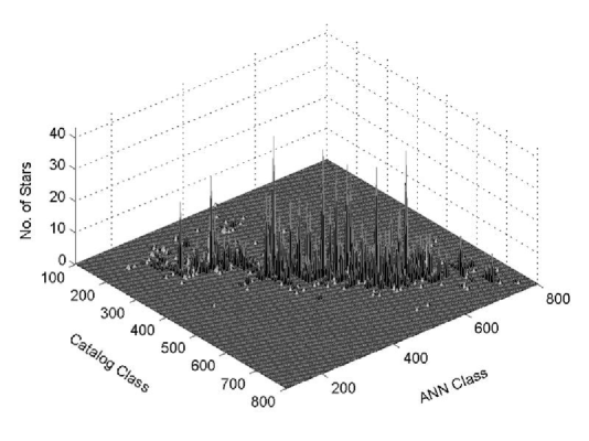
The Neural Network with PNN technique is used to obtain the results given in Table 1. The result of the classification is in the form, such that, for each spectra of ELODIE library (test set for ANN), there is a corresponding spectra from JHC library (training set for ANN) which is its respective spectro-luminosity class. This result is given in Table 7 where the name of the star, their spectral and luminosity class given by ANN and Catalog (the web site given at $\S 5.2$) are presented. The result of the classification of PNN with 26 PCs is presented in a 3D scatter plot format in Figure 2. This figure also shows the number of spectra available at each spectral type and luminosity class.

Figure 3 is another 3D picture of classification errors in spectral type and luminosity class shown on the horizontal axis. Some of the misclassified spectra with large classification errors are presented in Figure 4 where, 16 panel shows 16 misclassifications according to the ANN result. The spectra in dotted lines represent those from the learning library (JHC) and the spectra in solid lines are the corresponding ones from the test library (ELODIE). Table 2 describes the details of Figure 4 with the names of the spectra plotted in each panel and their coded spectral class. These plots contribute to the largest classification errors (i.e. high difference between ELODIE class in Catalog and class obtained by ANN). But the plots does not support this and shows good match of these pairs of spectra. So, the classes obtained by ANN could be the correct class of those spectra.

The result of ANN produced in two schemes:

(1) With PCA:

In this scheme first, PCA reduction technique is applied to reduce the size of spectra from 561 to 26 PCs and then PNN is used for automatic classification. As seen from the scatter plot in Figure 2, there are some spectra which are outliers and contribute to the large errors in the classification result; these spectra are rejected and their list is given in Table 3. This table gives the name of rejected spectra, their class given by catalog and that of obtained from ANN and the corresponding error.

The accuracy of the classification is evaluated separately for the Spectral Type (ST) and Luminosity Class (LC) before and after rejection of the spectra listed in Table 3 from the result of classification of PNN with PCA, and the summary of this is given in Table 4.

Table 5: ACCURACY OF CLASSIFICATION FOR PNN WITH PCA

Accuracy before rejection	Accuracy after rejection
4.4 ST	3.1 ST
2.7 LC	2.6 LC

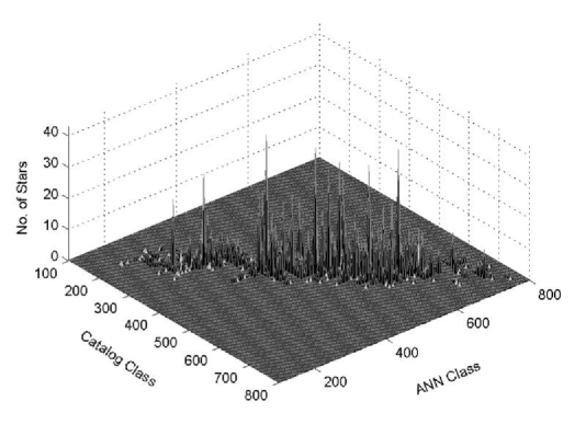
After rejecting the spectra listed in Table 3, the 3D scatter plot is shown in Figure 5.

(2) Without PCA:

In this scheme the PNN is applied to whole spectra of size 561 flux bins. The list of spectra rejected in this scheme is same as in the Table 3, in addition with the spectra listed in Table 5.

Table 6: LIST OF REJECTED SPECTRA FOR PNN WITHOUT PCA

Spectra	Catalog	ANN Class	Error
Name	Class
HD016429	1955.5	4309.5	-2354
HD110184	5509.5	6603.5	-1094
HD166734	1809.5	5101.5	-3292
HD172488	2059.5	4307.5	-2248
HD199579	1609.5	3001.5	-1392
HD216131	7205.5	5705.5	1500

The accuracy of the classification for ST and LC before and after rejection given in the Table 6.

Table 7: ACCURACY OF CLASSIFICATION FOR PNN WITHOUT PCA

Accuracy before rejection	Accuracy after rejection
4.5 ST	3.2 ST
2.8 LC	2.7 LC

6 CONCLUSION

The classification of ELODIE on the basis of JHC, then comparing the result of ANN classification with catalog classes and scanning for the spectra contributing to higher error and plotting them, shows that though the spectral class given in catalog is different than that of given by ANN for these plots, but Figure 4 show that they are of same spectro-luminosity class and it supports ANN classification result. So by considering these corrections for misclassification the standard deviation values given in Table 1 will be much lower and also the classification accuracy will improve. The whole set of ELODIE library is classified with JHC library as reference to the spectral type accuracy of 3.2 sub spectral type and luminosity class accuracy of 2.7 for full spectra and spectral type accuracy of 3.1 sub spectral types and luminosity class accuracy of 2.6 for PNN with 26 PCs.

The classification of all of the ELODIE test spectra was done in few seconds, so classification of very large spectral libraries can be done in considerably short time using this technique in future.

References

- [1] Gulati, R. K.; Gupta, R.; Khobragade, S. 1994a, ApJ, 426, 340.
- [2] Gulati, R. K.; Gupta, R.; Khobragade, S. 1994b, Vistas in Astronomy, 38, 293.
- [3] Gulati, R. K.; Gupta, R.; Khobragade, S. 1995, Astronomica Data Analysis Software and Systems IV, ASP Conference Series, 77, R. A. Shaw, H.E. Payne,and J.J.E. Hayes, eds. p.253
- [4] Gupta, Ranjan; Singh, Harinder P.; Volk, K.; Kwok, S. 2004, ApJS, 152 Issues 2, 201.
- [5] Jacoby, G. H.; Hunter, D. A.; Christian, C. A. 1984, ApJS, 56, 257.
- [6] Parzen E. 1962, Annals of Mathematical Statistics, 3, 1065.
- [7] Prugniel Philippe, Caroline Soubiran. 2001, A&A, 369, 1048.
- [8] Prugniel Philippe, Caroline Soubiran. 2004, astro-ph/0409214 v2.
- [9] Singh, Harinder P.; Gulati, Ravi K.; Gupta, Ranjan. 1998, MNRAS, 295, 312.
- [10] Singh, Harinder P.; Gupta, Ranjan. 2003, Large Telescopes and Virtual Observatory: Visions for the Future, 25th meeting of the IAU, Joint Discussion 8.
- [11] Specht D. F., 1990, Neural Networks, 1(3), 109.
- [12] Specht D. F.; H. Romsdahl. 1994, In Proceedings of the IEEE International Conference on Neural Networks, 2, 1203.
- [13] Von Hipple, T.; Storrie-Lombardi,L. J.; Storrie-Lombardi,M. C.; Irwin,M. J. 1994, MNRAS, 269, 97.
- [14] Weaver, Wm. Bruce; Torres-Dodgen, Ana V. 1995, ApJ, 446, 300.